Crystal Structure Refinement

Transcription

1 Crystal Structure Refinement Dr. Falak Sher Pakistan Institute of Engineering and Applied Sciences Islamabad 09/10/2010

2

3 The Rietveld Method Rietveld structure refinement is a method for estimating the intensities of Bragg peaks in a powder diffraction pattern within the constraints imposed by a crystallographic space group. The entire diffraction profile is calculated (model) and compared with the observed profile point by point A trial structure (model) is used to calculate the intensities of the peaks in the experimental pattern The parameters of the model are then adjusted using the Least-Square method to obtain the best fit The Model (3 parts) 1. Crystallographic Model: describes size, symmetry of unit cell, atomic positions, thermal parameters and occupancy 2. Instrumental Model: describes optics and set-up of diffractometer 3. Profile Model: describes peak shape Model data is minimised iteratively until satisfactory answer, i.e. a good fit between experimental and calculated pattern is obtained.

4 Mathematical Basis Rietveld refinement is based on the least-squares minimization of the residual S = w y where w i is a suitable weight, given by i i io y ic 2 σ ip is the standard deviation associated with the peak and σ ib is that associated with the background intensity, y ib ; y io is the intensity observed at the ith step, y ic is the sum of contributions from neighbouring Bragg reflections and from the background calculated according to ic ( ) w = σ = σ + σ i k k i k k ( ik ) yib y = s m L F G θ + where s is a scale factor, m k is the multiplicity factor, L k is the Lorentz polarization coefficient for the reflection k, F k is the structure factor, G is the reflection profile function, θ ik = 2θ i 2θ k, 2θ k is the calculated position of the Bragg peak and y ib is the background intensity. Ideally S = 0 2 ip ib

5 Parameters not included in the above equation are: Structural Parameters: Unit cell parameters: (a,b,c;α,β,γ): they can be refined but are not included in the equation and should be close to real cell parameters. Space Group: cannot be refined. Must be right

6 Peak Shape Function

7

8 The agreement between the observations and the model is estimated by the following indicators: The profile R p R p = yio yic /( yio ) The weighted profile R wp R w ( y y ) [ ] 2 2 / w y 1/ 2 wp = i io ic i io The Bragg R B R B = I ko I kc /( I ko ) The values of I ko are obtained by partitioning the raw data in accordance with the I kc values of the component peaks. The expected R E 2 R [( N P) ( w y )] 1/ 2 E = i io Goodness of fit or the reduced χ 2 / 2 χ 2 ( y y ) ( N P) = w / i io ic where N is the total number of observations in all histograms and P is the number of variables in the least squares refinement. It should reach the ideal value of unity.

9

10 Where to get crystal structure information check if the structure is already solved websites Inorganic Crystal Structure Database (ICSD) 4% is available for free online as a demo Crystallography Open Database Mincryst American Mineralogist WebMineral databases PDF4 from the ICDD Linus Pauling File from ASM International Cambridge Structure Database literature use the PDF to search ICSD listings and follow the references look for similar, hopefully isostructural, materials index the cell, and then try direct methods or ab-initio solutions beyond the scope

11 Free GSAS + ExpGUI Fullprof Rietica PSSP (polymers) Maud (not very good) Rietveld Programs PowderCell (mostly for calculating patterns and transforming crystal structures, limited refinement) Commercial PANalytical HighScore Plus Bruker TOPAS (also an academic) MDI Jade or Ruby

12 Ray Young s Refinement Strategy Scale factor Zero shift Linear background Lattice parameters More background Peak width, w Atom positions Preferred orientation Isotropic temperature factor B U, V, and other profile parameters Anisotropic temperature factors

13 Rietveld Refinement of Powder Diffraction Data by using GSAS/EXPGUI This exercise provides a tutorial example of how to use the GSAS software package with the EXPGUI interface to perform Rietveld analysis. X-ray diffraction data file (GSAS format) of corundum (alumina, Al 2 O 3 ), instrument parameter file and starting cell parameters and atomic positions are provided. Rietveld analysis works using non-linear least-squares fitting to optimize (refine) parameters. This means that we must start with approximate values for all parameters that will be fit. We then allow the software to optimize a small subset of the parameters a minimal number of parameters that must be fit before any progress can be made. Slowly, additional parameters are selected to be refined, until all parameters in the model (if the data support that) are refined. Despite the simplicity of the material, this exercise demonstrates many of the procedures needed for more complex materials.

14 Getting Started To perform this tutorial on your own computer, you will need to have GSAS and EXPGUI downloaded on your computer. These softwares are freely available from the website: You will also need following three files: 1. Raw data file (GSAS format) 2. The instrument parameter file 3. Unit cell and atomic coordinates information Tutorial Outline 1. Create a GSAS Experiment File 2. Adding a phase 3. Specifying Powder Diffraction Data (Adding a Histogram) 4. Changing the Background Function 5. Initial Fitting: Refine Scale Factor and Background 6. Plotting the Initial Fit 7. Fitting the Unit Cell

15 8. Fitting the Diffractometer Zero Correction 9. Initial Fitting of Profile Parameters 10. Group U iso parameters & Refine coordinates and Overall U iso 11. Finishing Up Sample files 1. al2o3.gsa the alumina neutron diffraction data 2. btdemo.ins the instrument parameter file 3. Alumina_Cell-Parameters.doc a word file with unit cell and atomic parameters 1. Creating an Experiment File In this exercise we will use the EXPGUI interface to access the features of GSAS. On windows, EXPGUI is started by clicking on the appropriate desktop icon. After starting the EXPGUI, a GSAS Experimental (.EXP) file must be selected. The.EXP file is the heart of a GSAS refinement. While other files are used by GSAS programs, all structural information and control parameters are contained within this file.

16 The window shown to the right is opened when EXPGUI is started, where.exp file to be used is selected. The first step in this tutorial is to select the directory where the al2o3.gsa and btdemo.ins files were placed. Do this by clicking on the "Directory" button at the top of the window, or by navigating up and down the directory tree by clicking on the "<Parent>" or individual directory names. Once the correct directory has been selected, the next step is to create a new, empty,.exp file. To do this, the file name we wish to use (corundum) is typed into the bottom box of the file selection window. Note that the capitalization you use here does not matter and.exp is added by default. After the name has been entered press the "Read" button or press the keyboard "Enter" key. To make sure that you really intend to create a new Experiment file, rather than the more common task of opening a previous file, the warning message to the right is displayed and you must click on the "Create" button to continue.

17 At this point, you are prompted to provide an overall title for the experiment file. Enter anything you would like (preferably something that will remind you what you were doing a year from now, when you try to figure out what this strange file was for). When you have finished entering information, press the "Set" button. At this point, the Experiment file, CORUNDUM.EXP, has been created and EXPGUI displays what (little) information can be found in this file. Note that the title is displayed near the top of the window in a "edit" box -- this title can be changed simply by typing into the box. Above the title is the last "history record." GSAS records a history record each time a program is run that modifies the.exp file and this information is displayed here. In the next step we will start adding information to this experiment file.

18 2. Adding a Phase When a GSAS experiment file is first created, a fair amount of information must be supplied before the refinement of parameters can be started. At a minimum, a crystallographic phase must be defined, a set of diffraction data must be loaded and a starting values for experimental parameters must be defined. Fortunately, this can be a fairly simple operation with GSAS and EXPGUI. In this part we will show how a crystallographic phase is specified in EXPGUI. For a mixture, this step would be repeated for each crystallographic phase. If an impurity is identified in a later stage of the refinement, this step can be run at that point to define this additional crystallographic phase. GSAS allows up to nine crystallographic phases to be included in a model. To enter information about a crystallographic phase, modify crystallographic parameters, or select crystallographic parameters to be optimized, the "Phase" panel must be selected by clicking on the "Phase" tab in the upper left of the EXPGUI window. The window then appears as shown on the next page.

19 The next step is to press the "Add Phase" button in the upper left. The "Add New Phase" window, shown below is then generated.

20 Information about the phase can be added directly into the boxes, or phase information can be read from a Crystallographic Information File (CIF). After entering the cell parameters Add button is pressed. One of the places where errors occur in the preparation of GSAS input is in the entering of space group symbols. For this reason, after the Add" button is pressed, a window such as the one below, is created to help you confirm that the correct space group has been entered.

21 It is recommended that you read through this information to check that this is correct. As an example of a possible error, if one entered the corundum example in the rhombohedral setting, rather than the hexagonal setting, then the space group should be entered as "R -3 c R" (where the final R indicates the rhombohedral setting). The listing of lattice centering vectors is only appropriate for the hexagonal (centered) cell. Since the symmetry information is correct in this example, press the "Continue" button on the "check symmetry" window. Now we need to enter atom coordinates for this phase. Press Add New Atoms Enter atom type and coordinates of Al and O in appropriate boxes. These values are given in the word file provided. More atom boxes can be created if required by pressing More Atom Boxes. After entering atom coordinates for both Al and O, press Add Atoms at the lower left to continue.

22 After pressing the "Add Atoms" button, the two atoms are added to the experiment and the phase panel appears, as below.

23 3. Specifying Powder Diffraction Data (Adding a Histogram) GSAS uses the term "histogram" to refer to a diffraction data set. GSAS can fit a model to up to 99 histograms simultaneously, although the majority of refinements done in GSAS use a single histogram or at the most only a few histograms. GSAS can use single crystal or powder diffraction data, either neutron or x-ray. For neutron powder diffraction data, the data can be obtained from either time-of-flight (TOF) or constant wavelength (CW) instruments. GSAS can use x-ray data from synchrotron, laboratory alpha-1,2, and even energy-dispersive x-ray instruments. Two files are needed to load a powder diffraction histogram. The first is a file containing the powder diffraction data, often called a GSAS raw data file (often using the extension.raw,.gsa or.gsas) and the second file is an instrument parameter file (.INS or.inst) that defines what type of data is included in the raw file (x-ray/neutron, CW/TOF/ED, etc.) as well as starting values for the diffractometer constants and peak shape parameters. There are a number of available formats for the raw data files and types of records in the instrument parameter file; this information is defined in the GSAS documentation. Note that raw data files can contain more than one set of data and that an instrument parameter file can contain more than one set of parameters. This feature is rarely used, with the exception of TOF instrumentation, where detectors are grouped into banks and the results for each bank are included in a single file. Software for translating diffraction data into a format accepted by GSAS is available at most user facilities or can be found at the web site. Appropriate instrument parameter files can usually be provided by the instrument scientist at a user facility or prototypes can be found in the GSAS distribution files.

24 This part of the tutorial demonstrates how the alumina powder diffraction data are now added to the experiment file. The Histogram panel is selected by clicking on the Histogram tab, as is shown below. In this case, no data has been defined, as can be determined by the absence of entries in the histogram selection box, in the upper left. The "Add New Histogram" button, at the lower right, is used to add [additional] powder diffraction data sets to the refinement, as will be demonstrated in this page. The histogram panel is used to modify various parameters associated with each set of diffraction data, for example the diffractometer constants (such as wavelength), the background function and terms.

25 Press the "Add New Histogram, the window shown to the right will be displayed. The entries on this window are usually considered from top to bottom. The "Dummy Histogram" option is used to simulate powder diffraction data, and is not used in this tutorial example. So the next item of interest is to select a data file. This is done by pressing the upper of the two "Select File" buttons. Pressing the "Select File" button creates a file open window. Select the input file for this exercise, al2o3.gsa. Double-click on the entry, or select is and press the "Open" button. This open window will then close. Similarly select and enter the instrument parameter file, btdemo.ins, The "Usable data limit" sets the maximum range of data to be used in fitting. This is usually determined by plotting the data to see where no further peaks are present. This can be done here with the GSAS RAWPLOT program. For this exercise, change the default value (the entire data range) to 155 degrees, to exclude a single very broad high-angle peak. The press the "Add button in the lower left.

26 After the "Add" button is pressed, the EXPGUI program runs a GSAS program, EXPTOOL, that actually adds the data reference to the experiment. If an error occurs, its result is shown. If no error occurs, the histogram panel is redisplayed, but this time a histogram appears in the upper left, as seen below.

27 4. Changing the Background Function GSAS offers approximately 10 different background functions (not all are implemented in EXPGUI). For each of these functions, the number of terms to be used is adjustable. The more terms the more complex the shape that can be fit. Each of these background functions has different shapes, and in theory, each function will have advantages under different circumstances. However, we find that the Shifted Chebyschev (type #1) is preferable to the others for the vast majority of Rietveld refinements and almost never used any other function. When a histogram is first added in GSAS, the background function is set to the Cosine Fourier series option (type #2) with two adjustable terms. In this section of the tutorial, we will change the background function and the number of terms. Note the "Refine background" check box has been selected -- this means that the background parameters will be refined (optimized) when GENLES is run. The damping parameter to the immediate left is set to 0 -- this means that the full computed shift will be applied. In cases where a refinement has trouble reaching a minimum, it may be advantageous to increase damping (a setting of 1 implies 90% of the computed shift will be applied and a damping setting of 9 yields a shift of 10%.) Every refinable parameter in GSAS has a refinement flag (either for the group, as in this case, or for each individual parameter) and a damping parameter.

28 To change the background function, press the "Edit Background" button on the histogram panel. After the "Edit Background" button is pressed, the "Edit Background" window opens. In this window both the function type and the number of terms can be changed. Clicking on the "Function type" menu offers a choice of function types. Choose function type #1, the Shifted Chebyschev function. Also in the "Edit Background" window, press on the "Number of terms" button and change this number to 6. Note that with the Chebyschev polynomial arbitrary (including zero) starting values for the background terms is acceptable. After the "Set" button is pressed, the changes are then seen on the histogram panel, as shown on next page. Note that by default, the refine background flag is set, allowing these parameters to be optimized.

29

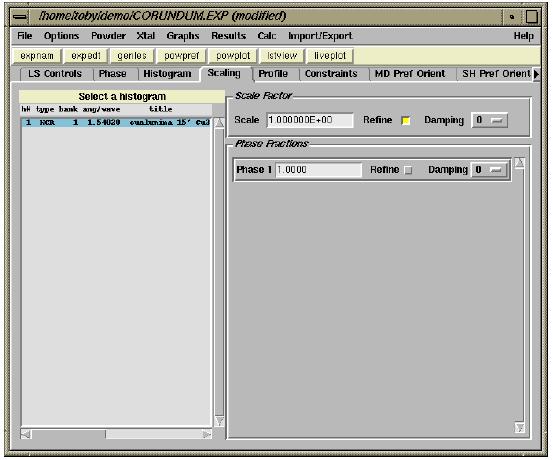
30 5. Initial Fitting: Refine Scale Factor and Background At this point we are almost ready to start fitting parameters, but before we do that the POWPREF program must be run. In GSAS, each data point has a list of reflections that contribute to that data point. This assignment must be made in POWPREF before the least squares fit can be performed in the GSAS program GENLES. The program must also be rerun if a new phase or histogram is added to the refinement. POWPREF should also be rerun if the lattice constants or profile terms change significantly. We want to refine the background and the scale factor to get started. The scaling parameters are shown on the Scaling panel, shown next page. GSAS offers us an overall scale factor for each histogram, plus a phase fraction scale factor for each phase. These two factors have exactly the same effect for a single-phase refinement, so only one can be used. By default, the scale factor refinement flag is turned on and the phase fraction is off. This is what we will use.

31

32 The other change that we will make in the default refinement options is to lower the number of refinement cycles to 2. Also, make sure the "Extract F obs " check box on the least-squares pane is selected.

33 We are now ready to start running programs. First run POWPREF by pressing the POWPREF button on the tool bar. That causes a window, such as the one below to open as POWPREF runs. When POWPREF has completed, press the ENTER key to continue and the window should close. The POWPREF program makes changes to the experiment (.EXP) file and this is noted by EXPGUI by the display of the warning message to the right. At this point you do want to accept the changes made by POWPREF, so click "Load New" and EXPGUI will reread the revised file.

34 By default, this window is shown every time the experiment file is modified by any GSAS program. This allows the file to be "rolled back" to the previous version, in case of a disastrous refinement run, by pressing "Continue with old." However, some EXPGUI users find it annoying to be asked this question all the time. In the EXPGUI Options menu, there is a menu item called "Autoload EXP". If the "Autoload EXP" option is checked, the experiment file will always be read automatically, but then it is no longer possible to roll back erroneous steps so easily. Note that the displayed history record has been updated to reflect the running of POWPREF.

35 We can now initiate the refinement, by launching the GENLES program to optimize the scale factor and background parameters. The output from this run is shown below. After the refinement completes, press Enter to continue and then press "Load new" on the "Reload?" window.

36 The output from the GENLES run shows several points worth noting. First note that the number of variables (varied parameters) is 7, from the scale factor plus the 6 background terms. Note that the initial weighted R-factor (w Rp or R wp ) and Chi-squared values are 99% and 258, respectively but drop to 72% and 134, respectively after a cycle of refinement. In the first cycle of refinement, there are very large shifts in the parameters, but the parameters converge in the second cycle. This is noted by the sum[(shift/esd)**2] term which is 855 in the first cycle, but 0 in the second cycle. Note that shifts become insignificant when they are small with respect to the esd (standard uncertainty), so a value of 855 means that at least some of the parameters made very large shifts in the first cycle. Note that GSAS does not compute the R-factor or Chi-squared terms after the second refinement cycle. 6. Plotting the Initial Fit While Chi-squared and R-values provide some measure of how a fit is progressing, the only way to actually understand the quality of the fit and what problems need to be corrected, is to look at agreement between the observed diffraction data and the corresponding values computed from the fit. This is sometimes called a Rietveld plot. The GSAS program POWPLOT and the EXPGUI program LIVEPLOT allow the fit to be examined graphically. In this tutorial step, LIVEPLOT is used to examine the results.

37 Press the LIVEPLOT button on the button bar (or use a menu command) to start LIVEPLOT. You should then see a plot like the one below. In this plot, the data are "X" characters, the calculated values are a red line. The fitted background is shown as a green line. Offset below, the observed pattern minus the computed pattern is shown in blue. The observed and computed values do not agree very well, but seem to follow the same trends. In the subsequent plots we will see in more detail what some of the discrepancies are. Note that the size of the plot can be changed by changing the size of the window.

38 It will help to see the actual positions of the reflections. This display can be turned on by pressing the "1" key (1 for phase 1, 2 for phase 2...) in the LIVEPLOT window. (This can also be done using the Tickmarks submenu in the File menu.) Note that the color, length, style, placement of the tick mark lines can be changed in the Options menu. Note also that the reflection indices for a tick mark can be displayed by pressing the "h" key when the cursor is positioned over a tick mark.

39 With all the data displayed, it appears that the tick marks are in the right places at lower angles, but are not well placed at 140 degrees and higher. It would be good to see the plot at high magnification to see more detail, however. "Zooming in" is accomplished by clicking the mouse in the lower left and upper right corners of the region to be viewed (lower right & upper left also works). A box is displayed, as below, after the first mouse click. After the second the plot is redrawn.

40 Note with the plot zoomed in, it can now be seen that the lattice parameters do not index the peak 42 degrees very well. The computed peak widths agree reasonably well with the observed.

41 The fit is even worse at high angle. Also, the computed peak widths are much narrower than the observed.

42 Frequent users of LIVEPLOT & BKGEDIT will find that many useful actions can be performed very easily by learning the following keystroke commands. Note that either uppercase or lowercase letters may be used. H A D Z Labels reflections near cursor Labels all reflections Deletes reflection labels Specify zoom range manually 1, 2,... Displays reflection positions (tickmarks) for histogram 1, 2 etc. N L Loads next histogram Turns on display of cursor position arrow keys Moves zoom region around in plot

43 7. Fitting the Unit Cell In the previous tutorial, we saw that the unit cell was not doing a very good job of indexing the diffraction peaks. Since a large number of peaks did have computed reflections at least partly overlapping the observed peaks, we are close enough to fit the unit cell parameters using a refinement. If that were not true -- the tick marks did not fall in the range of the peaks, refinement would not be possible. On the Phase panel, turn on the flag to refine the unit cell parameters (upper right), as shown below.

44 Also, increase the number of cycles to 6 on LS Controls. Run GENLES (as before). Note there are now 9 parameters (scale, 6 background, + 2 cell) and that the fit significantly improves, as seen below. As before, press Enter & load the modified experiment file into EXPGUI.

45 The peak positions are fit much better than before, as seen in the LIVEPLOT output below. Since the peak positions have changed significantly, we now need to rerun POWPREF and use the new peak positions to decide which data points need to be indexed with each reflection.

46 It is not strictly necessary to run GENLES again, but note that CHI-squared improves from 70 to 60 just from the better indexing.

47 8. Fitting the Diffractometer Zero Correction Now that the unit cell parameters have been fit, it is now a good idea to also refine the diffractometer zero correction. The diffractometer zero correction refinement flag is found on the histogram panel, as seen below. Click on the check box for the zero correction near the middle of the window to refine the parameter.

48 Note that the diffractometer zero correction is refined for parallel beam instruments, such as neutron and synchrotron diffractometers. It should not be used for Bragg-Brentano instruments (laboratory flat-plate parafocussing instruments). For Bragg-Brentano instruments, instead the sample displacement parameter (shft) should be refined instead. When needed, for Bragg-Brentano instruments, the sample transparency correction (trns) may also be refined. When GENLES is run, as shown below, a small but significant improvement is seen in the agreement factors.

49 Note that the zero correction has refined from the starting value of 0.04 ( degrees two-theta) to 1.73 ( degrees two-theta). This small correction is needed to obtain a good fit and accurate lattice parameters.

50 9. Initial Fitting of Profile Parameters After the unit cell is fit, the next step is typically to improve the crystallographic model if the profile is well-fit. In this case, however, we cannot do that since the high-angle peaks are much broader than the calculated pattern. This is demonstrated clearly in the LIVEPLOT output shown below. The plot shows several problems that need to be addressed by refining parameters. As noted before, the observed peaks are significantly broader than the calculated, this is addressed by optimizing the peak shape parameters. Also, the relative intensities in the calculated pattern does not match the observed intensities, this can potentially be addressed by refinement of coordinates and, to a lesser extent, individual displacement (temperature) parameters. It is also worth noting that the computed background is too high at higher two-theta values. This may be improved by refinement of the background when the peak intensities are better fit or may require the addition of more background parameters. In any case, neither the coordinates or the background can be effectively optimized until a reasonable fit is obtained for the peak shape.

51 In the Profile panel shown below, the three Gaussian peak width terms (GU, GV & GW, also known as the Cagilloti terms U, V & W), are added to the refinement. After the flags are set for the profile terms, the GENLES program is rerun. At this point, the fit improves considerably.

52 If the fit is examined closely at this stage with LIVEPLOT (as shown below), it can be seen that the peaks at high angle appear to be truncated on each side. This is due to the fact that the peak profiles have gotten much broader, but POWPREF has not yet been rerun, so not enough data points are included in the computation. This sort of problem occurs fairly commonly for neophyte GSAS users. The way to avoid this is to remember to rerun POWPREF after any significant change in the lattice parameters, zero correction or peak profile terms. Also be sure to run POWPREF after adding phases, histograms or changing the excluded regions.

53 Run POWPREF and then GENLES again. Note that still more improvement is seen in the Chi-squared and R-factors. Now LIVEPLOT shows a normally-shaped diffraction peak.

54 10. Refine Coordinates and Overall U iso At this stage in the refinement we have a good fit for the experimental parameters, but need to improve the crystallographic model. To reduce the number of parameters needed in the initial stages of this part of the process, we will define a constraint that requires a single overall U iso value for all atoms. Note that at this stage in the refinement, the peak shape agrees well, but there are significant differences between the observed and computed intensities. This implies that the crystallographic model is in some way inadequate.

55 To group atoms so that they share a single atomic displacement parameter (displacement parameter is the preferred name for "temperature factor"), the parameters need to be constrained together. The Constraints panel allows constraints to be defined to link parameters together. At present EXPGUI allows constraints to be created for atomic parameters and for profile terms. GSAS implements many other types of constraints, but they must be accessed via the GSAS EXPEDT program. Press the "New Constraint" button at the bottom of the window to create a new constraint on atomic parameters.

56 To group atoms so that they share a single atomic displacement parameter (displacement parameter is the preferred name for "temperature factor"), the parameters need to be constrained together. The Constraints panel allows constraints to be defined to link parameters together. At present EXPGUI allows constraints to be created for atomic parameters and for profile terms. GSAS implements many other types of constraints, but they must be accessed via the GSAS EXPEDT program. Press the "New Constraint" button at the bottom of the window to create a new constraint on atomic parameters. While it is not needed in this case, in many projects it is best to refine an overall displacement parameter in the initial refinements for this parameter. In many refinements, there simply are not sufficient data to allow every atom to have an independently refined displacement parameter, in these circumstances, it is useful to group atoms together so that chemically similar atoms are constrained to have the same displacement parameter values. It should be noted that these constraints do not actually require that the parameters have the same value. In fact, the constraints require that the shifts that applied in future refinement cycles have their ratios defined by the constraint values. Thus, for parameters to be contrained to be equal, the parameters must start at the same value as well as have the constraint ratio set to 1.

57 After pressing the "New Constraint" button, the window to the right is created. From top to bottom, the phase is selected as phase 1 (there is no other choice in this example), both atoms are selected (to select a range of atoms use a mouse "drag" or hold the control key while clicking the [left] mouse button; selecting all atoms can also be done by pressing the right mouse button. Finally select UISO for the parameter, leave the multiplier as 1 and press "Save. The Constraints panel now shows the constraint created in the previous step, as seen below.

58 Now we are ready to set the refinement flags for the atoms on the Phase panel. Select both atoms in the list using the mouse. Select the X flag (near the bottom of the panel), this means refine x, y and z, as allowed by symmetry. Since the Al atom is on a special position, (0,0,z), only the z coordinate will be changed. Likewise the O atom is at a (x,0,1/4) position and only the x coordinate will be changed. Also select the U flag to refine the displacement (temperature) parameter for the two atoms. The previously defined constraint will be applied automatically.

59 Refinement of these three atomic parameters has an enormous impact on the quality of the fit, as seen by the improvement in the agreement seen in the GENLES run below.

60 The LIVEPLOT output shows a tremendous improvement in the agreement as well.

61 11. Finishing Up In the previous refinement steps we obtained quite good agreement between the computed pattern and the observed diffraction data, with a Chi 2 value of 2. CW neutron data have very regular peaks shapes and can often provide significantly better fits. Improving the fit allows perhaps slightly better values for the derived parameters, but more importantly offers smaller error estimates (standard uncertainties). In this final step we will allow each atom to have independent Uiso parameter, we will add more background terms, and we will switch the profile function to use the Finger- Cox-Jephcoat asymmetry parameter, which does a better job of modeling low-angle asymmetry. To delete the displacement factor constraint, go to the Constraints panel, and select the Delete check button to the right of the constraint. Then press the "Delete" button below it, near the bottom of the window. The program then prompts, as shown to the right, to confirm deleting the constraint. The constraint no longer appears in the panel.

62 To increase the number of background terms, select the Histogram panel, and press the "Edit Background" button. The window to the right is then created. Click on the "Number of terms" pull down menu and select 12 terms. To change the profile function, go to the Profile panel and press the "Change Type" button. This opens a window where the function can be selected and where the starting value for each profile parameter can be set. Set the function type to 3 and see how the number of terms expands to what is seen below.

63 Note that the instrument parameter file usually contains default values for the various profile terms. The values constitute the left-hand columns of buttons. Where two terms are used the same way in different profile functions, the previous value is shown in the right-hand column. The profile functions are described in detail in the GSAS documentation. For the CW neutron and x-ray functions, the functions can be summarized as follows: Type 1: Simple Gaussian peak shapes, poor asymmetry correction; appropriate for CW neutrons only. Type 2: Pseudo-Voight function, poor asymmetry correction; good for refinements where low-angle peaks are not significant. Type 3: Similar to type 2, except this includes the Finger-Cox-Jephcoat asymmetry correction. Good even with significant low angle peaks. Type 4: Similar to type 3, except this includes the Stephens model for anisotropic strain broadening (where different classes of reflections have different widths).

64 As is shown below, press on the "Current" button for GU, GV and GW, to change the starting values for those parameters to what was obtained previously, rather than the values in the instrument parameter file. Again select GU, GV and GW for refinement in the Profile panel, as below.

65 With these extra parameters, the refinement converges with still better values for the agreement factors, as seen below. Since the diffractometer constants and profile terms have been changed, POWPREF should be run again.

66 The Chi 2 and R wp improve even more when GENLES is run, indicating that the previous run of POWPREF was needed. The resulting fit is quite good. By turning on "Cumulative Chi-squared" in the Options menu, the purple line diagonal line is shown. This highlights the worst fit areas of the pattern in terms of their impact on the weighted profile r-factor (Rwp) or in Chi 2.

67 The Cumulative Chi-squared plot was first demonstrated by W. I. F. David at the Accuracy in Powder Diffraction Meeting-III (2001). The line would have a constant slope (slope=1), if all regions of the data are fit at the statistically expected level. The areas where the Cumulative Chi-squared has a much greater slope are regions that have poorer fits. This concludes this tutorial exercise. This has been a simple problem, in that the coordinates have few degrees of freedom and the refinement is quite stable, but it should illustrate many of the steps to be followed in most Rietveld fits.

68 2. EXPGUI Tutorial: Garnet This tutorial will show you how to use the EXPGUI to perform the refinement for Yttrium Iron Garnet powder. It is possible to have your working GSAS files (for example the.exp file) in a separate directory from the raw data file(s) but this practice is not recommended as it then becomes quite difficult to later copy or move the.exp file from one directory or computer to another. For this reason, I suggest copying the data (.RAW) files into the directory where you will create the Experiment (.EXP) file. 1. Creating a GSAS Experiment File Start EXPGUI. In the file selection window, enter the working directory you want to use, and select the.exp file you want to use. In this case, I typed in "garnet" rather than select an existing file. Note that capitalization you use does not matter and.exp is added by default after clicking "Read" or pressing Return. Since the file does not exist, a warning is shown. The file should be created, so press the "Create" button. At this point you are prompted to enter a title for the run. After this is done, EXPGUI opens to the LS controls pane.

69 Unlike EXPEDT, EXPGUI does not set a default for the number of cycles, so set this here to 3. I also suggest setting the print options to print a summary of shifts and that extraction of Fobs be selected. 2. Add a phase and atoms to the Experiment The next step is to define a phase. (Note that in EXPEDT, one must define a phase before reading in histograms but in EXPGUI, this can be done in either order.) Switch to the Phase pane, and press the "Add Phase" button. Enter the following information in the add new phase window and press add: I a 3 d for space group and a = b = c = 12.19, all angles = 90 You can choose any appropriate title of this phase yourself. Since a common source of errors is to improperly format the space group for GSAS, the generated operators are shown in a window. These should be checked. Press the Continue button and the phase is added and the output created from adding the phase is shown in a window. Press OK to continue. Now we will add the atoms to the phase by pressing the "Add New Atom" button in the lower left of the Phase pane.

70 At first the add atom menu appears with room for a single atom to be added. Press the "More atoms" button 5 times to create spaces for six atoms and add the atom information as below: Atom type x y z occ Uiso Y Fe Al Al Fe O After all atoms have been typed in, press the "Add Atoms" button.

71 3. Add data (histogram) to the Experiment The next step in the tutorial is to add data. Note that GSAS uses the term histogram to refer to a powder diffraction data set. To add data, switch to the Histogram in EXPGUI pane and press the "Add New Histogram" button in the lower right. This brings up the "add new histogram" dialog. Press on the upper "Select File" button for a dialog box to select a data file. Select the appropriate file, in this case garnet.raw and press the "Open" button. In some cases, the data file specifies the name of the instrument parameter file. If so, that name will be loaded into the "Instrument Parameter file" box. If not, as in this case, the file must be selected by pressing the lower "Select File" button which creates a dialog box to select an instrument parameter file, similar to the one above. The appropriate instrument parameter file is then located and selected. Finally one must enter either the minimum d-space or maximum two-theta to be used from the data (note that this value can be changed later if need be from EXPEDT). A good way to do this is to use RAWPLOT to look at the data. This is done by pressing the "Run RAWPLOT" button at the lower right. It is suggested to use 159 for this refinement. When all input is complete, press Add to run program EXPTOOL and read the data into the.exp file. The results from the EXPTOOL are shown in a separate box, so that errors can be noted. After OK is pressed, the histogram is now listed on the Histogram pane.

72 4. Run POWPREF and GENLES Before a least-squares refinement can be run, the POWPREF program must be run. This program assigns the reflections that are associated with each data point in each histogram. For this reason, POWPREF should be rerun if the lattice constants change, if peak widths or asymmetry parameters change or if you change the range of data that you are using in any histogram. POWPREF can be run in one of three ways. It can be invoked from the menu item in the Powder menu, or as a button in the button bar or by pressing the Alt-P key combination. Once POWPREF is started, a window is opened to watch the program progress. Since POWPREF modifies the.exp file, a message is displayed. Pressing "Load new" causes the new.exp file to be reread. POWPREF makes only minor changes to the.exp file, so there is little reason to reject the changes, but if a program, such as GENLES has made many incorrect changes to an experiment, the "Continue with old" option provides an easy way to keep the.exp file as before the run. At this point it is possible to run GENLES, to fit the initial background (three terms) and the scale factor (1 term). Similar to how POWPREF was invoked above, GENLES can be run from the appropriate button on the button bar, by typing Alt-G, or using the GENLES command in the Powder or Xtal menus. As soon as GENLES is started, a box appears on the screen showing the refinement status.

73 When GENLES is finished and the window is closed, press "Load new" to cause the revised.exp file to be read. (Pressing "Continue with old" would reject the results of the refinement.) To examine the results of the refinement in more detail, consult the.lst file. This can be examined using the LSTVIEW program. This is shown below. Note that the contents of the LSTVIEW box are updated as the refinement progresses.

74 5. Plot data using POWPLOT or LIVEPLOT At this point in the GSAS, program POWPLOT is used to plot the diffraction data. This is done by pressing POWPLOT button in the button bar, or by pressing the POWPLOT menu item in either the Powder menu or the Graphs menu. EXPGUI does offer another way to display diffraction data, LIVEPLOT. Similar to the way POWPREF was run in the previous step, LIVEPLOT can be started by pressing LIVEPLOT button in the button bar, or by pressing the LIVEPLOT menu item in the Graphs menu.

75 Note that the region shown in the plot can be changed by clicking with the left mouse button to outline a region, as shown above. When the left mouse button is pressed a second time, the graph is "zoomed in," as is shown to the right. To "zoom out" to the previous region, press the right mouse button.

76 Reflection positions can be marked, using the File/Tickmarks menu. Likewise, reflection indices can be displayed by pressing the "h" (or "H") key in the position of the reflection to be labeled. The size and time before the reflection labels are removed is determined by values in the Options/HKL labeling menu. There are many other options available in LIVEPLOT in the Options menu. The Appearance and location of the tickmarks can be set, for example, using the "Options/Configure Tickmarks/Auto locate option causes the tickmarks to be shown as small lines under each reflection. The symbol and symbol size used for observed data can be selected. The X and Y units can be changed to Q or d-space values. Background can be subtracted. The legend can be removed from the plot.

77 6. Additional Least-Squares Refinement The initial fit obtained in the previous runs is not particularly good. The "first derivative" appearance in the difference plot peaks indicates that peaks are not correctly positioned, so refining the lattice parameters and zero point correction are the first order of business. Normally we refine the lattice first and then in a subsequent refinement cycle also refine the zero point correction in a later cycle of refinement, with a cubic cell and a small zeropoint error it is possible to refine both together. Set the refinement flag for the lattice and the zero point correction and then start GENLES, as was done before. At this point it is a good idea to run POWPREF and GENLES again, since peak positions have moved. This causes the Reduced Chi**2 to drop from 14.9 to Define constraints The next step in the refinement is to vary atomic positions, displacement (thermal amplitude) parameters and since two sites are shared in this material, site occupancies. It is almost never possible to refine different displacement parameters or position parameters for two atoms that share a site, so one must use constraints to require that coordinates and thermal parameters be grouped. With only a single data set it is only possible to refine a single occupancy value for a site, so it is also necessary to constrain the site occupancies so that they add to 1.

78 For this example, we need to constrain the pairs of atoms that share a site, Fe2/Al3 and Al4/Fe5. This can be done using the constraints pane. In this case, both atoms are on special positions so the coordinates are fixed by symmetry and do not need to be constrained. This, however, will be ignored to illustrate how coordinates are constrained. Pressing the "New Constraint" button causes the box below (left) to appear. Select phase 1 at the top, the atoms Fe2 and Al3 by "dragging" over them with the mouse (clicking with the mouse while holding the control key also works). Select the "XYZU" variable to group x, y, z and Uiso for the selected atoms, as shown below (to the right). Press "Save" and the four constraints are generated and appear on the Constraints pane.

79 To constrain the fractional occupancies, again press the "New Constraint" button and then press the "New Column" button, to create a second constraint box. Select phase 1 for both boxes, Fe2 in one box and Al3 in the other variable "Frac" in the left-most box. Use any values for the multiplier that are equal in magnitude but opposite in sign. Press "Save" and this constraint is also generated and it appears on the Constraints pane, as is shown to the right. The previous two steps are then repeated for Al4 and Fe5, to generate an additional five more constraints, as is shown below.

80 8. Vary atomic parameters Now that parameters have been appropriately constrained, they can be varied. All atoms are selected (using a mouse drag or a right-mouse click) and the "U" and "X" flags are set, so that all allowed coordinates and all isotropic displacement parameters are set to be varied. Note that all but the last atom are located on special positions where the coordinates are fixed by symmetry. Thus, it makes no difference if the "X" flag is set for the first five atoms. The four shared-site atoms are selected and the "F" (fractional occupancy) flag is set for those atoms as shown. At this point GENLES can be run.

81 Significant improvement is noted, both by agreement factors and from the plot (below). Still more improvement (next page) can be obtained by allowing the first four profile parameters (U, V, W and asym) and increasing the number of background terms. For CW neutron data, I recommend background function #1, the Chebychev polynomial function, and 6-10 terms, for a fairly flat background such as this.

82 9. Compute Bond Distances and Angles EXPGUI offers two modes when running DISAGL to generate the atomic distances and angles. In the default mode, the DISAGL results are placed in a separate window similar (see next page). The traditional mode, where DISAGL results are placed in the.lst file can be obtained by unchecking the Options/Use DISAGL Window menu option. In either mode, DISAGL is invoked from the Results/DISAGL menu

83