The Pennsylvania State University. The Graduate School DEVELOPMENT OF AN ARTIFICIAL NEURAL NETWORK FOR DUAL LATERAL HORIZONTAL WELLS IN GAS RESERVOIRS

Transcription

1 The Pennsylvania State University The Graduate School John and Willie Leone Family Department of Energy and Mineral Engineering DEVELOPMENT OF AN ARTIFICIAL NEURAL NETWORK FOR DUAL LATERAL HORIZONTAL WELLS IN GAS RESERVOIRS A Thesis in Energy and Mineral Engineering by Nilsu Kistak 2013 Nilsu Kistak Submitted in Partial Fulfillment of the Requirements for the Degree of Master of Science December 2013

2 ii The thesis of Nilsu Kistak was reviewed and approved* by the following: Turgay Ertekin Professor of Petroleum and Natural Gas Engineering George E. Trimble Chair in Earth and Mineral Sciences Thesis Advisor John Yilin Wang Assistant Professor of Petroleum and Natural Gas Engineering Sarma V. Pisupati Associate Professor of Energy and Mineral Engineering; John T. Ryan Jr. Faculty Fellow, College of Earth and Mineral Sciences; Undergraduate Program Chair of Energy Engineering *Signatures are on file in the Graduate School

3 iii ABSTRACT As the demand in natural gas increases, it has become important to increase the production. Use of dual lateral well technology increases production. Reservoir simulation can be used in history matching, production forecast, and field optimization. Use of commercial simulators is computationally intense and time-consuming. Therefore, Artificial Neural Networks (ANN) have become an important tool in petroleum industry. The problem of adequate data can be solved by ANN since it has a great potential to understand the non-linear relationship, to generate accurate analysis, and predict results from large amounts of historical data. Artificial Neural Network is a computational tool as human brain system that can acquire, store, and use experiential knowledge. ANN predicts the target output with a given set of inputs and it can be trained until obtaining the optimum performance. The aim of this study is to develop ANN tool for dual lateral wells in naturally fractured gas reservoirs. The Forward ANN tool is able to predict production rates, as a function of time, and cumulative gas production from known reservoir parameters and well design properties. One of the Inverse ANN tools takes reservoir parameters and production results to estimate well design parameters. The other Inverse ANN tool is designed to predict unknown reservoir parameters from a given set of reservoir parameters, well design parameters, and production results.

4 iv TABLE OF CONTENTS List of Figures... v List of Tables... vi Acknowledgements... vii Chapter 1 Introduction... 1 Chapter 2 Literature Review Gas Reservoirs Horizontal Wells Artificial Neural Networks Transfer Functions Training Algorithms Learning Algorithms Performance Functions Chapter 3 Problem Statement Chapter 4 Generation of Training and Testing Sets Reservoir Parameters Range Well Design Parameters Data Preparation Simulation of Datasets Curve Fitting Generation of Datasets Chapter 5 ANN Model Development Forward ANN Model Inverse-1 ANN Model Inverse-2 ANN Model Chapter 6 Results and Discussions Forward ANN Results Inverse-1 ANN Results Inverse-2 ANN Results Chapter 7 Summary and Conclusions References Appix A The Procedure... 72

5 Appix A-1 Parameter Input Generator for CMG Models Appix A-2 File Generator for CMG Models Appix A-3 Extraction of Gas Rate Results from CMG Models Appix A-4 Extraction of Cumulative Gas Production Results from CMG Models.. 87 Appix A-5 Collection of Gas Rate Results Appix A-6 Collection of Cumulative Gas Production Results Appix B Parameter Distribution Maps Appix C Curve Fitting Appix C-1 Exponential Curve Fitting Appix C-2 Power Curve Fitting Appix C-3 Hyperbolic Curve Fitting Appix D ANN Tools Appix D-1 Forward ANN Tool Appix D-2 Inverse-1 ANN Tool Appix D-3 Inverse-2 ANN Tool Appix D-4 Code for Testing ANN Tools v

6 vi LIST OF FIGURES Figure 2-1. Idealization of a fractured reservoir [24]... 4 Figure 2-2. Horizontal well compared to vertical well (Source: Energy Information Administration, Office of Oil and Gas)... 6 Figure 2-3. Parts of a neuron [11]... 7 Figure 2-4. Artificial Neural Network overview [4]... 8 Figure 2-5. Structure of an Artificial Neural Network [7]... 9 Figure 2-6. Activation functions Figure 4-1. Cross-section of reservoir along drilling direction Figure 4-2. Top view of reservoir Figure 4-3. Hyperbolic curve fitting with minimum R Figure 4-4. Hyperbolic curve fitting with average R Figure 4-5. Curve fitting comparison with maximum hyperbolic R Figure 5-1. Neural network structure of the Forward ANN tool Figure 5-2. GUI for Forward ANN model Figure 5-3. Error in GUI window Figure 5-4. Neural network structure for the Inverse-1 ANN tool Figure 5-5. GUI for the Inverse-1 ANN tool Figure 5-6. Neural network structure for Inverse-2 ANN tool Figure 5-7. GUI for Inverse-2 ANN tool Figure 6-1. Error distribution of ANN tool for each dataset in Forward ANN Figure 6-2. Error distribution of hyperbolic coefficient b in Forward ANN Figure 6-3. Superior well performance with highest error Figure 6-4. Superior well performance with average error Figure 6-5. Superior well performance with minimum error Figure 6-6. Average well performance with highest error... 49

7 vii Figure 6-7. Average well performance with average error Figure 6-8. Average well performance with minimum error Figure 6-9. Below average well performance with maximum error Figure Below average well performance with average error Figure Below average well performance with minimum error Figure Error distribution of ANN tool for each dataset in Inverse-1 ANN Figure Error distribution of BHP in Inverse-1 ANN Figure Actual vs ANN Predicted BHP Figure Comparison of actual and ANN results for dataset having highest BHP error Figure Fracture spacing vs matrix permeability plot based on fracture spacing error Figure Fracture spacing vs matrix permeability plot based on matrix permeability error Figure Actual vs ANN predicted matrix permeability based on error values Figure Actual vs ANN predicted matrix permeability Figure Dataset gas rate correlation with maximum matrix permeability error Figure Actual vs ANN predicted matrix permeability based on error values Figure Actual vs ANN predicted matrix permeability Figure Actual vs ANN predicted fracture spacing based on error values Figure Dataset gas rate correlation with maximum fracture spacing error... 66

8 viii LIST OF TABLES Table 2-1. The Outlook for World Energy Demand by ExxonMobil [6]... 4 Table 4-1. Reservoir parameters range Table 4-2. Analysis of R 2 for decline curves Table 4-3. Analysis of coefficients of decline curves Table 5-1. Comparison of different Forward ANN models Table 5-2. Inputs and outputs for Forward ANN model Table 5-3. Inputs and outputs for Inverse-1 ANN model Table 5-4. Inputs and outputs for Inverse-2 ANN model Table 6-1. Average errors for Forward ANN model Table 6-2. Errors (%) for Inverse-1 ANN model Table 6-3. Errors for Inverse-2 ANN model... 62

9 ix ACKNOWLEDGEMENTS First and foremost I would like to express my deepest gratitude to my thesis advisor Prof. Dr. Turgay Ertekin for his encouragement, guidance, and steady support on this research. Without his knowledge and key suggestions, this work would not have been successful. I also would like to thank him for giving me an opportunity to work with him at The Pennsylvania State University. I would like to give my special thanks to my father, my mother, my sister, and my nephew as their love, support, and encouragement throughout this study helped me to complete this thesis successfully. I want to thank all my fris from Turkey and the US for their support and friship. My special gratitude goes to my dear fris Mehmet As, Ertac Tuc and Fatih Saba who always supported me under all circumstances. My thanks are also exted to Ihsan Burak Kulga for his help and suggestions in the development of my research. Finally, I would like to give my sincere appreciations to Turkish Petroleum Corporation for providing such a great opportunity for my studies.

10 1 Chapter 1 Introduction To overcome the increasing demand of natural gas, technology that increases the production should be used. Horizontal drilling is becoming more popular recently in the drilling technology. Production in naturally fractured gas reservoirs can be increased with dual lateral horizontal well drilling since more fractures will be intersected with each branch. Commercial simulators are being used to simulate the reservoirs. CMG 1 IMEX 2 is a black-oil simulator used to model complex, heterogeneous, faulted oil reservoirs, and gas reservoirs, using millions of grid blocks, to achieve the most reliable predictions and forecasts of production profiles. However, the use of commercial simulators for many different reservoirs is time-consuming. Artificial Neural Networks (ANN) is widely used in science and engineering problems to solve forecasting problems and pattern recognition problems. ANN is a model that transforms input to its target output throughout relationships between input and output data. ANN models use functional links and hidden layers to obtain the optimum performance of network. Also, the algorithms used can be changed to train the system. This study represents the development of an Artificial Neural Network (ANN) tool for use with dual lateral wells in gas reservoirs. Different gas reservoirs and different well patterns for each reservoir are taken into consideration. Properties of the gas reservoirs and well patterns, which are considered as variables, are generated by MATLAB 3 code. CMG IMEX is used to simulate reservoirs and gather the production profiles in order to use as predicted variables for ANN training. A MATLAB neural network toolbox is employed to train the tool. 1 CMG: Computer Modeling Group 2 IMEX: IMplicit - EXplicit Black Oil Simulator 3 MATLAB: MATrix LABoratory, A tool for numerical computation by the MathWorks TM

11 2 Chapter 2 reviews the literature about gas reservoirs, horizontal wells and Artificial Neural Networks. Chapter 3 states the problem for this study. Chapter 4 describes the methods used for generating training and testing sets. ANN development model is explained in Chapter 5 for three different ANN tools. Chapter 6 gives the results of the tools and compares with the results of the numerical model. Finally, besides a brief summary of the study, conclusions are provided in Chapter 7.

12 3 Chapter 2 Literature Review This chapter briefly gives background information about gas reservoirs, horizontal wells and Artificial Neural Networks Gas Reservoirs Demand for natural gas is growing as it accounted for 22% of the world energy in According to an ExxonMobil report, the demand is estimated to be 24% by 2025 and 27% by 2040 (Table 2-1). Production must increase to overcome the increasing demand. In subsurface rock formations, natural gas occurs either by itself, which is called nonassociated gas, or with oil, which is referred as associated gas [6]. The composition and properties of natural gas, which lead to the determination of gas reserve and production performance of the reservoir, are important in reservoir engineering studies. Natural gas properties vary significantly with pressure, temperature, and gas composition and they play important roles in gas production, prediction, and evaluation. These properties are the gas specific gravity (often compared to air), the gas deviation factor, density, viscosity, isothermal compressibility, and the formation volume factor [3]. Apart from the fluid properties, reservoir rock properties such as porosity, permeability, and rock compressibility are important in reservoir engineering. Simulation of fractured reservoirs using the dual porosity (and dual-permeability) approach involves discretization of the system into two continua called the matrix and the fracture (Figure 2-1). The original idealized model of Warren and Root assumes that the fracture is the primary conduit for fluid flow whereas matrix acts as a source or a sink to the fracture [22]. If the

13 4 reservoir is naturally fractured, then fracture porosity, fracture permeability, fracture spacing, and compressibility of fracture should be taken into account as important properties playing roles in the amount of reserve and production profiles. Table 2-1. The Outlook for World Energy Demand by ExxonMobil [6] Oil 34% 32% 32% Gas 22% 24% 27% Coal 26% 24% 19% Nuclear 5% 6% 8% Biomass/Waste 9% 8% 8% Hydro 2% 2% 3% Other Renewables (wind, solar, geothermal) 1% 3% 4% Figure 2-1. Idealization of a fractured reservoir [24] 2.2. Horizontal Wells Horizontal drilling is the process of drilling a well from the surface to a subsurface location just above the target oil or gas reservoir called the kickoff point, then deviating the wellbore from the vertical plane around a curve to intersect the reservoir at the entry point with a near-horizontal inclination, and drilling along the producing formation of the reservoir [9].

14 5 Horizontal drilling technology is increasingly being used since the 1980s although the average horizontal well is technically more difficult and more expensive to drill than the average vertical well. A horizontal well is a multilateral well when there are more than two branches radiating from the original borehole. The dual lateral well is a type of multilateral well if it has only two branches radiating from the original borehole [3]. The purpose of horizontal wells is enhancing the reservoir performance by placing a long wellbore section within the reservoir (Figure 2-2). There are some additional benefits of horizontal drilling. Horizontal wells improve drainage area per well and reduce the number of vertical wells in low permeability reservoirs. A horizontal well has a better chance of intersecting more fractures than a vertical well and if additional branches are drilled, the intersected number of fractures will be multiplied whereas the cost will be lower than drilling longer horizontal sections or another well. A vertical well drilled into a thin reservoir will have a smaller contact surface whereas a horizontal well can have a contact surface along the reservoir section. If the reservoir is horizontally heterogeneous, drilling a horizontal well is more effective since it has the capability to search for isolated and by-passed oil and gas accumulations within a field. Horizontal wells are selected to reduce water or gas coning problems.

15 6 sekickoff Entry Point Figure 2-2. Horizontal well compared to vertical well (Source: Energy Information Administration, Office of Oil and Gas) 2.3. Artificial Neural Networks An Artificial Neural Network (ANN) is a model that transforms inputs to its target outputs through relationships between input and output data. It is composed of simple elements operating in parallel and it has the potential for solving problems that require pattern recognition. ANNs are like biological neuron network systems and are inspired by the processing power of brains. A human s brain is composed of billions of neurons; these neurons are divided into modules with approximately 500 neural networks. Each network has approximately 100,000 neurons which are interconnected with many other neurons [7]. The neuron has a drite, a cell body and an axon (Figure 2-3). When a neuron is activated, signals pass along the axon--which connects one cell to the drites of another via a synapse--to the synapse of another neuron. The other neuron is activated only if the total signal received at the cell body from the drites exceeds a certain level called the firing threshold [9]. ANNs can be modeled as biological neuron system since they are a rough approximation and simplified simulation of the biological process.

16 7 The strength of signal in biological network refers to weights of each input in artificial networks. Each neuron also has a single threshold value. To compose the activation of the neuron, the threshold is subtracted from the weighted sum of the inputs. Then, activation signal passes through an activation (transfer) function to produce the output [4]. synap Figure 2-3. Parts of a neuron [11] Artificial Neural Networks can be trained by adjusting the weights between elements in order to obtain a target output when an input is given to the network. Many input and output pairs are needed to train a network. There are two types of training used in neural networks; supervised and unsupervised. The most common training type is supervised learning, which is also used in this study. A set of training data, containing inputs and their corresponding outputs, is assembled by the network user, and the network learns to infer the relationship between those two [9]. The network is trained until the output matches the target (Figure 2-4). The primary steps in designing ANN can be summarized as follows: collect data, create the network, configure the network, initialize the weights and biases, train the network, validate the network and use the network. MathWork s MATLAB Neural Network Toolbox is used to design ANNs in this study.

17 8 Target Compare Input Artificial Neural Network Output Adjust weights Figure 2-4. Artificial Neural Network overview [4] Multilayer neural networks are usually composed of an input layer, one or more hidden layers and an output layer. The number of neurons in the input and output layers are defined by the user as they are presented into the network. The neurons in the hidden layers are responsible for classification and pattern recognition of the network, the number of neurons is not known and the best method to define them is the trial and error method. Figure 2-5 shows the structure of an Artificial Neural Network with two hidden layers. The data collected for the network is separated into training, validation and test sets. The training set is used to develop the desired network by adjusting the weights between its neurons [15]. The test set is applied to the network for verification once the network has learned the information in training sets, meaning the network outputs are equal to the targets. Although, the user has the desired outputs of the test sets, those have not been seen by the network during training process.

18 9 Figure 2-5. Structure of an Artificial Neural Network [7] Once the data is collected, the next step in training a network is creating the network object. The function feedforwardnet creates a multilayer feed-forward network and the function cascadeforwardnet creates a cascade-forward backpropagation network. In this study, cascadeforward backpropagation is used, as it is determined to be the most accurate network according to previous studies and what had tried during this study; it includes a weight from input layer to each layer and from each layer to the successive layers. The transfer functions can be any differentiable transfer function such as tangsig, logsig or purelin. The training function can be any of the training functions given in Table 2-2. The learning function can be either of the backpropagation learning functions such as learngd or learngdm. Finally, the performance function can be any of the differentiable performance functions such as mse or msereg. Some of those functions are explained in detail below.

19 10 Table 2-2. Training Algorithms Function trainlm trainbr trainbfg trainrp trainscg traincgb traincgf traincgp trainoss traingdx traingdm traingd Algorithm Levenberg-Marquardt Bayesian Regularization BFGS Quasi-Newton Resilient Backpropagation Scaled Conjugate Gradient Conjugate Gradient with Powell/Beale Restarts Fletcher-Powell Conjugate Gradient Polak-Ribiére Conjugate Gradient One Step Secant Variable Learning Rate Gradient Descent Gradient Descent with Momentum Gradient Descent Transfer Functions Transfer functions calculate a layer s output from its net input. The hyperbolic tangent sigmoid transfer function (tansig) returns the result compressed between -1 and 1 by calculating with this formula tansig(n)=2/(1+exp(-2*n))-1. The log-sigmoid transfer function (logsig) generates outputs between 0 and 1 as the neuron's net input goes from negative infinity to positive infinity. The algorithm used by this function is logsig(n)=1/(1+exp(-n)). The linear function (purelin) is the only linear transfer function; it returns the output as a multiplication of the input by a constant factor. Plots for these three transfer functions are given in the figure below. From trial and error, I have decided to use logsig function in this study.

20 11 Figure 2-6. Activation functions Training Algorithms The basic backpropagation algorithm adjusts the weights in the direction in which the performance function decreases most rapidly, i.e. the negative of the gradient [4]. Although there are many backpropagation algorithms, previous studies [1, 2, 6, 9, 10] show that faster algorithms give better results. Two of these algorithms are the scaled conjugate gradient (trainscg) and Levenberg-Marquardt (trainlm). The scaled conjugate gradient, developed by Moller, is designed to avoid timeconsuming line search and it is a combination of model-trust region approach and conjugate approach [4]. However, the trainscg algorithm requires more iterations; the number of computations in each iteration is reduced because no line search is performed in this algorithm. The Levenberg-Marquardt backpropagation is defined as the fastest backpropagation algorithm, although it requires more memory than other algorithms. It is designed to approach second-order training speed without having to compute the Hessian matrix. When the performance function has the form of a sum of squares, then the Hessian matrix (H) and the gradient (g) can be approximated as follows; H = J T J g = J T e

21 12 where J is the Jacobian matrix that contains first derivatives of the network errors with respect to the weights and biases, and e is a vector of network errors. The Jacobian matrix can be computed through a standard backpropagation technique that is much less complex than computing the Hessian matrix [4]. The Levenberg-Marquardt algorithm uses this approximation to the Hessian matrix in the following Newton-like update: x k+1 = x k [J T J + µi] -1 J T e It is just Newton's method, using the approximate Hessian matrix when the scalar µ is zero. In this study, I have decided to use trainscg algorithm as a training algorithm since it gives better results when compared to the other algorithms applied. While training the network, one of the conditions listed below for trainscg algorithm must occur in order to stop the training. The maximum number of epochs (repetitions) is reached. The maximum amount of time is exceeded. Performance is minimized to the goal. The performance gradient falls below min_grad. Validation performance has increased more than max_fail times since the last time it decreased (when using validation) Learning Algorithms There are many learning functions but only learngd and learngdm will be explained in detail since they are useful for understanding the cascade-forward backpropagation network which is used in this study. The algorithm learngd is the gradient descent weight and bias learning function. It calculates the weight change dw for a given neuron from the neuron's input P and error E, and the weight learning rate LR, according to the gradient descent dw = lr*gw. Another

22 13 algorithm learngdm is the gradient descent with momentum weight and bias learning function. This function calculates momentum constant MC differently from the learngd functions according to the gradient descent with momentum; dw = mc*dwprev + (1-mc)*lr*gW where the previous weight change dwprev is stored and read from the learning state LS. The algorithm learngdm is employed as a learning algorithm in the networks of this study Performance Functions The network performance function called mean squared normalized error performance function mse measures the network performance according to the mean of the squared errors. It takes the neural network, targets, outputs and error weights as arguments and returns the mean squared error. Another performance function is msereg which is called mean squared error with regularization performance function. It measures network performance as the weight sum of two factors; the mean squared error and the mean squared weights and biases. Both of these performance functions are used in this research as better performance is obtained from different networks by changing the function from mse to msereg.

23 14 Chapter 3 Problem Statement Dual lateral wells in gas reservoirs are studied in this research since they increase the production of the naturally fractured reservoir by intersecting more fractures. An Artificial Neural Network tool is generated because predicting well performance for different reservoirs through simulators is excessively computationally intense, and therefore time-consuming. Parameters of gas reservoirs and well patterns are created randomly by MATLAB code (which is given in Appix A-1). The datasets generated are computed by CMG IMEX in order to obtain production profiles of each reservoir. The datasets that are producing with an initial gas rate less than 100 mmscfd are selected as useful reservoirs for this study because higher initial gas rate values rarely occur in nature. The curve fitting method, which makes the prediction in ANN easier, is applied for gas rates and coefficients of the curve fitting equation are used either as input or output for ANN. Three different ANN tools are created to make the estimation of production profiles and parameters easier. The first one is a forward ANN tool that predicts gas rate coefficients and cumulative gas production from the following reservoir and well design parameters: area, depth, thickness, matrix porosity, fracture porosity, matrix permeability, fracture permeability, fracture spacing, compressibility of matrix and fracture, pressure, bottomhole pressure, maximum relative gas permeability, and laterals depth and laterals well length. The second one is the inverse ANN-1 tool, in which reservoir parameters, gas rate coefficients, and cumulative gas production are given as inputs. Well design parameters are predicted. The last one is the inverse ANN-2 tool that takes some known reservoir parameters, well design parameters and gas rate coefficients as inputs and predicts the unknown reservoir

24 15 parameters as output. Graphical user interfaces (GUI) are designed for each ANN tool in order to enhance the efficiency and ease of use for underlying programs of ANN tools. Users get the production profiles of each reservoir in seconds, which is time efficient, instead of simulating each reservoir with commercial simulation software. In this study, CMG is used to simulate reservoirs and MATLAB is used for many steps such as parameter generation, automation of simulating CMG datasets, curve fitting, and design of ANN tools and graphical user interfaces. All of these steps are explained in the following sections.

25 16 Chapter 4 Generation of Training and Testing Sets Datasets that are required as training, testing and validation sets for Artificial Neural Network are generated by using MATLAB and simulated by using CMG IMEX. The following reservoir conditions are assumed during simulation processes: Square reservoir with uniform grid distribution 8 layered reservoir with equal layer thickness Homogeneous and isotropic reservoir Constant geothermal gradient (1 F/100 ft) Gas reservoir containing methane No oil saturation No water saturation Production with specified pressure Dual lateral horizontal well Production period of 10 years 4.1. Reservoir Parameters Range Reservoir parameters are randomly generated for selected ranges by the MATLAB code given in Appix A-1. The range of reservoir parameters is given in the Table 4-1 and parameter distribution maps are given in Appix B.

26 17 Table 4-1. Reservoir parameters range Reservoir Parameter Abbreviations Reservoir Parameter Range Unit Min Max Area A acres Depth d ft Thickness h ft Matrix Porosity phi_m Fracture Porosity phi_f Matrix Permeability k_m md Fracture Permeability k_f md Fracture Spacing fs ft Compressibility of Matrix rc_m 6.00E E-06 1/psi Compressibility of Fracture rc_f 6.00E E-03 1/psi Pressure P psi Maximum Relative Gas Permeability krg During the generation of datasets, the following two constraints are taken into consideration since mainly fracture contributes to the flow in naturally fractured reservoirs: Fracture permeability (k_f) > Matrix permeability (f_m) Fracture porosity (phi_f) < Matrix porosity (phi_m) 4.2. Well Design Parameters For each reservoir five different well patterns with different well lateral lengths are generated. The first pattern for all reservoirs is the same; one well lateral in the 1 st layer and one well lateral in the 8 th (last) layer. The other four well patterns are designed by randomly choosing two layers from the layers one through eight. While specifying well layers, the vertical distance between each lateral is designed to be greater than 50 ft in order to prevent the interaction between well laterals. Another issue in determining well design parameters is the well lateral lengths; the shortest well lateral length must be greater than 0.5 of the smallest reservoir edge and

27 18 each lateral length must be less than 0.6 of its own reservoir edge. The horizontal location of wells along the reservoir edge through drilling direction is determined based on the longer well lateral to be in the middle, which can be seen in Figure 4-1, and it also must be located in the center along the other edge of reservoir (Figure 4-2). The bottomhole pressure at each well is specified for all reservoirs during production. It should be less than 0.5*pressure+14.7, so in order to generate the bottomhole pressures randomly, a coefficient less than 0.5 is used. Figure 4-1. Cross-section of reservoir along drilling direction

28 19 Figure 4-2. Top view of reservoir 4.3. Data Preparation A MATLAB code is used to generate different combinations of reservoir parameters and well design parameters (Appix A-1). The random number generator function, unifrnd, is used to cover the selected ranges for reservoir parameters with a continuous uniform distribution. Parameter distribution maps for reservoir parameters are given in Appix B. After generating reservoir parameters, well design parameters are generated based on the constraints discussed above. All parameters necessary for the simulator program are compiled as a matrix and saved as an excel file, called input, to be used in the next steps. It is tedious to simulate a number of datasets by simulator program without automation. Therefore, a script was written to handle the automatic generation of numerous.dat files that are used by CMG. This script uses the previously generated excel file as an input and writes the data to text files as it is used in CMG.

29 20 The initial step in obtaining gas production results is generation of data files for the simulator. Builder, which is a software tool of CMG simulator, is used for creating simulation input files (datasets). The first step for the datasets is defining reservoir simulator settings; IMEX is chosen as the simulator, field units are defined to be the working units and dual porosity model is used since this study is about naturally fractured gas reservoirs. Defining reservoir pattern is the second step. A three dimensional Cartesian grid system with constant block width (120ft) is used and number of grid blocks is defined based on the area of each reservoir. Reservoirs are assumed to be square reservoirs and they have 8 grid layers with equal thickness of each layer calculated from each reservoir s thickness, which is different for every reservoir. Once simulation grid system is defined, next step is to define and assign structural and rock properties for each grid block. These properties are grid top (reservoir depth), grid thickness, matrix porosity, fracture porosity, matrix permeability, fracture permeability, fracture spacing, compressibility of matrix, compressibility of fracture and pressure. The third step is to build the model based on the component properties of the reservoir. Gas/water model is used and it is assumed that the gas found in the reservoir is composed of methane; therefore gas gravity (gas related to air) is taken as Another assumption made for this study is constant geothermal gradient (1 F/100 ft). In this part of the simulator, gas compressibility factor versus pressure and viscosity versus pressure tables are generated. Defining rock-fluid types is the fourth step in generating datasets where relative permeability tables are described. The fifth step is to specify initial conditions such as reservoir pressure and water-gas contact depth, which is defined to be below than the reservoir in order to have no water production. The final step is defining the well and simulation dates. The wells, studied in this research, are dual lateral horizontal producer wells. Drilling direction of wells is along the x-axis and wellbore radius is taken as 0.3 ft. Also, perforation of wells is defined in this section. Parameters needed for defining well locations are determined as explained in well design parameters section. Bottomhole pressure is chosen as a well constraint for

30 21 production; it is defined to be less than 0.5*pressure+14.7 psi. For simulation dates, a period of 10 years production is taken into account. The dates are defined daily for the first 20days in order to obtain a better production profile and make it easier for ANN tools to predict, and after 20days of the first month, first day of second month is set to be simulation date and it continued monthly afterwards Simulation of Datasets The script used for data preparation generates and writes input files for CMG models (Appix A-2). These files are needed to be simulated by CMG to obtain gas rate and cumulative gas production results; therefore the script creates a batch file to achieve this purpose. The batch file is run by CMG to initiate simulation. Once the simulation is done, two scripts are used to extract the results of CMG files. The script given in Appix A-3 is used for gas rates and the one given in Appix A-4 is used for cumulative gas production. Both of these scripts generate batch files, and once these batch files are run the results are written as.txt files. In order to collect the results of all datasets in one file, two MATLAB codes are used. The one given in Appix A-5 collects gas rates at the simulation dates into an Excel file and the other one collects cumulative gas production at every 20 months into an Excel file (Appix A-6). These Excel files are compiled results of datasets after simulation by CMG. From those simulated datasets, the ones having an initial gas rate less than 100mmscfd are selected as purposive reservoirs for this study. During simulation processes, reservoir and well design parameters are used as inputs for CMG whereas gas rate and cumulative gas production results are obtained as outputs of CMG.

31 Curve Fitting Each dataset has gas rates for 140 different simulation dates throughout a ten year production period. Although, ANN can be directly applied to these gas rates, it is decided to use the curve fitting method because it makes the prediction process easier for ANN to use the coefficients of decline curve equations instead of using gas rates. For this method, curve fitting tools in MATLAB, such as the curve fitting toolbox and EzyFit toolbox, are used. Exponential, power, and hyperbolic equations are taken into consideration for decline curve analysis of gas rates, where q represents production rates (scfd) and t represents time (days) at the equations. The curve fitting toolbox is used for exponential and power equations since they are already defined in the library of toolbox and easy to compute; however EzyFit toolbox is used for hyperbolic equations as it performs simple curve fitting of one-dimensional data using arbitrary (nonlinear) fitting functions. MATLAB codes for exponential, power and hyperbolic curve fittings are given in Appices C-1, through C-3, respectively. Coefficient of determination (R 2 ) is a statistical measure that gives information about the goodness-of-fit of a projected curve to data. R 2 ranges between 0-1 where higher values represent better fits. Table 4-2 gives an analysis of R 2 with minimum, maximum and average values for each decline curve. The hyperbolic decline curve has the highest minimum, maximum and average value of R 2 which represents that it is the best fit. From the table, it can be seen that the power decline curve has more data with an R 2 value greater than 0.98 when compared to the hyperbolic decline curve, and also has less data with an R 2 value between Although, from this point of view it can be concluded that power decline curve has better fit than hyperbolic curve, it is obvious that hyperbolic decline curve is the best curve fitting method with highest R 2 values and less amount of data with R 2 value less than 0.96, meaning less poorly fitted datasets. In addition to the analysis of R 2, the coefficient range of decline curves is given in Table 4-3. The

32 23 power decline curve has the widest ranges for coefficients. The exponential curve has a smaller range for coefficient a than the hyperbolic curve but has a wider range for coefficient c. On the other hand, coefficient a for the hyperbolic curve has a value close to the initial gas rate. Although ANN normalizes input and output values, it is better to have a smaller range for outputs to ease the prediction process. To conclude, the hyperbolic decline curve is used in this study because of its higher R 2 value and smaller range for coefficients. Figure 4-3 and Figure 4-4 show hyperbolic curve fittings with minimum and average values for R 2, respectively. Figure 4-5 shows a comparison of all curve fittings when the hyperbolic curve fitting has the maximum R 2 obtained. From this figure, it can be seen that the power decline curve has also quite good fit. Equations Exponential Power Hyperbolic Table 4-2. Analysis of R 2 for decline curves R 2 min max average ( ) Table 4-3. Analysis of coefficients of decline curves Equations Exponential Power Hyperbolic Coefficient Ranges < a < < b < < c < < d < *10 11 < a < * < b < *10 10 < c < * < a < < b < < c < Distribution of R 2 value data data < data data data < data data data < data

33 24 Figure 4-3. Hyperbolic curve fitting with minimum R 2 Figure 4-4. Hyperbolic curve fitting with average R 2

34 25 Figure 4-5. Curve fitting comparison with maximum hyperbolic R Generation of Datasets The last step before ANN design is the generation of datasets with inputs and corresponding outputs. The important reservoir and well design parameters for ANN development models are area, depth, thickness, matrix porosity, fracture porosity, matrix permeability, fracture permeability, fracture spacing, compressibility of matrix, compressibility of fracture, pressure, maximum relative gas permeability, bottomhole pressure, depth of 1 st and 2 nd well laterals, and length of 1 st and 2 nd well laterals, as discussed previously. Gas rates and cumulative gas production are the results obtained by simulating the parameters from CMG models. The curve fitting method is applied for gas rates and then the coefficients of decline curves together with the cumulative gas production results are used in designing ANN tools. The parameters and results mentioned above are all of the required data for ANN model development.

35 26 Chapter 5 ANN Model Development After the generation of all of the required data, the MATLAB neural network toolbox is used to train the networks. Three different ANN models are designed. They are: Forward ANN, Inverse-1 ANN and Inverse-2 ANN. In addition to the structure of the networks, inputs, outputs and functional links that are used in those models are discussed in this chapter. Graphical user interfaces (GUI) are designed by using MATLAB in order to provide easy use of each ANN network. These GUIs will be explained in detail. The components that can be changed in order to optimize the performance of an ANN are the number of datasets for training, testing and validation sets, the number of hidden layers, the number of neurons, training algorithms, activation algorithms, learning algorithms and functional links. These are discussed in Chapter 2.3, other than functional links. Functional links are additional parameters that provide relationships between inputs and outputs; they can be added to the network either as inputs or outputs. They usually make a network s prediction progress easier, but the best way is to decide whether using them is applying and comparing the results. There is no theoretical limit for the number of hidden layers and neurons. However, there is an optimum number which gives the best predictions, and either increasing or decreasing the number leads to decreasing accuracy of predictions. Therefore, trial and error is used to decide these numbers, and the optimum ones giving best performance are chosen for the network.

36 Forward ANN Model The Forward ANN model is designed to predict the production profile given reservoir and well design parameters. For this model, four networks with same inputs and different outputs are studied. In the first network, only hyperbolic decline curve coefficients are taken as outputs. In the second one, hyperbolic coefficients and cumulative gas production results are taken into consideration. Cumulative gas production results are replaced with gas rates at specified times while training the third network. And as the last network, hyperbolic coefficients, cumulative gas production results, and gas rates at specified times are all considered as the predictable parameters. From these networks, the second network, whose inputs and outputs are given in Table 5-2, is chosen to be the Forward ANN model when compared to other networks based on average errors (Table 5-1). In all these networks, the coefficient b has the highest average error since it has the widest range. ANN Outputs Average Errors (%) Table 5-1. Comparison of different Forward ANN models Hyperbolic Coefficients Hyperbolic Coefficients + Cumulative Gas Production Hyperbolic Coefficients + Gas Rates Hyperbolic Coefficients + Cumulative Gas Production + Gas Rates a (hyp. coef) b (hyp. coef) c (hyp. coef) Prod_ Prod_ Prod_ Prod_ Prod_ Prod_

37 Average errors of gas rates at definite times calculated from hyperbolic coefficients q q q q q q q q q q q q q q q q q q q q q q For the Forward ANN model, a total of 4415 datasets are used; 80%, 10%, 10% of them are used for training, validation, and testing sets, respectively. To separate these sets, the dividerand function is used since it divides targets into three sets by using random indices. During the performance optimization of the network, different networks as combinations of different activation functions were tested in hidden layers, with a different number of neuron in each layer. The optimum structure of the network has: an input layer with 17 neurons, an output layer with nine neurons, and three hidden layers with 25, 20, and 25 neurons respectively using the logsig activation function. Another hidden layer shown in the net of the Forward ANN model is used to

38 29 ease the linearization of the output layer (Figure 5-1). The transfer function used for this hidden layer is purelin. A cascade-feedforward backpropagation network (newcf) is created with scaled conjugate gradient backpropagation algorithm (trainscg) using gradient descent with momentum weight and bias learning function (learngdm), and a performance check is done by mean squared error with regularization performance function (msereg). The MATLAB code for this ANN tool is given in Appix D-1. Table 5-2. Inputs and outputs for Forward ANN model Inputs Outputs Area log(hyperbolic coefficient a) Depth log(hyperbolic coefficient b) Thickness Hyperbolic coefficient c Matrix porosity Cumulative gas production in 600 days Fracture porosity Cumulative gas production in 1200 days Matrix permeability Cumulative gas production in 1800 days Fracture permeability Cumulative gas production in 2400 days Fracture Spacing Cumulative gas production in 3000 days Compressibility of matrix Cumulative gas production in 3600 days Compressibility of fracture Pressure Bottomhole Pressure Maximum Relative Gas Permeability Depth of 1 st lateral Depth of 2 nd lateral Length of 1 st lateral Length of 2 nd lateral

39 30 Figure 5-1. Neural network structure of the Forward ANN tool A graphical user interface is designed of the Forward ANN tool (Figure 5-2). The user enters reservoir parameters and well design parameters, within the given range that can be seen near each parameter, into the specified fields. By pushing the simulate button, production results are obtained both in graphical and tabular forms. The blue curve in the cumulative gas production plot represents the predicted outputs of cumulative gas production as they are introduced to the network as targets, whereas the green curve shows the amount of cumulative gas production calculated from the area under the gas rate curve. Therefore, the comparison between blue and green curves in the cumulative gas production plot gives an overview of the network s performance. If the user enters an invalid value, e.g. negative values, out of range values or values that are against the constraints in the model, an error message shows up in the GUI window (Figure 5-3) Inverse-1 ANN Model The purpose of the Inverse-1 ANN model is to create a network that predicts well design parameters from given reservoir parameters and production results. Inputs and outputs of this ANN model are given in Table 5-3. Functional links are used in order to increase the performance

40 31 of this network and they are employed in the output layer. Grid thickness is calculated by dividing the input neuron grid by eight, since it is assumed that all reservoirs have eight layers. In this network, the logarithm of output is defined as the targets. Also, the logarithm of hyperbolic coefficients a and b are taken as they are introduced into the network as input neurons. The use of the logarithmic form was determined through trial and error; it provides the best results. Table 5-3. Inputs and outputs for Inverse-1 ANN model Inputs Area Depth Thickness Matrix porosity Fracture porosity Matrix permeability Fracture permeability Fracture Spacing Compressibility of matrix Compressibility of fracture Pressure Maximum Relative Gas Permeability log(hyperbolic coefficient a) log(hyperbolic coefficient b) Hyperbolic coefficient c Cumulative gas production in 600 days Cumulative gas production in 1200 days Cumulative gas production in 1800 days Cumulative gas production in 2400 days Cumulative gas production in 3000 days Cumulative gas production in 3600 days Outputs Bottomhole Pressure Depth of 1 st lateral Depth of 2 nd lateral Length of 1 st lateral Length of 2 nd lateral Functional Links Grid thickness Reservoir Depth + Thickness Pressure / Bottomhole Pressure Grid number of 1 st lateral (length/120) Grid number of 2 nd lateral (length/120)

41 Figure 5-2. GUI for Forward ANN model 32

42 Figure 5-3. Error in GUI window 33

43 34 The same datasets that are used in the Forward ANN tool are also considered for the Inverse-1 ANN tool. Training, validation and testing datasets are randomly assigned in percentages of 80, 10 and 10, respectively. Two hidden layers having eight and five neurons are used. The third hidden layer seen in Figure 5-4 is the layer that is linearizing the output layer with the purelin function. The transfer function used for the other two hidden layer is logsig. A cascade-feedforward backpropagation network (newcf) with scaled conjugate gradient backpropagation algorithm (trainscg) is employed in this tool. Gradient descent with momentum weight and bias learning function (learngdm) is used and the performance check is done by the mean squared normalized error performance function (mse). The MATLAB code for this ANN tool is given in Appix D-2. Figure 5-4. Neural network structure for the Inverse-1 ANN tool Figure 5-5 shows the graphical user interface (GUI) designed for the Inverse-1 ANN tool. Once the user knows the reservoir parameters and production data of a reservoir, this GUI makes it easier to predict the unknown well design parameters.

44 Inverse-2 ANN Model The Inverse-2 ANN model is designed to predict unknown reservoir parameters from production data and well design parameters from known reservoir parameters such as area, depth and pressure. A number of different alternatives are tried for optimizing this network. First, functional links such as mathematical functions of inputs and outputs (matrix porosity/fracture porosity, thickness*matrix permeability etc.) are considered. Also, some input parameters are put into the output layer to see whether or not they are helping the network understand the relationship between those layers. According to the comparison between the predicted and actual outputs, it is concluded that adding functional links did not help to optimize the performance. Figure 5-5. GUI for the Inverse-1 ANN tool Eigenvalues are known to be an alternative way to represent parameters in matrix form with a single number. Eigenvalues for matrix and fracture porosity, matrix and fracture

45 36 permeability, and thickness and fracture spacing are used. From previous studies, it is known that they may improve the performance of the network [8, 18]. However, this technique did not further optimize the performance of the networks developed here. From the ANN models that are studied, it is concluded that fracture spacing and matrix permeability are the most problematic parameters to predict within a reasonable margin of error. When these parameters are excluded from the network, it is seen that the performance is better. Therefore, focusing on these parameters is the next step to improve the performance of network. In addition to fracture spacing and matrix permeability, predicting compressibility of matrix and fracture is a hard work for ANN; therefore they are also employed in the input layer assuming the user have an idea about their value. Finally, the network with input and output parameters given in Table 5-4 is chosen to be the most optimized network. Logarithm of hyperbolic coefficients a and b, and output layer is taken since they yield better results. Table 5-4. Inputs and outputs for Inverse-2 ANN model Inputs Area Depth Pressure log(hyperbolic coefficient a) log(hyperbolic coefficient b) Hyperbolic coefficient c Bottomhole Pressure Depth of 1 st lateral Depth of 2 nd lateral Length of 1 st lateral Length of 2 nd lateral Compressibility of matrix Compressibility of fracture a/b Pressure/Bottomhole pressure Outputs Thickness Matrix porosity Fracture porosity Matrix permeability*100 Fracture permeability Fracture Spacing/100 Compressibility of matrix Compressibility of fracture Maximum Relative Gas Permeability

46 37 In order to improve the performance of the Inverse-2 ANN model, I have decided to design two ANN tools based on fracture spacing and matrix permeability. The errors between the actual and predicted values of these parameters are considered and they are regrouped according to their error values. This part is explained in detail in the next chapter. The structure of these two ANN tools ed being the same after many trial and error experiments. They both have four hidden layers with 10, 15, 17 and 35 neurons. Another hidden layer is used to linearize (purelin) the output layer (Figure 5-6). The transfer functions used for the hidden layers are logsig. A cascade-feedforward backpropagation network (newcf) is created with scaled conjugate gradient backpropagation algorithm (trainscg) using gradient descent with momentum weight and bias learning function (learngdm). A performance check is done by using mean squared error with regularization performance function (msereg). The MATLAB codes for these two ANN tools are given in Appix D-3. Figure 5-6. Neural network structure for Inverse-2 ANN tool Since Inverse-2 ANN model has two tools, graphical user interface designed for this model has two output columns. First column is for the tool that is designed for datasets having matrix permeability less than 0.05mD and the second column gives the results for more permeable

47 38 reservoirs, having matrix permeability greater than 0.05mD. If the reservoir has high permeability, the tool for matrix permeability less than 0.05mD (k_m<0.05md) will predict thickness as a very high value, close to upper limit of thickness for this study (Figure 5-7). The user should be able to choose from the outputs based on how representative the results are for the reservoir being studied.

48 Figure 5-7. GUI for Inverse-2 ANN tool 39

49 40 Chapter 6 Results and Discussions Error analyses are used to discuss results and performances of ANN models. For this purpose, testing sets that are not used in training ANN tools are examined. Predicted outputs of each ANN model is compared to their target values and the errors are calculated according to the equation given below; Where x is the actual value (target) and x ann is the predicted value by the ANN tool. The averages of the errors are taken for each target in order to examine if they are within acceptable error ranges or not. Also, average errors for each dataset are calculated and they are used to obtain the average error for each ANN tool to determine their performance. To explain this procedure, suppose that the ANN tool has 3 target values named x, y and z. Error of y and z are calculated same as x by the equation given above. Then, average of each error is taken as follows; where n represents the number of datasets tested and this equation is also applied to the other target values y and z. For the calculation of average error for each dataset, equation below is used; ( ) where 3 represent the number of predicted output values. Finally, average error for ANN tool is calculated as below;

50 41 Where m is a number of datasets tested. This study has 3 three ANN tools with different predicted outputs, so their results are given and discussed in this chapter. The codes given in Appix D-4 are used to test ANN tools in order to obtain correlation graphs of production profiles between the actual, and the ANN predicted results. The procedure followed for the correlation of a dataset against the tools studied in this study is as follows; 1. Obtain CMG results from random generated datasets 2. Take gas rate (q) vs time (t) profile from 1 st step and express in terms of hyperbolic coefficients a, b and c 3. Predict a, b and c by Forward ANN tool and generate q vs t using these predicted coefficients 4. Generate well design parameters by Inverse-1 ANN tool for a given set of a, b and c, and reservoir parameters a. Go to CMG with predicted design parameters and compute q vs t b. Go to Forward ANN tool with predicted design parameters and compute q vs t 5. Obtain unknown reservoir parameters by Inverse-2 ANN tool for a given set of a, b and c, design parameters and known reservoir parameters a. Go to CMG with predicted reservoir parameters to obtain q vs t b. Go to Forward ANN tool with predicted reservoir parameters to obtain q vs t

51 Forward ANN Results In Forward ANN model, hyperbolic coefficients a, b and c, which represent production profiles, and cumulative gas productions at every 20months (prod_600, prod_1200, etc.) are estimated with average errors given in Table 6-1. This table also gives average errors of gas rate at specified times (q_1, q_20, etc.) that are obtained by comparing gas rates calculated from hyperbolic coefficients of CMG results with the ones calculated from ANN predicted hyperbolic coefficients. In addition, average flow rate error (q_res_ave), which is calculated with the same method as gas rates calculated, and average error of ANN tool (test_ann) are given below. The equations used for calculating gas rates at specified times, t, and flow rate are as follows; where q_t CMG is gas rate at time t obtained from hyperbolic coefficients of CMG, q_t ANN is gas rate at time t calculated from hyperbolic coefficients of ANN, error q_ti is gas rate at time t, error res is flow rate for each reservoir, n represents the amount of specified times, error res_ave is average flow rate for all testing dataset and m is number of testing datasets. All these errors are within the tolerance level 0-15%, except for the hyperbolic coefficient b. Error distribution of each testing datasets is given in Figure 6-1 and error distribution of hyperbolic coefficient b is given in Figure 6-2. Although, hyperbolic coefficient b has a high average error and diversity in distribution, it can be seen from Figure 6-1 that it is not effective in the overall ANN performance for each dataset and its average value for the ANN tool is 4.674%. Reservoirs are grouped into three based on their initial gas rate as follows:

52 43 Superior well performance: mmscfd (4*10 7-1*10 8 scfd) Average well performance: mmscfd (1.5*10 7-4*10 7 scfd) Below average well performance: 1-15 mmscfd (1* *10 7 scfd) Comparisons of gas rates and cumulative gas production amounts, obtained from the CMG simulations, the hyperbolic curve fitting, and the ANN tools, are given from Figure 6-3 through Figure These figures show the maximum, the average, and the minimum errors of the ANN tool for each well performance. The error of the ANN tool for each dataset (error_test_ann) is obtained by calculating the average of error_a, error_b, error_c, error_prod_600, error_prod_1200, error_prod_1800, error_prod_2400, error_prod_3000, error_prod_3600 and error_q_res_ave. The error_cmg & hyperbolic, error_cmg & ANN, and error_hyperbolic & ANN represent average gas rate errors for the given dataset obtained from the CMG simulation, the hyperbolic curve fitting, and the ANN tool. Figure 6-5 gives the results for a dataset which has the minimum error of the ANN tool (error_test_ann). An observation obtained from Figure 6-6 is that the highest error of the ANN tool occurs when the hyperbolic coefficient a and b has the highest errors, although they are not very effective in the prediction process apart from an earlier time period. Figure 6-7 has an average error of the ANN tool and from the figure; it can be observed that the production profile has a good fit with the hyperbolic decline curve since the ANN predicts production profiles from hyperbolic coefficients. The dataset, having maximum cumulative gas production errors, is given in Figure 6-9. The figure shows below average well performance with maximum error. An observation can be seen from the figure that although gas rate curves have good fittings, cumulative gas production curves have low quality fittings. From the figures below, it can be concluded that cumulative gas production errors are high for the reservoirs having below average well performance according to their initial gas rate.

53 44 Table 6-1. Average errors for Forward ANN model Predicted output Average error (%) a (hyp. coef) 5.89 b (hyp. coef) c (hyp. coef) 3.06 prod_ prod_ prod_ prod_ prod_ prod_ q q q q q q q q q q q q q q q q q q q q q q q_res_ave 4.59 Test_ANN 4.67

54 45 Figure 6-1. Error distribution of ANN tool for each dataset in Forward ANN Figure 6-2. Error distribution of hyperbolic coefficient b in Forward ANN

55 Figure 6-3. Superior well performance with highest error 46

56 Figure 6-4. Superior well performance with average error 47

57 Figure 6-5. Superior well performance with minimum error 48

58 Figure 6-6. Average well performance with highest error 49

59 Figure 6-7. Average well performance with average error 50

60 Figure 6-8. Average well performance with minimum error 51

61 Figure 6-9. Below average well performance with maximum error 52

62 Figure Below average well performance with average error 53

63 Figure Below average well performance with minimum error 54

64 Inverse-1 ANN Results The Inverse-1 ANN is generated to estimate well design parameters from reservoir parameters and production results. Error of the predicted outputs such as the bottomhole pressure, the depth of the 1 st and 2 nd lateral, the length of the 1 st and 2 nd lateral are examined to determine the accuracy of this model. Errors of functional links, used in the output layer, are also examined. Estimating the well design parameters is more difficult therefore an error of 20% is considered to be a manageable error deviation. Besides errors of predicted outputs and functional links, errors of the ANN tool for each dataset (error_test_ann), which is calculated by taking averages of all the errors, are considered to interpret the performance of the network (Table 6-2). Table 6-2. Errors (%) for Inverse-1 ANN model Errors Average Minimum Maximum error (%) error (%) error (%) Bottomhole pressure (BHP) Depth of 1 st lateral (wl_min) Depth of 2 nd lateral (wl_max) Length of 1 st lateral (La_length) Length of 2 nd lateral (Lb_length) Grid thickness Reservoir Depth + Thickness Pressure / Bottomhole Pressure Grid number of 1 st lateral (length/120) Grid number of 2 nd lateral (length/120) Test_ANN Although, error of the ANN tool for each dataset has higher values than the 20% error deviation, 91.4% of all datasets (404 out of 442 datasets) have errors less than 20% (Figure 6-12). The error distribution of BHP is given in Figure 6-13 from which it can be concluded that most of the datasets are having errors less than 50%. Figure 6-14 gives the correlation between the actual

65 56 and the ANN predicted BHP for each dataset and a reasonably good fit between them is observed. Since BHP has the highest average error and maximum error, dataset having the maximum error of BHP is examined in more detail by comparing the actual and the ANN predicted results of it (Figure 6-15). The results compared are the actual CMG results, the hyperbolic decline curve fitting results, the Forward ANN results predicted from the hyperbolic curve fitting results, the CMG results with the predicted well design parameters obtained from the Inverse-1 ANN, and the Forward ANN results obtained from the well design parameters predicted by the Inverse-1 ANN. From the figure, it is observed that the dataset has a good fit even though it has the maximum BHP and the Inverse-2 ANN tool errors, because the average error of q vs t between the actual CMG results and the CMG results with the predicted reservoir parameters by the Inverse-2 ANN tool is less than 10%. Figure Error distribution of ANN tool for each dataset in Inverse-1 ANN

66 57 Error Distribution of BHP in Inverse -1 ANN % % % % % 5-10% 10-15% 15-20% % % 30-40% % 25-30% 30-40% 40-50% 50-60% % % 70-80% % % % % % % % % % % % 0 Figure Error distribution of BHP in Inverse-1 ANN

67 Figure Actual vs ANN Predicted BHP 58

68 Figure Comparison of actual and ANN results for dataset having highest BHP error 59

69 Inverse-2 ANN Results The Inverse-2 ANN model is designed to predict unknown reservoir parameters from obtained production data and known well design parameters together with some known reservoir parameters. Since fracture spacing and matrix permeability parameters are the hardest parameters to be estimated, the best performance of the network is used to decide which one should be the critical parameter to design the two ANN tools. To achieve this goal, fracture spacing vs matrix permeability plots are used. Figure 6-16 shows datasets having fracture spacing error greater than 100% has a less uniform distribution against matrix permeability values when compared to datasets having matrix permeability errors greater than 100% against the fracture spacing value (Figure 6-17). Apart from graphical interpretation, fracture spacing is used as a criterion to make the two ANN tools as well as using the matrix permeability as a criterion. When the results of these ANNs are compared, I decided to use matrix permeability as a criterion since it yields better performance. Therefore, two ANN tools, designed with the criterion matrix permeability, are discussed in this chapter. The limit of 0.05 md is used as the criterion to have two separate tools for the matrix permeability values as it can be seen from Figure 6-17, that higher errors occur below this limit. The errors for both ANN tools are given in Table 6-3. Matrix permeability and fracture spacing still have the highest average errors but since average error of the ANN tools are less than these errors, the two ANN tools are considered to be acceptable. It is also observed that estimating low matrix permeability values is harder than estimating high matrix permeability values. The ANN tool designed with the matrix permeability, having a value less than 0.05 md, has more datasets having error values less than 20% (Figure 6-18), and has an acceptable estimation apart from some peak estimations (Figure 6-19). Figure 6-20 shows comparison between q vs t plots obtained from the actual CMG results and the CMG results computed with the predicted values

70 from the Inverse-2 ANN. Since the dataset has a low matrix permeability value, even if the error is high, it is not effective in the accuracy of gas rate estimation. 61 Figure Fracture spacing vs matrix permeability plot based on fracture spacing error Figure Fracture spacing vs matrix permeability plot based on matrix permeability error

71 Errors Table 6-3. Errors for Inverse-2 ANN model Tool for all matrix permeability values Average errors (%) Tool for matrix permeability < 0.05 md Tool for matrix permeability > 0.05 md Thickness Matrix porosity Fracture porosity Matrix permeability (permm) Fracture permeability Fracture spacing (fsp) Compressibility of matrix Compressibility of fracture Maximum relative gas permeability Test_ANN Figure Actual vs ANN predicted matrix permeability based on error values

72 63 Figure Actual vs ANN predicted matrix permeability Figure Dataset gas rate correlation with maximum matrix permeability error

73 64 The Inverse-2 ANN tool, designed for matrix permeability greater than 0.05 md, has an average matrix permeability error of 8.18% with most of the dataset having error values less than 20% (Figure 6-21). The actual vs the ANN predicted values are plotted in Figure 6-22 which shows a great accuracy among the plotted production profiles.the average error of fracture spacing is 21.05% for this tool and error distribution over the fracture spacing values is given in Figure Maximum fracture spacing error is % and the gas rate correlation obtained from this dataset is given in Figure An observation can be made that implies a good fit with the actual CMG gas rate results of the dataset. The reason for this is that matrix permeability of the reservoir is low as so the estimation of fracture spacing as twice the original value, which does not make an effect on production profile. Figure Actual vs ANN predicted matrix permeability based on error values

74 65 Figure Actual vs ANN predicted matrix permeability Figure Actual vs ANN predicted fracture spacing based on error values

75 Figure Dataset gas rate correlation with maximum fracture spacing error 66

76 67 Chapter 7 Summary and Conclusions The purpose of this study was to create ANN models for dual lateral well gas reservoirs, because reservoir modeling and simulation are time consuming processes. In order to have a better performance in an ANN model, datasets with a uniform distribution for each parameter were used. This was achieved by the MATLAB software. Then, these parameters were simulated by CMG-IMEX simulator software to obtain production profiles. Since it is hard for an ANN to predict the gas rate at each simulation time, curve fitting was applied to the gas rates to obtain a decline curve equation. Hyperbolic curve fitting was chosen to be the most accurate fit curve. Hyperbolic coefficients a, b and c were used in ANN models instead of gas production rates. In addition hyperbolic coefficients, cumulative gas production at 20 month intervals were used in the ANNs to increase their performance. There are many ways to develop an ANN; a multilayer perception with backpropagation algorithm was used for this study as it was determined to be the most convenient algorithm for petroleum engineering problems by previous studies. Three different ANN models were designed for this study. First, an ANN model named as Forward ANN model was created with the ability of estimating hyperbolic coefficients and cumulative gas productions at specified times with a given set of reservoir parameters and well design parameters. The second ANN model was the Inverse-1 ANN model which predicts well design parameters from known reservoir parameters, hyperbolic coefficients, and cumulative gas production values. The last ANN model was the Inverse-2 ANN model which was used to

77 68 generate unknown reservoir parameters from known reservoir parameters, well design parameters, and hyperbolic coefficients. The forward ANN model has 17 inputs, nine outputs and three hidden layers with 25, 20, and 25 neurons respectively. When average errors are examined, it is observed that the hyperbolic coefficient b has the highest error but it is not effective in the overall network performance. This tool has an average error of 4.67%. The inverse-1 ANN model has 21 inputs, five outputs and five functional links in the output layer. Two hidden layers having 8, 5 neurons are used with logsig transfer function. From error analyses, it is observed that bottomhole pressure has the highest error. Average error of Inverse-1 ANN tool is 10.31%. The inverse-2 ANN model has 15 inputs, nine outputs and four hidden layers, with ten, 15, 17 and 35 neurons in the hidden layers. Fracture spacing and matrix permeability are the most problematic parameters to estimate. Therefore, the criterion of matrix permeability limit 0.05 md is determined to design two different ANN tools. From the error analyses, it is observed that the highest errors occur in the estimation of fracture spacing and matrix permeability values. The tool for matrix permeability less than 0.05 md has an average error of 7.45% whereas the one for matrix permeability greater than 0.05 md has an average error of 7.96%. From this study, following observations and conclusion are obtained: Hyperbolic curve fitting gives the most representative decline curves. ANN tools can save a significant amount of time over the use of commercial simulators. To understand the relationship between input and output layers of an ANN model, the number of hidden layers, the number of neurons, functional links and transfer functions should be considered. Error analysis is the way of understanding the performance of ANNs. A graphical user interface makes the use of ANN tools easier.

78 69 Recommations for future studies can be as follows: Functional links should be considered Eigenvalues are not always effective for better performance of network Increasing the number of hidden layer and neurons do not always lead to better performance, there is an optimum value for these Instead of uniform grid distribution, non-uniform grid distribution can be taken into consideration Presence and production of water in the system can be studied

79 70 References [1] Alajmi, M. N Development of an Artificial Neural Network as a pressure transient analysis tool for applications in double-porosity reservoirs. Master s thesis, The Pennsylvania State University. [2] Bansal, Y Conducting in-situ combustion tube experiments using Artificial Neural Networks. Master's thesis, The Pennsylvania State University. [3] Bosworth, S., El-Sayed, H. S., Ismail, G. et. al Key Issues in Multilateral Technology. [4] Demuth, H., Beale, M., Hagan, M Neural Network Toolbox User s Guide. The MathWorks, Inc. [5] Dong, X Characterization of coalbed methane reservoirs from pressure transient data: An Artificial Neural Network approach. Master s thesis, The Pennsylvania State University. [6] ExxonMobil, The Outlook for Energy: A View to Irving, Texas. [7] Geronimo, T. M., Cruz, C. E. D., Campos, F. S., Aguiar, P. R., Bianchi, E. C MLP and ANFIS Applied to the Prediction of Hole Diameters in the Drilling Process, Artificial Neural Networks - Architectures and Applications, Prof. Kenji Suzuki (Ed.), ISBN: , InTech, DOI: / [8] Hagoort, J Fundamentals of Reservoir Engineering. Elsevier Science Publishers B. V. [9] Helms, L. Horizontal Drilling. DMR Newsletter, Vol. 35, No. 1. [10] Hill, T. and Lewicki, P Statistics methods and applications, StatSoft, Tulsa, OK. [11] [12] Katz, D. L., Lee, R. L Natural Gas Engineering McGraw-Hill, Inc. [13] Kulga, I. B Development of an Artificial Neural Network for hydraulically fractured horizontal wells in tight gas sands. Master s thesis, The Pennsylvania State University.

80 71 [14] Lee, J., Wattenbarger, R. A Gas Reservoir Engineering. SPE Textbook Series Vol. 5. [15] Mohaghegh, S., Ameri, S., Artificial Neural Network As A Valuable Tool for Petroleum Engineers. SPE [16] Mohaghegh, S Virtual-Intelligence Applications in Petroleum Engineering: Part-1 Artificial Neural Networks. SPE, West Virginia U. [17] Ramgulam, A., Ertekin, T., Flemings, P. B An Artificial Neural Network Utility for the Optimization of History Matching Process. SPE Buenos Aires, Argentina. [18] Satter, A., Iqbal, G. H., Buchwalter, J. L Practical Enhanced Reservoir Engineering Assisted with Simulation Software. PennWell Corporation. Tulsa, Oklahoma. [19] Siripatrachai, N Alternate representations for numerical modeling of multi-stage hydraulically fractured horizontal wells in shale gas reservoirs. Master s thesis, The Pennsylvania State University. [20] Tarman, M Development of an Artificial Neural Network as a pressure transient analysis tool for multi-layered reservoirs with or without cross flow. Master s thesis, The Pennsylvania State University. [21] Thararoop, P A neural network approach to predict well performance in conjunction with infill drilling strategies. Master s thesis, The Pennsylvania State University. [22] Uleberg, K., Kleppe, J Dual Porosity, Dual Permeability Formulation for Fractured Reservoir Simulation. Norwegian University of Science and Technology (NTNU), Trondheim RUTH Seminar, Stavanger. [23] Wang, X Advanced Natural Gas Engineering. Gulf Publishing Company. Houston, Texas. [24] Warren, J.E., Root, P.J The Behavior of Naturally Fractured Reservoirs. SPEJ

81 72 Appix A The Procedure Appix A-1 Parameter Input Generator for CMG Models clear clc % Number of Cases for CMG Models n=2000; % A=Reservoir Area A=unifrnd (100,800,[1,n]); %units in acre A_feet=A*43560; %units in feet^2 % edge=edge Length of Reservoir (ft) edge=sqrt(a_feet); % grid=number of grids in each direction grid=round(edge./120); %constant grid width=120 ft % d=reservoir Depth=Grid Top of First Layer (ft) d=unifrnd(1000,10000,[1,n]); % h=reservoir Thickness (ft) h=unifrnd(100,400,[1,n]); % g_h=grid Thickness for Each Layer (ft) assuming equal thickness g_h=h./8; % phi_m=porosity Matrix phi_m=unifrnd(0.05,0.3,[1,n]); % phi_f=porosity Fracture phi_f=unifrnd(0.005,0.03,[1,n]); % k_m=permeability Matrix (md) k_m=unifrnd(0.001,0.25,[1,n]); % k_f=permeability Fracture (md) k_f=unifrnd(0.01,0.5,[1,n]); %%% Input Check for Permeability Values (k_m<k_f) for i=1:length(k_m(1,:)) while k_m(i)>k_f(i) k_m(i)=unifrnd(0.001,0.25,1); k_f(i)=unifrnd(0.01,0.5,1); k_m(i)=k_m(i); k_f(i)=k_f(i); % fs=fracture Spacing (ft) fs=unifrnd(1,200,[1,n]); % rc_m=rock Compressibility_matrix (1/psi) rc_m=unifrnd( , ,[1,n]);

82 % rc_f=rock Compressibility_fracture (1/psi) rc_f=unifrnd( ,0.001,[1,n]); % T=Reservoir Temperature (F) T=60+d./100; % P=Reservoir Pressure (psi) P=unifrnd(1000,8000,[1,n]); % BHP=Bottomhole Pressure (psi) BHP=unifrnd(0,0.5,[1,n]); BHP=BHP.*P+14.7; % krg=maximum Relative Gas Permeability krg=unifrnd(0.6,0.9,[1,n]); % horizontal well length (ft) L=unifrnd(1400,5000,[10,n]);%1400*0.75=1050ft is 0.5 of the smallest reservoir edge % length of each branch Lc=unifrnd(0.75,1,[10,n]); %coefficient for determining the length of each lateral to get different lengths La_1=Lc(1,:).*L(1,:); %length of one lateral of the 1st well pattern Lb_1=Lc(2,:).*L(2,:); %length of other lateral of the 1st well pattern La_2=Lc(3,:).*L(3,:); %length of one lateral of the 2nd well pattern Lb_2=Lc(4,:).*L(4,:); %length of other lateral of the 2nd well pattern La_3=Lc(5,:).*L(5,:); %length of one lateral of the 3rd well pattern Lb_3=Lc(6,:).*L(6,:); %length of other lateral of the 3rd well pattern La_4=Lc(7,:).*L(7,:); %length of one lateral of the 4th well pattern Lb_4=Lc(8,:).*L(8,:); %length of other lateral of the 4th well pattern La_5=Lc(9,:).*L(9,:); %length of one lateral of the 5th well pattern Lb_5=Lc(10,:).*L(10,:);%length of other lateral of the 5th well pattern %%% Input Check for Well Length (Well Length<Edge of Reservoir) % 0.5 comes from the fact that each lateral must be longer than the 0.5 of the smallest edge for i=1:length(la_1(1,:)) if La_1(i)>edge(i).*0.6 La_1(i)=edge(i).*unifrnd(0.5,0.6); for i=1:length(lb_1(1,:)) if Lb_1(i)>edge(i).*0.6 Lb_1(i)=edge(i).*unifrnd(0.5,0.6); for i=1:length(la_2(1,:)) if La_2(i)>edge(i).*0.6 La_2(i)=edge(i).*unifrnd(0.5,0.6); for i=1:length(lb_2(1,:)) if Lb_2(i)>edge(i).*0.6 Lb_2(i)=edge(i).*unifrnd(0.5,0.6); for i=1:length(la_3(1,:)) if La_3(i)>edge(i).*0.6 La_3(i)=edge(i).*unifrnd(0.5,0.6); 73

83 for i=1:length(lb_3(1,:)) if Lb_3(i)>edge(i).*0.6 Lb_3(i)=edge(i).*unifrnd(0.5,0.6); for i=1:length(la_4(1,:)) if La_4(i)>edge(i).*0.6 La_4(i)=edge(i).*unifrnd(0.5,0.6); for i=1:length(lb_4(1,:)) if Lb_4(i)>edge(i).*0.6 Lb_4(i)=edge(i).*unifrnd(0.5,0.6); for i=1:length(la_5(1,:)) if La_5(i)>edge(i).*0.6 La_5(i)=edge(i).*unifrnd(0.5,0.6); for i=1:length(lb_5(1,:)) if Lb_5(i)>edge(i).*0.6 Lb_5(i)=edge(i).*unifrnd(0.5,0.6); % determination of the number of grid blocks for each well lateral for i=1:n La_1g(i)=round(La_1(i)/120); Lb_1g(i)=round(Lb_1(i)/120); La_2g(i)=round(La_2(i)/120); Lb_2g(i)=round(Lb_2(i)/120); La_3g(i)=round(La_3(i)/120); Lb_3g(i)=round(Lb_3(i)/120); La_4g(i)=round(La_4(i)/120); Lb_4g(i)=round(Lb_4(i)/120); La_5g(i)=round(La_5(i)/120); Lb_5g(i)=round(Lb_5(i)/120); for i=1:n if mod(grid(i),2)==0 %rounding to nearest even number La_1gr(i)=round(La_1g(i)/2)*2; Lb_1gr(i)=round(Lb_1g(i)/2)*2; La_2gr(i)=round(La_2g(i)/2)*2; Lb_2gr(i)=round(Lb_2g(i)/2)*2; La_3gr(i)=round(La_3g(i)/2)*2; Lb_3gr(i)=round(Lb_3g(i)/2)*2; La_4gr(i)=round(La_4g(i)/2)*2; Lb_4gr(i)=round(Lb_4g(i)/2)*2; La_5gr(i)=round(La_5g(i)/2)*2; Lb_5gr(i)=round(Lb_5g(i)/2)*2; if La_1gr(i)*120>edge(i)*0.6 74

84 La_1gr(i)=round(La_1g(i)/2)*2-2; if Lb_1gr(i)*120>edge(i)*0.6 Lb_1gr(i)=round(Lb_1g(i)/2)*2-2; if La_2gr(i)*120>edge(i)*0.6 La_2gr(i)=round(La_2g(i)/2)*2-2; if Lb_2gr(i)*120>edge(i)*0.6 Lb_2gr(i)=round(Lb_2g(i)/2)*2-2; if La_3gr(i)*120>edge(i)*0.6 La_3gr(i)=round(La_3g(i)/2)*2-2; if Lb_3gr(i)*120>edge(i)*0.6 Lb_3gr(i)=round(Lb_3g(i)/2)*2-2; if La_4gr(i)*120>edge(i)*0.6 La_4gr(i)=round(La_4g(i)/2)*2-2; if Lb_4gr(i)*120>edge(i)*0.6 Lb_4gr(i)=round(Lb_4g(i)/2)*2-2; if La_5gr(i)*120>edge(i)*0.6 La_5gr(i)=round(La_5g(i)/2)*2-2; if Lb_5gr(i)*120>edge(i)*0.6 Lb_5gr(i)=round(Lb_5g(i)/2)*2-2; else %rounding to nearest odd number La_1gr(i)=round((La_1g(i)+1)/2)*2-1; Lb_1gr(i)=round((Lb_1g(i)+1)/2)*2-1; La_2gr(i)=round((La_2g(i)+1)/2)*2-1; Lb_2gr(i)=round((Lb_2g(i)+1)/2)*2-1; La_3gr(i)=round((La_3g(i)+1)/2)*2-1; Lb_3gr(i)=round((Lb_3g(i)+1)/2)*2-1; La_4gr(i)=round((La_4g(i)+1)/2)*2-1; Lb_4gr(i)=round((Lb_4g(i)+1)/2)*2-1; La_5gr(i)=round((La_5g(i)+1)/2)*2-1; Lb_5gr(i)=round((Lb_5g(i)+1)/2)*2-1; if La_1gr(i)*120>edge(i)*0.6 La_1gr(i)=round((La_1g(i)+1)/2)*2-3; if Lb_1gr(i)*120>edge(i)*0.6 Lb_1gr(i)=round((Lb_1g(i)+1)/2)*2-3; if La_2gr(i)*120>edge(i)*0.6 La_2gr(i)=round((La_2g(i)+1)/2)*2-3; if Lb_2gr(i)*120>edge(i)*0.6 Lb_2gr(i)=round((Lb_2g(i)+1)/2)*2-3; 75

85 if La_3gr(i)*120>edge(i)*0.6 La_3gr(i)=round((La_3g(i)+1)/2)*2-3; if Lb_3gr(i)*120>edge(i)*0.6 Lb_3gr(i)=round((Lb_3g(i)+1)/2)*2-3; if La_4gr(i)*120>edge(i)*0.6 La_4gr(i)=round((La_4g(i)+1)/2)*2-3; if Lb_4gr(i)*120>edge(i)*0.6 Lb_4gr(i)=round((Lb_4g(i)+1)/2)*2-3; if La_5gr(i)*120>edge(i)*0.6 La_5gr(i)=round((La_5g(i)+1)/2)*2-3; if Lb_5gr(i)*120>edge(i)*0.6 Lb_5gr(i)=round((Lb_5g(i)+1)/2)*2-3; % determining layers of well branches (from layer 1 to 8) % for the 1st well pattern, located in the first and last layer of the reservoir for i=1:n wl1_min(i)=1; %for the 1st well pattern wl1_max(i)=8; %for the 1st well pattern %for the other 4 well patterns wla_2=round(unifrnd(1,8,[1,n])); %for the 2nd well pattern wla_3=round(unifrnd(1,8,[1,n])); %for the 3rd well pattern wla_4=round(unifrnd(1,8,[1,n])); %for the 4th well pattern wla_5=round(unifrnd(1,8,[1,n])); %for the 5th well pattern wl=round(random('uniform',1,8,[4,n])); %adds to the layer of lateral to find the other lateral's place wlb_2(i)=zeros; wlb_3(i)=zeros; wlb_4(i)=zeros; wlb_5(i)=zeros; for i=1:n for j=1:5 wlb_2(i)=wla_2(i)+wl(1,i); %for the 2nd well pattern wlb_3(i)=wla_3(i)+wl(2,i); %for the 3rd well pattern wlb_4(i)=wla_4(i)+wl(3,i); %for the 4th well pattern wlb_5(i)=wla_5(i)+wl(4,i); %for the 5th well pattern if wlb_2(i)==wla_2(i) wlb_2(i)=wlb_2(i)+1; if wlb_3(i)==wla_3(i) wlb_3(i)=wlb_3(i)+1; if wlb_4(i)==wla_4(i) wlb_4(i)=wlb_4(i)+1; if wlb_5(i)==wla_5(i) wlb_5(i)=wlb_5(i)+1; 76

86 if wlb_2(i)>8 wlb_2(i)=abs(wlb_2(i)-8); if wlb_3(i)>8 wlb_3(i)=abs(wlb_3(i)-8); if wlb_4(i)>8 wlb_4(i)=abs(wlb_4(i)-8); if wlb_5(i)>8 wlb_5(i)=abs(wlb_5(i)-8); wd_2(i)=zeros; wd_3(i)=zeros; wd_4(i)=zeros; wd_5(i)=zeros; for i=1:n w2=[wla_2;wlb_2]; w3=[wla_3;wlb_3]; w4=[wla_4;wlb_4]; w5=[wla_5;wlb_5]; wd_2(i)=abs(wlb_2(i)-wla_2(i))*g_h(i); wd_3(i)=abs(wlb_3(i)-wla_3(i))*g_h(i); wd_4(i)=abs(wlb_4(i)-wla_4(i))*g_h(i); wd_5(i)=abs(wlb_5(i)-wla_5(i))*g_h(i); wl2_max=max(w2,[],1); wl2_min=min(w2,[],1); wl3_max=max(w3,[],1); wl3_min=min(w3,[],1); wl4_max=max(w4,[],1); wl4_min=min(w4,[],1); wl5_max=max(w5,[],1); wl5_min=min(w5,[],1); wl_2=max(wla_2,wlb_2); wl_3=max(wla_3,wlb_3); wl_4=max(wla_4,wlb_4); wl_5=max(wla_5,wlb_5); wd_2last(i)=zeros; wd_3last(i)=zeros; wd_4last(i)=zeros; wd_5last(i)=zeros; for i=1:n %50ft distance check between laterals for 2nd well pattern if wd_2(i)>=50 wl_2(i)=0; while wd_2(i)<50 wl_2(i)=wl_2(i)+1; if wl_2(i)>8 77

87 wl_2(i)=abs(wl_2(i)-8); if wl_2(i)==0 wl2_max(i)=wl2_max(i); else wl2_max(i)=wl_2(i); wd_2last(i)=abs(wl2_max(i)-wl2_min(i))*g_h(i); if wd_2last(i)>=50 break if wd_2(i)>=50 wd_2last(i)=wd_2(i); %50ft distance check between laterals for 3rd well pattern if wd_3(i)>=50 wl_3(i)=0; while wd_3(i)<50 wl_3(i)=wl_3(i)+1; if wl_3(i)>8 wl_3(i)=abs(wl_3(i)-8); if wl_3(i)==0 wl3_max(i)=wl3_max(i); else wl3_max(i)=wl_3(i); wd_3last(i)=abs(wl3_max(i)-wl3_min(i))*g_h(i); if wd_3last(i)>=50 break if wd_3(i)>=50 wd_3last(i)=wd_3(i); %50ft distance check between laterals for 4th well pattern if wd_4(i)>=50 wl_4(i)=0; while wd_4(i)<50 wl_4(i)=wl_4(i)+1; if wl_4(i)>8 wl_4(i)=abs(wl_4(i)-8); if wl_4(i)==0 wl4_max(i)=wl4_max(i); else wl4_max(i)=wl_4(i); wd_4last(i)=abs(wl4_max(i)-wl4_min(i))*g_h(i); if wd_4last(i)>=50 78

88 79 break if wd_4(i)>=50 wd_4last(i)=wd_4(i); %50ft distance check between laterals for 5th well pattern if wd_5(i)>=50 wl_5(i)=0; while wd_5(i)<50 wl_5(i)=wl_5(i)+1; if wl_5(i)>8 wl_5(i)=abs(wl_5(i)-8); if wl_5(i)==0 wl5_max(i)=wl5_max(i); else wl5_max(i)=wl_5(i); wd_5last(i)=abs(wl5_max(i)-wl5_min(i))*g_h(i); if wd_5last(i)>=50 break if wd_5(i)>=50 wd_5last(i)=wd_5(i); %%% Data Compilation input=[a;grid;d;h;g_h;phi_m;phi_f;k_m;k_f;fs;rc_m;rc_f;t;p;bhp;krg;... La_1gr;Lb_1gr;La_2gr;Lb_2gr;La_3gr;Lb_3gr;... La_4gr;Lb_4gr;La_5gr;Lb_5gr;... wl1_min;wl1_max;wl2_min;wl2_max;wl3_min;wl3_max;wl4_min;wl4_max;wl5_min;wl5_max]; %%% Exporting Files save input.txt input -ASCII dlmwrite('input.xls', input, 'delimiter', '\t', 'precision', 3) Appix A-2 File Generator for CMG Models %%% --- File Generator for CMG Models --- %%% clc clear %% Inputs for this code load input.txt %% Create CMG files forcmg= ('CMGBATCH.bat'); fidbat=fopen(forcmg,'wt+');

89 80 % for the 1st well pattern for i=1:length(input(1,:)); numb= num2str(i); temp=['data_a' numb '.dat']; fid=fopen(temp,'wt+'); fprintf(fid,'\n **Parameters for this run:'); fprintf(fid,'\n ** 1)A = %g',input(1,i)); fprintf(fid,'\n ** 2)grid = %g',input(2,i)); fprintf(fid,'\n ** 3)d = %g',input(3,i)); fprintf(fid,'\n ** 4)h = %g',input(4,i)); fprintf(fid,'\n ** 5)g_h = %g',input(5,i)); fprintf(fid,'\n ** 6)phi_m = %g',input(6,i)); fprintf(fid,'\n ** 7)phi_f = %g',input(7,i)); fprintf(fid,'\n ** 8)k_m = %g',input(8,i)); fprintf(fid,'\n ** 9)k_f = %g',input(9,i)); fprintf(fid,'\n ** 10)fs = %g',input(10,i)); fprintf(fid,'\n ** 11)rc_m = %g',input(11,i)); fprintf(fid,'\n ** 12)rc_f = %g',input(12,i)); fprintf(fid,'\n ** 13)T = %g',input(13,i)); fprintf(fid,'\n ** 14)P = %g',input(14,i)); fprintf(fid,'\n ** 15)BHP = %g',input(15,i)); fprintf(fid,'\n ** 16)krg = %g',input(16,i)); %change the below four parameters for each well pattern fprintf(fid,'\n ** 17)La_1gr = %g',input(17,i)); fprintf(fid,'\n ** 18)Lb_1gr = %g',input(18,i)); fprintf(fid,'\n ** 27)wl1_min = %g',input(27,i)); fprintf(fid,'\n ** 28)wl1_max = %g',input(28,i)); fprintf(fid,'\n'); fprintf(fid,'\n'); fprintf(fid,'\n RESULTS SIMULATOR IMEX '); fprintf(fid,'\n'); fprintf(fid,'\n'); fprintf(fid,'\n INUNIT FIELD'); fprintf(fid,'\n WSRF WELL 1'); fprintf(fid,'\n WSRF GRID TIME'); fprintf(fid,'\n WSRF SECTOR TIME'); fprintf(fid,'\n OUTSRF WELL LAYER NONE'); fprintf(fid,'\n OUTSRF RES ALL'); fprintf(fid,'\n OUTSRF GRID SO SG SW PRES OILPOT BPP SSPRES WINFLUX'); fprintf(fid,'\n WPRN GRID 0'); fprintf(fid,'\n OUTPRN GRID NONE'); fprintf(fid,'\n OUTPRN RES NONE'); fprintf(fid,'\n **$ Distance units: ft'); fprintf(fid,'\n RESULTS XOFFSET '); fprintf(fid,'\n RESULTS YOFFSET '); fprintf(fid,'\n RESULTS ROTATION **$ (DEGREES)'); fprintf(fid,'\n RESULTS AXES-DIRECTIONS '); fprintf(fid,'\n **$ ***************************************************************************'); fprintf(fid,'\n **$ Definition of fundamental cartesian grid'); fprintf(fid,'\n **$ ***************************************************************************'); fprintf(fid,'\n GRID VARI %d %d 8',input(2,i),input(2,i)); fprintf(fid,'\n KDIR DOWN');

90 81 fprintf(fid,'\n DI IVAR'); fprintf(fid,'\n %d*120',input(2,i)); fprintf(fid,'\n DJ JVAR'); fprintf(fid,'\n %d*120',input(2,i)); fprintf(fid,'\n DK ALL'); fprintf(fid,'\n %d*%d',(input(2,i)^2)*8,input(5,i)); fprintf(fid,'\n DTOP'); fprintf(fid,'\n %d*%d',(input(2,i)^2),input(3,i)); fprintf(fid,'\n DUALPOR'); fprintf(fid,'\n SHAPE GK'); fprintf(fid,'\n **$ Property: NULL Blocks Max: 1 Min: 1'); fprintf(fid,'\n **$ 0 = null block, 1 = active block'); fprintf(fid,'\n NULL MATRIX CON 1'); fprintf(fid,'\n**$ Property: NULL Blocks Max: 1 Min: 1'); fprintf(fid,'\n**$ 0 = null block, 1 = active block'); fprintf(fid,'\n NULL FRACTURE CON 1'); fprintf(fid,'\n **$ Property: Porosity Max: %d Min: %d',input(6,i),input(6,i)); fprintf(fid,'\n POR MATRIX CON %d',input(6,i)); fprintf(fid,'\n **$ Property: Porosity Max: %d Min: %d',input(7,i),input(7,i)); fprintf(fid,'\n POR FRACTURE CON %d',input(7,i)); fprintf(fid,'\n **$ Property: Permeability I (md) Max: %d Min: %d',input(8,i),input(8,i)); fprintf(fid,'\n PERMI MATRIX CON %d',input(8,i)); fprintf(fid,'\n **$ Property: Permeability I (md) Max: %d Min: %d',input(9,i),input(9,i)); fprintf(fid,'\n PERMI FRACTURE CON %d',input(9,i)); fprintf(fid,'\n PERMJ MATRIX EQUALSI'); fprintf(fid,'\n PERMJ FRACTURE EQUALSI'); fprintf(fid,'\n PERMK MATRIX EQUALSI'); fprintf(fid,'\n PERMK FRACTURE EQUALSI'); fprintf(fid,'\n **$ Property: Fracture Spacing I (ft) Max: %d Min: %d',input(10,i),input(10,i)); fprintf(fid,'\n DIFRAC CON %d',input(10,i)); fprintf(fid,'\n DJFRAC EQUALSI'); fprintf(fid,'\n DKFRAC EQUALSI'); fprintf(fid,'\n **$ Property: Pinchout Array Max: 1 Min: 1'); fprintf(fid,'\n **$ 0 = pinched block, 1 = active block'); fprintf(fid,'\n PINCHOUTARRAY CON 1'); fprintf(fid,'\n PRPOR FRACTURE %d',input(14,i)); fprintf(fid,'\n PRPOR MATRIX %d',input(14,i)); fprintf(fid,'\n CPOR FRACTURE %d',input(12,i)); fprintf(fid,'\n CPOR MATRIX %d',input(11,i)); fprintf(fid,'\n MODEL GASWATER'); fprintf(fid,'\n TRES %d',input(13,i)); fprintf(fid,'\n PVTG ZG 1'); fprintf(fid,'\n'); fprintf(fid,'\n'); fprintf(fid,'\n **$ p z visg'); Psc = ; T_rankine = input(13,i) ; MWg = ; %molecular weight of methane Pc = 667.8; %critical pressure of methane (psia) Tc = 343; %critical temperature of methane (rankine) P = (Psc:(8000-Psc)/20:8000); Pr = P./Pc; %reduced pressure (dimensionless) Tr = T_rankine/Tc; %reduced temperature (dimensionless)

91 82 %%dranchuk subroutine to calculate z values A=[.3265; -1.07; ; ; ; ; ; ; ; ; 0.721]; [u,v] = size(p); c1 = A(1) + A(2)/Tr + A(3)*Tr^-3 + A(4)*Tr^-4 + A(5)*Tr^-5; c2 = A(6) + A(7)/Tr + A(8)/Tr^2; c3 = A(7)/Tr + A(8)/Tr^2; for m=1:u for n=1:v if P(m,n) ~= 0 ro(m,n) = 0.27*Pr(m,n)/Tr; diff = 1; while diff > f = *Pr(m,n)/(ro(m,n)*Tr) + c1*ro(m,n) +... c2*ro(m,n)^2 - A(9)*c3*ro(m,n)^ A(10)*(1 + A(11)*ro(m,n)^2)*ro(m,n)^2*exp(-1*A(11)*ro(m,n)^2)/Tr^3; fd = 0.27*Pr(m,n)/(ro(m,n)^2*Tr) + c1 + 2*c2*ro(m,n) *A(9)*c3*ro(m,n)^ *A(10)*ro(m,n)*(1+A(11)*ro(m,n)^ A(11)^2*ro(m,n)^4)*exp(-1*A(11)*ro(m,n)^2)/Tr^3; ron(m,n) = ro(m,n) - f/fd; diff = abs(ron(m,n) - ro(m,n)); ro(m,n) = ron(m,n); z(m,n) = 0.27*Pr(m,n)/(ro(m,n)*Tr); %%vis lee X = /T_rankine + ( * MWg); Y = ( * X); K = ( * MWg) * T_rankine^1.5 / ( * MWg + T_rankine); % ro_cc = *10^-3.*ro; % mu_g = (10^-4) * K * exp(x*ro_cc.^y); ro_calc = P * MWg./z / / T_rankine; mu_g = 10^-4 * K * exp( X * (ro_calc./62.4).^y); PVT = [P;z;mu_g]; %gas compressibility factor PVT table fprintf(fid, '\n %10.3f %5.6f %5.6f', PVT); fprintf(fid,'\n GRAVITY GAS 0.554'); fprintf(fid,'\n REFPW '); fprintf(fid,'\n DENSITY WATER 62.4'); %constant since there is no water in the reservoir fprintf(fid,'\n BWI 1'); fprintf(fid,'\n CW 3.0E-6'); fprintf(fid,'\n VWI 1.0'); %Default for *VWI is 1.0 cp. fprintf(fid,'\n CVW 0.0'); %Default for *CVW is 0.0. fprintf(fid,'\n ROCKFLUID'); fprintf(fid,'\n RPT 1'); fprintf(fid,'\n **$ Sw krw'); fprintf(fid,'\n SWT'); fprintf(fid,'\n 0 0'); fprintf(fid,'\n 1 1');

92 fprintf(fid,'\n **$ Sg krg'); fprintf(fid,'\n SGT'); fprintf(fid,'\n 0 0.0'); fprintf(fid,'\n 1 %d', input(16,i)); fprintf(fid,'\n INITIAL'); fprintf(fid,'\n VERTICAL DEPTH_AVE WATER_GAS EQUIL NOTRANZONE'); fprintf(fid,'\n REFDEPTH %d',(input(3,i)+input(4,i))); fprintf(fid,'\n REFPRES %d',input(14,i)); fprintf(fid,'\n DWGC %d',(input(3,i)+input(4,i)+1000)); fprintf(fid,'\n NUMERICAL'); fprintf(fid,'\n RUN'); fprintf(fid,'\n DATE '); fprintf(fid,'\n'); fprintf(fid,'\n'); fprintf(fid,'\n **$'); fprintf(fid,'\n WELL ''Well-1'''); fprintf(fid,'\n PRODUCER ''Well-1'''); fprintf(fid,'\n OPERATE MIN BHP %d CONT',input(15,i)); fprintf(fid,'\n **$ rad geofac wfrac skin'); fprintf(fid,'\n GEOMETRY I '); fprintf(fid,'\n PERF GEOA ''Well-1'''); % 1st Well Pattern (change this part for other well patterns) a1=input(17,i); %grid number of well b1=input(18,i); %grid number of well fprintf(fid,'\n **$ UBA ff Status Connection '); fprintf(fid,'\n %d %d %d 1. OPEN FLOW-TO ''SURFACE'' REFLAYER',(input(2,i)- max(a1,b1))/2+1,round(input(2,i)/2),input(27,i)); for wl=2:max(a1,b1); fprintf(fid,'\n %d %d %d 1. OPEN FLOW-TO %d',(input(2,i)- max(a1,b1))/2+wl,round(input(2,i)/2),input(27,i),wl-1); fprintf(fid,'\n %d %d %d 1. OPEN FLOW-TO 1',(input(2,i)- max(a1,b1))/2+1,round(input(2,i)/2),input(28,i)); for wll=max(a1,b1):max(a1,b1)+min(a1,b1)-2 %-2 because of the well blocks flowing to surface and well block 1 fprintf(fid,'\n %d %d %d 1. OPEN FLOW-TO %d',(input(2,i)-max(a1,b1))/2+wllmax(a1,b1)+2,round(input(2,i)/2),input(28,i),wll+1); fprintf(fid,'\n'); fprintf(fid,'\n'); fprintf(fid,'\n DATE '); fprintf(fid,'\n DATE '); fprintf(fid,'\n DATE '); fprintf(fid,'\n DATE '); fprintf(fid,'\n DATE '); fprintf(fid,'\n DATE '); fprintf(fid,'\n DATE '); fprintf(fid,'\n DATE '); fprintf(fid,'\n DATE '); fprintf(fid,'\n DATE '); fprintf(fid,'\n DATE '); fprintf(fid,'\n DATE '); 83

93 fprintf(fid,'\n DATE '); fprintf(fid,'\n DATE '); fprintf(fid,'\n DATE '); fprintf(fid,'\n DATE '); fprintf(fid,'\n DATE '); fprintf(fid,'\n DATE '); fprintf(fid,'\n DATE '); fprintf(fid,'\n DATE '); fprintf(fid,'\n DATE '); fprintf(fid,'\n DATE '); fprintf(fid,'\n DATE '); fprintf(fid,'\n DATE '); fprintf(fid,'\n DATE '); fprintf(fid,'\n DATE '); fprintf(fid,'\n DATE '); fprintf(fid,'\n DATE '); fprintf(fid,'\n DATE '); fprintf(fid,'\n DATE '); fprintf(fid,'\n DATE '); fprintf(fid,'\n DATE '); fprintf(fid,'\n DATE '); fprintf(fid,'\n DATE '); fprintf(fid,'\n DATE '); fprintf(fid,'\n DATE '); fprintf(fid,'\n DATE '); fprintf(fid,'\n DATE '); fprintf(fid,'\n DATE '); fprintf(fid,'\n DATE '); fprintf(fid,'\n DATE '); fprintf(fid,'\n DATE '); fprintf(fid,'\n DATE '); fprintf(fid,'\n DATE '); fprintf(fid,'\n DATE '); fprintf(fid,'\n DATE '); fprintf(fid,'\n DATE '); fprintf(fid,'\n DATE '); fprintf(fid,'\n DATE '); fprintf(fid,'\n DATE '); fprintf(fid,'\n DATE '); fprintf(fid,'\n DATE '); fprintf(fid,'\n DATE '); fprintf(fid,'\n DATE '); fprintf(fid,'\n DATE '); fprintf(fid,'\n DATE '); fprintf(fid,'\n DATE '); fprintf(fid,'\n DATE '); fprintf(fid,'\n DATE '); fprintf(fid,'\n DATE '); fprintf(fid,'\n DATE '); fprintf(fid,'\n DATE '); fprintf(fid,'\n DATE '); fprintf(fid,'\n DATE '); fprintf(fid,'\n DATE '); 84

94 fprintf(fid,'\n DATE '); fprintf(fid,'\n DATE '); fprintf(fid,'\n DATE '); fprintf(fid,'\n DATE '); fprintf(fid,'\n DATE '); fprintf(fid,'\n DATE '); fprintf(fid,'\n DATE '); fprintf(fid,'\n DATE '); fprintf(fid,'\n DATE '); fprintf(fid,'\n DATE '); fprintf(fid,'\n DATE '); fprintf(fid,'\n DATE '); fprintf(fid,'\n DATE '); fprintf(fid,'\n DATE '); fprintf(fid,'\n DATE '); fprintf(fid,'\n DATE '); fprintf(fid,'\n DATE '); fprintf(fid,'\n DATE '); fprintf(fid,'\n DATE '); fprintf(fid,'\n DATE '); fprintf(fid,'\n DATE '); fprintf(fid,'\n DATE '); fprintf(fid,'\n DATE '); fprintf(fid,'\n DATE '); fprintf(fid,'\n DATE '); fprintf(fid,'\n DATE '); fprintf(fid,'\n DATE '); fprintf(fid,'\n DATE '); fprintf(fid,'\n DATE '); fprintf(fid,'\n DATE '); fprintf(fid,'\n DATE '); fprintf(fid,'\n DATE '); fprintf(fid,'\n DATE '); fprintf(fid,'\n DATE '); fprintf(fid,'\n DATE '); fprintf(fid,'\n DATE '); fprintf(fid,'\n DATE '); fprintf(fid,'\n DATE '); fprintf(fid,'\n DATE '); fprintf(fid,'\n DATE '); fprintf(fid,'\n DATE '); fprintf(fid,'\n DATE '); fprintf(fid,'\n DATE '); fprintf(fid,'\n DATE '); fprintf(fid,'\n DATE '); fprintf(fid,'\n DATE '); fprintf(fid,'\n DATE '); fprintf(fid,'\n DATE '); fprintf(fid,'\n DATE '); fprintf(fid,'\n DATE '); fprintf(fid,'\n DATE '); fprintf(fid,'\n DATE '); fprintf(fid,'\n DATE '); 85

95 86 fprintf(fid,'\n DATE '); fprintf(fid,'\n DATE '); fprintf(fid,'\n DATE '); fprintf(fid,'\n DATE '); fprintf(fid,'\n DATE '); fprintf(fid,'\n DATE '); fprintf(fid,'\n DATE '); fprintf(fid,'\n DATE '); fprintf(fid,'\n DATE '); fprintf(fid,'\n DATE '); fprintf(fid,'\n DATE '); fprintf(fid,'\n DATE '); fprintf(fid,'\n DATE '); fprintf(fid,'\n DATE '); fprintf(fid,'\n DATE '); fprintf(fid,'\n DATE '); fprintf(fid,'\n DATE '); fprintf(fid,'\n DATE '); fprintf(fid,'\n DATE '); fprintf(fid,'\n DATE '); fprintf(fid,'\n DATE '); fprintf(fid,'\n STOP'); fprintf(fid,'\n'); fprintf(fid,'\n'); fclose(fid); fprintf(fidbat,'%s','call "C:\\Program Files (x86)\\cmg\\imex\\ \\win_x64\\exe\\mx exe" -f data_a'); fprintf(fidbat,num2str(i)); fprintf(fidbat,'.dat\n'); fclose(fidbat); Appix A-3 Extraction of Gas Rate Results from CMG Models clc clear %% Inputs for this code load input.txt %% Extracts the results of CMG files as txt file fordata=['cmgrwd.bat']; fidrwd=fopen(fordata,'wt'); for i=1:length(input(1,:)); numb = num2str(i); dataext = ['data_a' numb '.rwd' ]; fid = fopen(dataext,'wt'); numb = num2str(i); fprintf(fid,'%s','file ''data_a',numb); fprintf(fid,'%s','.irf''');

96 87 fprintf(fid,'\nlines-per-page 10000\n'); fprintf(fid,'\ntime ON\n'); fprintf(fid,'\n*times-for\n'); % LOOP FOR TIME for j=1:20 fprintf(fid,'%d\n',j); for k=1:120 fprintf(fid,'%d\n',k*30); fprintf(fid,'spreadsheet\n'); fprintf(fid,'table-for\n'); fprintf(fid,'%s\n','column-for *PARAMETERS ''Cumulative Gas SC'' *WELLS ''Well-1'''); fprintf(fid,'%s\n\n','column-for *PARAMETERS ''Gas Rate SC'' *WELLS ''Well-1'''); fprintf(fid,'%s\n','table-end'); fclose(fid); fprintf(fidrwd,'%s','call "C:\\Program Files (x86)\\cmg\br\\ \\win_x64\\exe\\report.exe" -f "data_a'); fprintf(fidrwd,num2str(i)); fprintf(fidrwd,'%s','.rwd"'); fprintf(fidrwd,'%s',' -o "data_a',numb,'.txt"'); fprintf(fidrwd,'\n'); fclose(fidrwd); Appix A-4 Extraction of Cumulative Gas Production Results from CMG Models clc clear %% Inputs for this code load input.txt %% Extracts the cumulative gas production results (at every 20months) of CMG files as txt file fordata=['cmgrwd_p.bat']; fidrwd=fopen(fordata,'wt'); for i=1:length(input(1,:)); numb = num2str(i); dataext = ['data_ap' numb '.rwd' ]; fid = fopen(dataext,'wt'); numb = num2str(i); fprintf(fid,'%s','file ''data_a',numb); fprintf(fid,'%s','.irf'''); fprintf(fid,'\nlines-per-page 10000\n'); fprintf(fid,'\ntime ON\n'); fprintf(fid,'\n*times-for\n'); % LOOP FOR TIME for j=1:6 fprintf(fid,'%d\n',j*600);

97 88 fprintf(fid,'spreadsheet\n'); fprintf(fid,'table-for\n'); fprintf(fid,'%s\n','column-for *PARAMETERS ''Cumulative Gas SC'' *WELLS ''Well-1'''); fprintf(fid,'%s\n','table-end'); fclose(fid); fprintf(fidrwd,'%s','call "C:\\Program Files (x86)\\cmg\br\\ \\win_x64\\exe\\report.exe" -f "data_ap'); fprintf(fidrwd,num2str(i)); fprintf(fidrwd,'%s','.rwd"'); fprintf(fidrwd,'%s',' -o "data_ap',numb,'.txt"'); fprintf(fidrwd,'\n'); fclose(fidrwd); Appix A-5 Collection of Gas Rate Results clear clc %% Inputs for this code load input.txt %% Collecting data from txt files of CMG results for i=1:length(input(1,:)); run = num2str(i); data_a = ['data_a' run '.txt' ]; [time_a cumgas scfd] = textread(data_a,'%f %f %f','headerlines',6); gasrate_a(:,i) = scfd; timegasrate_a = [time_a,gasrate_a]; save timegasrate_a.txt timegasrate_a -ASCII; save gasrate_a.txt gasrate_a -ASCII; xlswrite('timegasrate_a',timegasrate_a); Appix A-6 Collection of Cumulative Gas Production Results clear clc %% Inputs for this code load input.txt

98 89 %% Collecting production data from txt files of CMG results for i=1:length(input(1,:)); run = num2str(i); data_ap = ['data_ap' run '.txt' ]; [time_a, cumgas, scfd] = textread(data_ap,'%f %f %f','headerlines',6); cumgasprod_a(:,i) = cumgas; timecumgasprod_a = [time_a,cumgasprod_a]; save timecumgasprod_a.txt timecumgasprod_a -ASCII; xlswrite('timecumgasprod_a',timecumgasprod_a); Appix B Parameter Distribution Maps

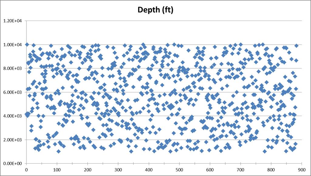
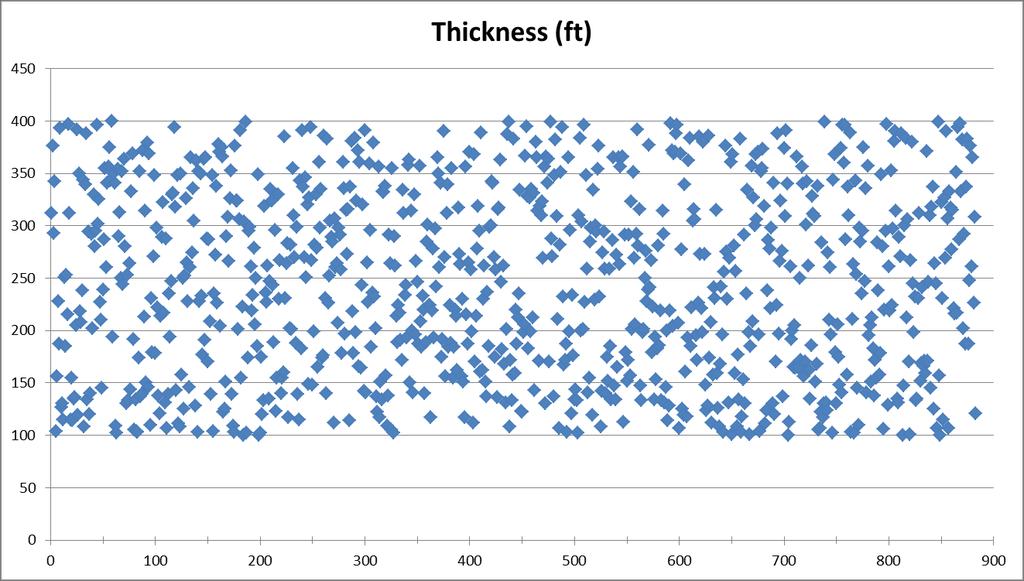
99 90

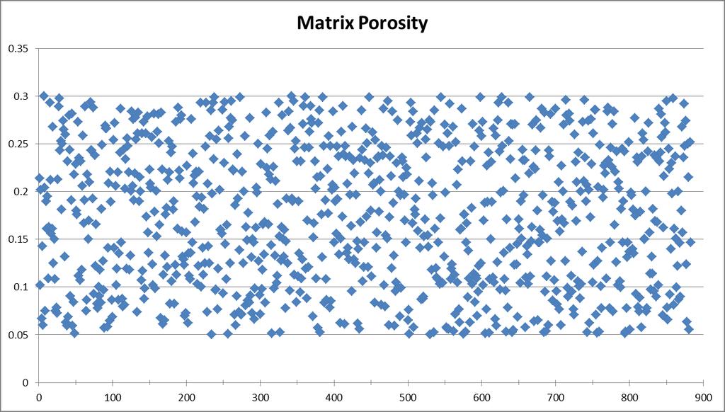
100 91

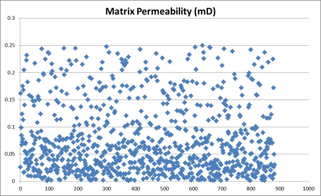
101 92

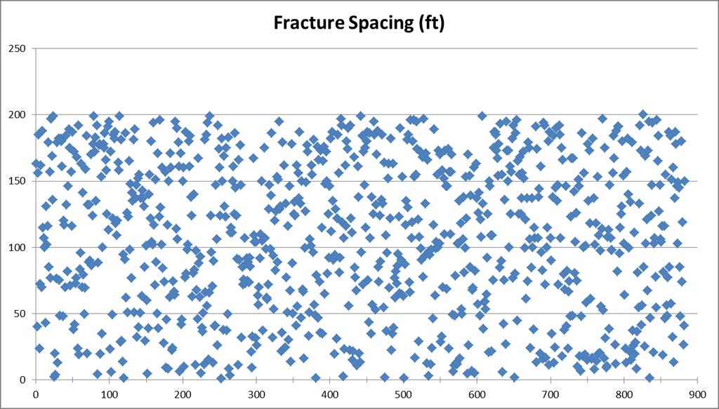
102 93

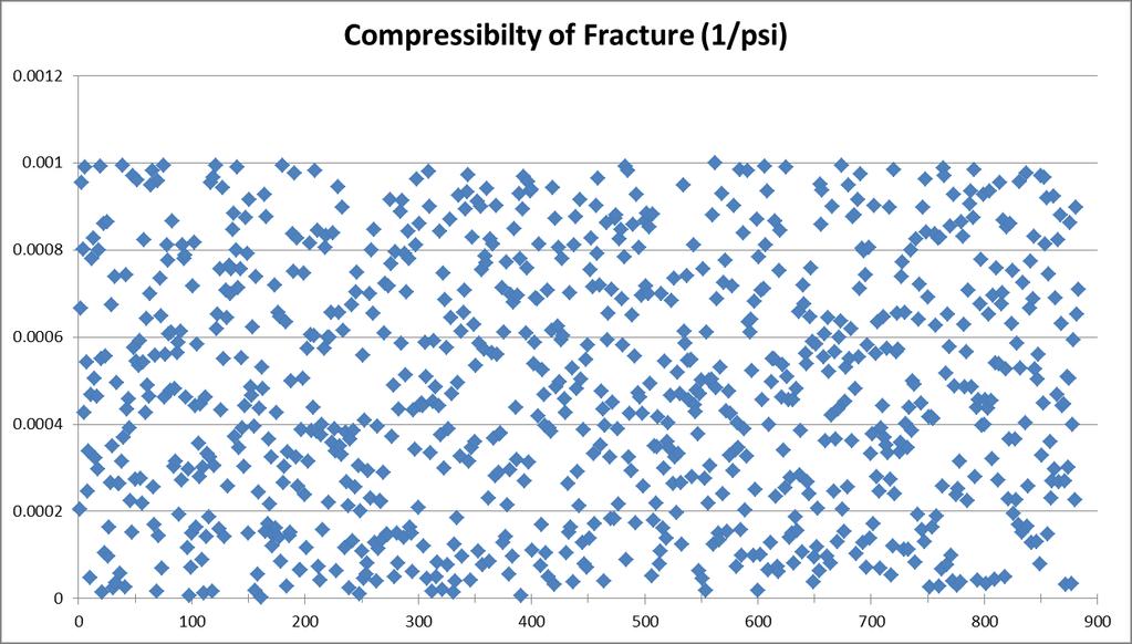
103 94

104 95 Appix C Curve Fitting Appix C-1 Exponential Curve Fitting clear clc t='times.xlsx'; gr='gasrate.xlsx'; time=xlsread(t); gasrate=xlsread(gr); %function [fitresult, gof] = createfitgasrateexp(timem, gasratemonthly) %CREATEFIT(TIMEM,GASRATEMONTHLY) % Create a fit. % % Data for 'createfitgasrate' fit: % X Input : time % Y Output: gasrate % Output: % fitresult : a fit object representing the fit. % gof : structure with goodness-of fit info. %