Text Compression. General remarks and Huffman coding Adobe pages Arithmetic coding Adobe pages 15 25
|
|
|
- Stella Penelope Poole
- 5 years ago
- Views:
Transcription
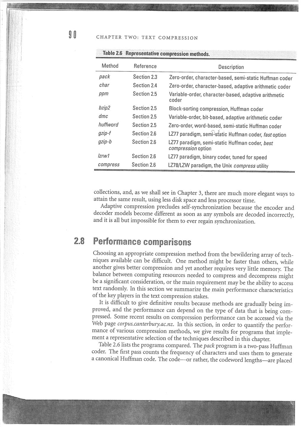
1 Text Compression General remarks and Huffman coding Adobe pages 2 14 Arithmetic coding Adobe pages Dictionary coding and the LZW family Adobe pages Performance considerations Adobe pages 47 57
2
3
4
5
6
7
8
9
10
11
12
13
14
15 Text Compression Arithmetic coding

16 Untitled 1 di 11 01/12/ Arithmetic Coding + Statistical Modeling = Data Compression Part 1 - Arithmetic Coding by Mark Nelson Dr. Dobb's Journal February, 1991 This page contains my original text and figures for the article that appeared in the February, 1991 DDJ. The article was originally written to be a 2 part feature, but was cut down to 1 part. Links to Part 2 are here and at the end of the article. Arithmetic Coding + Statistical Modeling = Data Compression Part 1 - Arithmetic Coding by Mark Nelson Most of the data compression methods in common use today fall into one of two camps: dictionary based schemes and statistical methods. In the world of small systems, dictionary based data compression techniques seem to be more popular at this time. However, by combining arithmetic coding with powerful modeling techniques, statistical methods for data compression can actually achieve better performance. This two-part article discusses how to combine arithmetic coding with several different modeling methods to achieve some impressive compression ratios. The first part of the article details how arithmetic coding works. The second shows how to develop some effective models that can use an arithmetic coder to generate high performance compression programs. Terms of Endearment Data compression operates in general by taking "symbols" from an input "text", processing them, and writing "codes" to a compressed file. For the purposes of this article, symbols are usually bytes, but they could just as easily be pixels, 80 bit floating point numbers, or EBCDIC characters. To be effective, a data compression scheme needs to be able to transform the compressed file back into an identical copy of the input text. Needless to say, it also helps if the compressed file is smaller than the input text! Dictionary based compression systems operate by replacing groups of symbols in the input text with fixed length codes. A well-known example of a dictionary technique is LZW data compression. (See "LZW Data Compression" in the 10/89 issue of DDJ). LZW operates by replacing strings of essentially unlimited length with codes that usually range in size from 9 to 16 bits. Statistical methods of data compression take a completely different approach. They operate by encoding symbols one at a time. The symbols are encoded into variable length output codes. The length of the output code varies based on the probability or frequency of the symbol. Low probability symbols are encoded using many bits, and high probability symbols are encoded using fewer bits. In practice, the dividing line between statistical and dictionary methods is not always so distinct. Some schemes can't be clearly put in one camp or the other, and there are always hybrids which use features from both techniques. However, the methods discussed in this article use arithmetic coding to implement purely statistical compression schemes.
17 Untitled 2 di 11 01/12/ Huffman Coding: The Retired Champion It isn't enough to just be able to accurately calculate the probability of characters in a datastream, we also need a coding method that effectively takes advantage of that knowledge. Probably the best known coding method based on probability statistics is Huffman coding. D. A. Huffman published a paper in 1952 describing a method of creating a code table for a set of symbols given their probabilities. The Huffman code table was guaranteed to produce the lowest possible output bit count possible for the input stream of symbols, when using fixed length codes. Huffman called these "minimum redundancy codes", but the scheme is now universally called Huffman coding. Other fixed length coding systems, such as Shannon-Fano codes, were shown by Huffman to be non-optimal. Huffman coding assigns an output code to each symbol, with the output codes being as short as 1 bit, or considerably longer than the input symbols, strictly depending on their probabilities. The optimal number of bits to be used for each symbol is the log base 2 of (1/p), where p is the probability of a given character. Thus, if the probability of a character is 1/256, such as would be found in a random byte stream, the optimal number of bits per character is log base 2 of 256, or 8. If the probability goes up to 1/2, the optimum number of bits needed to code the character would go down to 1. The problem with this scheme lies in the fact that Huffman codes have to be an integral number of bits long. For example, if the probability of a character is 1/3, the optimum number of bits to code that character is around 1.6. The Huffman coding scheme has to assign either 1 or 2 bits to the code, and either choice leads to a longer compressed message than is theoretically possible. This non-optimal coding becomes a noticeable problem when the probability of a character becomes very high. If a statistical method can be developed that can assign a 90% probability to a given character, the optimal code size would be 0.15 bits. The Huffman coding system would probably assign a 1 bit code to the symbol, which is 6 times longer than is necessary. Adaptive Schemes A second problem with Huffman coding comes about when trying to do adaptive data compression. When doing non-adaptive data compression, the compression program makes a single pass over the data to collect statistics. The data is then encoded using the statistics, which are unchanging throughout the encoding process. In order for the decoder to decode the compressed data stream, it first needs a copy of the statistics. The encoder will typically prepend a statistics table to the compressed message, so the decoder can read it in before starting. This obviously adds a certain amount of excess baggage to the message. When using very simple statistical models to compress the data, the encoding table tends to be rather small. For example, a simple frequency count of each character could be stored in as little as 256 bytes with fairly high accuracy. This wouldn't add significant length to any except the very smallest messages. However, in order to get better compression ratios, the statistical models by necessity have to grow in size. If the statistics for the message become too large, any improvement in compression ratios will be wiped out by added length needed to prepend them to the encoded message. In order to bypass this problem, adaptive data compression is called for. In adaptive data compression, both the encoder and decoder start with their statistical model in the same state. Each of them process a single character at a time, and update their models after the character is read in. This is very similar to the way most dictionary based schemes such as LZW coding work. A slight amount of efficiency is lost by beginning the message with a non-optimal model, but it is usually more than made up for by not having to pass any statistics with the message. The problem with combining adaptive modeling with Huffman coding is that rebuilding the Huffman tree is a very expensive process. For an adaptive scheme to be efficient, it is necessary to adjust the Huffman tree
18 Untitled 3 di 11 01/12/ after every character. Algorithms to perform adaptive Huffman coding were not published until over 20 years after Huffman coding was first developed. Even now, the best adaptive Huffman coding algorithms are still relatively time and memory consuming. Arithmetic Coding: how it works It has only been in the last ten years that a respectable candidate to replace Huffman coding has been successfully demonstrated: Arithmetic coding. Arithmetic coding completely bypasses the idea of replacing an input symbol with a specific code. Instead, it takes a stream of input symbols and replaces it with a single floating point output number. The longer (and more complex) the message, the more bits are needed in the output number. It was not until recently that practical methods were found to implement this on computers with fixed sized registers. The output from an arithmetic coding process is a single number less than 1 and greater than or equal to 0. This single number can be uniquely decoded to create the exact stream of symbols that went into its construction. In order to construct the output number, the symbols being encoded have to have a set probabilities assigned to them. For example, if I was going to encode the random message "BILL GATES", I would have a probability distribution that looks like this: Character Probability SPACE 1/10 A 1/10 B 1/10 E 1/10 G 1/10 I 1/10 L 2/10 S 1/10 T 1/10 Once the character probabilities are known, the individual symbols need to be assigned a range along a "probability line", which is nominally 0 to 1. It doesn't matter which characters are assigned which segment of the range, as long as it is done in the same manner by both the encoder and the decoder. The nine character symbol set use here would look like this: Character Probability Range SPACE 1/ A 1/ B 1/ E 1/ G 1/ I 1/ L 2/ S 1/ T 1/ Each character is assigned the portion of the 0-1 range that corresponds to its probability of appearance. Note also that the character "owns" everything up to, but not including the higher number. So the letter 'T' in fact has the range The most significant portion of an arithmetic coded message belongs to the first symbol to be encoded. When encoding the message "BILL GATES", the first symbol is "B". In order for the first character to be decoded properly, the final coded message has to be a number greater than or equal to 0.20 and less than What we do to encode this number is keep track of the range that this number could fall in. So after the first character is encoded, the low end for this range is 0.20 and the high end of the range is 0.30.
19 Untitled 4 di 11 01/12/ After the first character is encoded, we know that our range for our output number is now bounded by the low number and the high number. What happens during the rest of the encoding process is that each new symbol to be encoded will further restrict the possible range of the output number. The next character to be encoded, 'I', owns the range 0.50 through If it was the first number in our message, we would set our low and high range values directly to those values. But 'I' is the second character. So what we do instead is say that 'I' owns the range that corresponds to in the new subrange of This means that the new encoded number will have to fall somewhere in the 50th to 60th percentile of the currently established range. Applying this logic will further restrict our number to the range 0.25 to The algorithm to accomplish this for a message of any length is is shown below: Set low to 0.0 Set high to 1.0 While there are still input symbols do get an input symbol code_range = high - low. high = low + range*high_range(symbol) low = low + range*low_range(symbol) End of While output low Following this process through to its natural conclusion with our chosen message looks like this: New Character Low value High Value B I L L SPACE G A T E S So the final low value, will uniquely encode the message "BILL GATES" using our present encoding scheme. Given this encoding scheme, it is relatively easy to see how the decoding process will operate. We find the first symbol in the message by seeing which symbol owns the code space that our encoded message falls in. Since the number falls between 0.2 and 0.3, we know that the first character must be "B". We then need to remove the "B" from the encoded number. Since we know the low and high ranges of B, we can remove their effects by reversing the process that put them in. First, we subtract the low value of B from the number, giving Then we divide by the range of B, which is 0.1. This gives a value of We can then calculate where that lands, which is in the range of the next letter, "I". The algorithm for decoding the incoming number looks like this: get encoded number Do find symbol whose range straddles the encoded number output the symbol range = symbol low value - symbol high value subtract symbol low value from encoded number divide encoded number by range until no more symbols
20 Untitled 5 di 11 01/12/ Note that I have conveniently ignored the problem of how to decide when there are no more symbols left to decode. This can be handled by either encoding a special EOF symbol, or carrying the stream length along with the encoded message. The decoding algorithm for the "BILL GATES" message will proceed something like this: Encoded Number Output Symbol Low High Range B I L L SPACE G A T E S In summary, the encoding process is simply one of narrowing the range of possible numbers with every new symbol. The new range is proportional to the predefined probability attached to that symbol. Decoding is the inverse procedure, where the range is expanded in proportion to the probability of each symbol as it is extracted. Practical Matters The process of encoding and decoding a stream of symbols using arithmetic coding is not too complicated. But at first glance, it seems completely impractical. Most computers support floating point numbers of up to 80 bits or so. Does this mean you have to start over every time you finish encoding 10 or 15 symbols? Do you need a floating point processor? Can machines with different floating point formats communicate using arithmetic coding? As it turns out, arithmetic coding is best accomplished using standard 16 bit and 32 bit integer math. No floating point math is required, nor would it help to use it. What is used instead is a an incremental transmission scheme, where fixed size integer state variables receive new bits in at the low end and shift them out the high end, forming a single number that can be as many bits long as are available on the computer's storage medium. In the previous section, I showed how the algorithm works by keeping track of a high and low number that bracket the range of the possible output number. When the algorithm first starts up, the low number is set to 0.0, and the high number is set to 1.0. The first simplification made to work with integer math is to change the 1.0 to , or in binary. In order to store these numbers in integer registers, we first justify them so the implied decimal point is on the left hand side of the word. Then we load as much of the initial high and low values as will fit into the word size we are working with. My implementation uses 16 bit unsigned math, so the initial value of high is 0xFFFF, and low is 0. We know that the high value continues with FFs forever, and low continues with 0s forever, so we can shift those extra bits in with impunity when they are needed. If you imagine our "BILL GATES" example in a 5 digit register, the decimal equivalent of our setup would look like this: HIGH: LOW: 00000
21 Untitled 6 di 11 01/12/ In order to find our new range numbers, we need to apply the encoding algorithm from the previous section. We first had to calculate the range between the low value and the high value. The difference between the two registers will be , not This is because we assume the high register has an infinite number of 9's added on to it, so we need to increment the calculated difference. We then compute the new high value using the formula from the previous section: high = low + high_range(symbol) In this case the high range was.30, which gives a new value for high of Before storing the new value of high, we need to decrement it, once again because of the implied digits appended to the integer value. So the new value of high is The calculation of low follows the same path, with a resulting new value of So now high and low look like this: HIGH: (999...) LOW: (000...) At this point, the most significant digits of high and low match. Due to the nature of our algorithm, high and low can continue to grow closer to one another without quite ever matching. This means that once they match in the most significant digit, that digit will never change. So we can now output that digit as the first digit of our encoded number. This is done by shifting both high and low left by one digit, and shifting in a 9 in the least significant digit of high. The equivalent operations are performed in binary in the C implementation of this algorithm. As this process continues, high and low are continually growing closer together, then shifting digits out into the coded word. The process for our "BILL GATES" message looks like this: HIGH LOW RANGE CUMULATIVE OUTPUT Initial state Encode B ( ) Shift out Encode I ( ) Shift out Encode L ( ) Encode L ( ) Shift out Encode SPACE ( ) Shift out Encode G ( ) Shift out Encode A ( ) Shift out Encode T ( ) Shift out Encode E ( ) Shift out Encode S ( ) Shift out Shift out Shift out Note that after all the letters have been accounted for, two extra digits need to be shifted out of either the high or low value to finish up the output word.
22 Untitled 7 di 11 01/12/ A Complication This scheme works well for incrementally encoding a message. There is enough accuracy retained during the double precision integer calculations to ensure that the message is accurately encoded. However, there is potential for a loss of precision under certain circumstances. In the event that the encoded word has a string of 0s or 9s in it, the high and low values will slowly converge on a value, but may not see their most significant digits match immediately. For example, high and low may look like this: High: Low: At this point, the calculated range is going to be only a single digit long, which means the output word will not have enough precision to be accurately encoded. Even worse, after a few more iterations, high and low could look like this: High: Low: At this point, the values are permanently stuck. The range between high and low has become so small that any calculation will always return the same values. But, since the most significant digits of both words are not equal, the algorithm can't output the digit and shift. It seems like an impasse. The way to defeat this underflow problem is to prevent things from ever getting this bad. The original algorithm said something like "If the most significant digit of high and low match, shift it out". If the two digits don't match, but are now on adjacent numbers, a second test needs to be applied. If High and low are one apart, we then test to see if the 2nd most significant digit in high is a 0, and the 2nd digit in low is a 9. If so, it means we are on the road to underflow, and need to take action. When underflow rears its ugly head, we head it off with a slightly different shift operation. Instead of shifting the most significant digit out of the word, we just delete the 2nd digits from high and low, and shift the rest of the digits left to fill up the space. The most significant digit stays in place. We then have to set an underflow counter to remember that we threw away a digit, and we aren't quite sure whether it was going to end up as a 0 or a 9. The operation looks like this: Before After High: Low: Underflow: 0 1 After every recalculation operation, if the most significant digits don't match up, we can check for underflow digits again. If they are present, we shift them out and increment the counter. When the most significant digits do finally converge to a single value, we first output that value. Then, we output all of the "underflow" digits that were previously discarded. The underflow digits will be all 9s or 0s, depending on whether High and Low converged to the higher or lower value. In the C implementation of this algorithm, the underflow counter keeps track of how many ones or zeros to put out. Decoding In the "ideal" decoding process, we had the entire input number to work with. So the algorithm has us do
23 Untitled 8 di 11 01/12/ things like "divide the encoded number by the symbol probability." In practice, we can't perform an operation like that on a number that could be billions of bytes long. Just like the encoding process, the decoder can operate using 16 and 32 bit integers for calculations. Instead of maintaining two numbers, high and low, the decoder has to maintain three integers. The first two, high and low, correspond exactly to the high and low values maintained by the encoder. The third number, code, contains the current bits being read in from the input bits stream. The code value will always lie in between the high and low values. As they come closer and closer to it, new shift operations will take place, and high and low will move back away from code. The high and low values in the decoder correspond exactly to the high and low that the encoder was using. They will be updated after every symbol just as they were in the encoder, and should have exactly the same values. By performing the same comparison test on the upper digit of high and low, the decoder knows when it is time to shift a new digit into the incoming code. The same underflow tests are performed as well, in lockstep with the encoder. In the ideal algorithm, it was possible to determine what the current encoded symbols was just by finding the symbol whose probabilities enclosed the present value of the code. In the integer math algorithm, things are somewhat more complicated. In this case, the probability scale is determined by the difference between high and low. So instead of the range being between 0.0 and 1.0, the range will be between two positive 16 bit integer counts. The current probability is determined by where the present code value falls along that range. If you were to divide (value-low) by (high-low+1), you would get the actual probability for the present symbol. Where's the Beef? So far, this encoding process may look interesting, but it is not immediately obvious why it is an improvement over Huffman coding. The answer becomes clear when we examine a case where the probabilities are a little different. Lets examine the case where we have to encode the stream "AAAAAAA", and the probability of "A" is known to be This means there is a 90% chance that any incoming character will be the letter "A". We set up our probability table so that the letter "A" occupies the range 0.0 to 0.9, and the End of message symbol occupies the 0.9 to 1.0 range. The encoding process then looks like this: New Character Low value High Value A A A A A A A END Now that we know what the range of low and high values are, all that remains is to pick a number to encode this message. The number "0.45" will make this message uniquely decode to "AAAAAAA". Those two decimal digits take slightly less than 7 bits to specify, which means that we have encoded eight symbols in less than 8 bits! An optimal Huffman coded message would have taken a minimum of 9 bits using this scheme. To take this point even further, I set up a test that had only two symbols defined. The byte value '0' had a 16382/16383 probability, and an EOF symbol had a 1/16383 probability of occurring. I then created a test file which was filled with 100,000 '0's. After compression using this model, the output file was only 3 bytes long! The minimum size using Huffman coding would have been 12,501 bytes. This is obviously a
24 Untitled 9 di 11 01/12/ contrived example, but it does illustrate the point that arithmetic coding is able to compress data at rates much better than 1 bit per byte when the symbol probabilities are right. The Code An encoding procedure written in C is shown in listing 1 and 2. It contains two parts, an initialization procedure, and the encoder routine itself. The code for the encoder as well as the decoder were first published in an article entitled "Arithmetic Coding for Data Compression" in the February 1987 issue of "Communications of the ACM", by Ian H. Witten, Radford Neal, and John Cleary, and is being published here with the author's permission. I have modified the code slightly so as to further isolate the modeling and coding portions of the program. There are two major differences between the algorithms shown earlier and the code in listing 1-2. The first difference is in the way probabilities are transmitted. In the algorithms shown above, the probabilities were kept as a pair of floating point numbers on the 0.0 to 1.0 range. Each symbol had its own section of that range. In the programs that are shown here, a symbol has a slightly different definition. Instead of two floating point numbers, the symbol's range is defined as two integers, which are counts along a scale. The scale is also included as part of the symbol definition. So, for the "BILL GATES" example, the letter L was defined previously as the high/low pair of 0.60 and In the code being used here, "B" would be defined as the low and high counts of 6 and 8, with the symbol scale being 10. The reason it is done this way is because it fits in well with the way we keep statistics when modeling this type of data. The two methods are equivalent, it is just that keeping integer counts cuts down on the amount of work needing to be done. Note that the character actually owns the range up to but not including the high value. The second difference in this algorithm is that all of the comparison and shifting operations are being done in base 2, rather than base 10. The illustrations given previously were done on base 10 numbers to make the algortihms a little more comprehensible. The algorithms work properly in base 10, but masking off digits and shifting in base 10 on most computers is difficult. So instead of comparing the top two digits, we now compare the top two bits. There are two things missing that are needed in order to use the encoding and decoding algorithms. The first is a set of bit oriented input and output routines. These are shown in listing 3 and 4, and are presented here without comment. The modeling code is responsible for keeping track of the probabilities of each character, and performing two different transformations. During the encoding process, the modeling code has to take a character to be encoded and convert it to a probability range. The probability range is defined as a low count, a high count, and a total range. During the decoding process, the modeling code has to take a count derived from the input bit stream and convert it into a character for output. Test Code A short test program is shown Listing 3. It implements a compression/expansion program that uses the "BILL GATES" model discussed previously. Adding a few judiciously placed print statements will let you track exactly what is happening in this program. BILL.C has its own very simple modeling unit, which has a set of fixed probabilities for each of the possible letters in the message. I added a new character, the null string terminator, so as to know when to stop decoding the message. BILL.C encodes an arbitrarily defined input string, and writes it out to a file called TEST.CMP. It then decodes the message and prints it to the screen for verification. There are a few functions in BILL.C that are modeling functions, which haven't been discussed yet. During the encoding process, a routine called convert_int_to_symbol is called. This routine gets a given input character, and converts it to a low count, high count, and scale using the current model. Since our model for BILL.C is a set of fixed probabilities, this just means looking up the probabilities in the table. Once those are defined, the encoder can be called.
25 Untitled 10 di 11 01/12/ During the decoding process, there are two functions associated with modeling. In order to determine what character is waiting to be decoded on the input stream, the model needs to be interrogated to determine what the present scale is. In our example, the scale (or range of counts) is fixed at 11, since there are always 11 counts in our model. This number is passed to the decoding routine, and it returns a count for the given symbol using that scale. Then, a modeling function called convert_symbol_to_int is called. It takes the given count, and determines what character matches the count. Finally, the decoder is called again to process that character out of the input stream. Next Time Once you successfully understand how to encode/decode symbols using arithmetic coding, you can then begin trying to create models that will give superior compression performance. Next month's concluding article discusses some of the methods you can try for adaptive compression. A fairly simple statistical modeling program is able to provide compression superior to respected programs such as PKZIP or COMPRESS. References As I mentioned previously, the article in the June 1987 "Communications of the ACM" provides the definitive overview of arithmetic coding. Most of the article is reprinted in the book "Text Compression", by Timothy C. Bell, John G. Cleary, and Ian H. Witten. This book provides an excellent overview of both statistical and dictionary based compression techniques. Another good book is "Data Compression" by James Storer. Bell, Timothy C., Cleary, John G., Witten, Ian H, (1990) "Text Compression", Prentice Hall, Englewood NJ Nelson, Mark (1989) "LZW Data Compression", Doctor Dobb's Journal, October, pp Storer, J.A., (1988) "Data Compression", Computer Science Press, Rockville, MD Witten, Ian H., Neal, Radford M., and Cleary, John G. (1987) "Arithmetic Coding for Data Compression", Communications of the ACM, June, pp Listing 1 coder.h Constants, declarations, and prototypes needed to use the arithmetic coding routines. These declarations are for routines that need to interface with the arithmetic coding stuff in coder.c Listing 2 coder.c This file contains the code needed to accomplish arithmetic coding of a symbol. All the routines in this module need to know in order to accomplish coding is what the probabilities and scales of the symbol counts are. This information is generally passed in a SYMBOL structure. Listing 3 bitio.h This header file contains the function prototypes needed to use the bitstream i/o routines. Listing 4 bitio.c This routine contains a set of bit oriented i/o routines used for arithmetic data compression. Listing 5 bill.c This short demonstration program will use arithmetic data compression to encode and then decode a string that only uses the letters out of the phrase "BILL GATES". It uses a fixed, hardcoded table of probabilities. Continue with Part 2: Statistical Modeling
26 Text Compression Dictionary models
27
28
29
30
31
32
33
34
35
36
37
38 Text Compression Another view of the LZW family

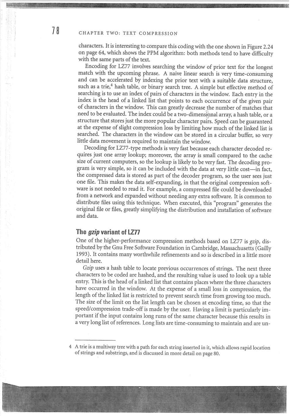
 and raster images (code words represent pixels). All the dictionary methods can be subdivided into two main groups.")
39 Data Compression Reference Center Pagina 1 di 8 01/12/2008 Project Algorithms Research Resources Forum prevlnext \home\algorithms\ Dictionary methods LZ77 LZSS LZ78 LZW Dictionary methods Books References Related links These compression methods use the property of many data types to contain repeating code sequences. Good examples of such data are text files (code words represent characters) and raster images (code words represent pixels). All the dictionary methods can be subdivided into two main groups. The methods of the first group try to find if the character sequence currently being compressed has already occurred earlier in the input data and then, instead of repeating it, output only a po inter to the earlier occurrence. This is illustrated in the following diagram: The dictionary here is implicit -- it is represented by the previously processed data. All the methods of this group are based on the algorithm developed and published in 1977 by Abraham Lempel and Jakob Ziv -- LZ77. A refineme nt of this algorithm which is the basis for practically all the later methods in this group is the LZSS algorithm developed in 1982 by Storer and Szymanski. The algorithms of the second group create a dictionary of the phrases that occurr in the input data. When they encounter a phrase already present in the dictionary, they just output the index number of the phrase in t he dictionary. This is explained in the diagram below:

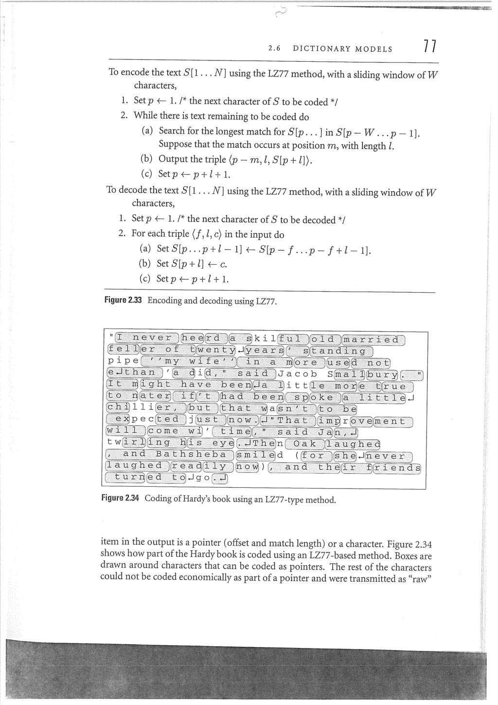
40 Data Compression Reference Center Pagina 2 di 8 These methods are based on the algorithm developed and published by Lempel and Ziv in LZ78. The refinement which is the basis for the later methods is called LZW. It was developed by Terry Welch i n 1984 for hardware implementation in high-performance disk controllers. back to top The LZ77 algorithm Terms used in the algorithm: Input stream: the sequence of characters to be compressed; Character: the basic data element in the input stream; Coding position: the position of the character in the input stream that is currently being coded (the beginning of the lookahead buffer); Lookahead buffer: the character sequence from the coding position to the end of the input stream; The Window of size W contains W characters from the coding position backwards, i.e. the last W processed characters; A Pointer points to the match in the window and also specifies its length. The principle of encoding The algorithm searches the window for the longest match with the beginning of the lookahead buffer and outputs a pointer to that match. Since it is possible that not even a one-character match can be found, the output cannot contain just pointers. LZ77 solves this problem this way: after each pointer it outputs the first character in the lookahead buffer after the match. If there is no match, it outputs a null-pointer and the character at the coding position. The encoding algorithm Set the coding position to the beginning of the input stream; 1. find the longest match in the window for the lookahead buffer; 2. output the pair (P,C) with the following meaning: P is the pointer to the match in the window; C is the first character in the lookahead buffer that didn't match; 3. if the lookahead buffer is not empty, move the coding position (and the window) L+1 characters forward and return to step 2. An example The encoding process is presented in Table 1. The column Step indicates the number of the encoding step. It completes each time the encoding algorithm makes an output. With LZ77 this happens in each pass through the step 3. The column Pos indicates the coding position. The first character in the input stream has the coding position /12/2008
41 Data Compression Reference Center Pagina 3 di 8 The column Match shows the longest match found in the window. The column Char shows the first character in the lookahead buffer after the match. The column Output presents the output in the format (B,L) C: (B,L) is the pointer (P) to the Match. This gives the following instruction to the decoder: "Go back B characters in the window and copy L characters to the output"; C is the explicit Character. Input stream for encoding: Pos Char A A B C B B A B C Table 1: The encoding process Step Pos Match Char Output A (0,0) A 2. 2 A B (1,1) B C (0,0) C 4. 5 B B (2,1) B 5. 7 A B C (5,2) C Decoding The window is maintained the same way as while encoding. In each step the algorithm reads a pair (P,C) from the input. It outputs the sequence from the window specified by P and the character C. Practical characteristics The compression ratio this method achieves is very good for many types of data, but the encoding can be quite time-consuming, since there is a lot of comparisons to perform between the lookahead buffer and the window. On the other hand, the decoding is very simple and fast. Memory requirements are low both for the encoding and the decoding. The only structure held in memory is the window, which is usually sized between 4 and 64 kilobytes. back to top The LZSS Algorithm Difference to the LZ77 The algorihtm LZ77 solves the case of no match in the window by outputting an explicit character after each pointer. This solution contains redundancy: either is the null-pointer redundant, or the extra character that could be included in the next match. The LZSS algorithm solves this problem in a more efficient manner: the pointer is output only if it points to a match longer than the pointer itself; otherwise, explicit characters are sent. Since the output stream now contains assorted pointers and characters, each of them has to have an extra ID-bit which discriminates between them. The encoding algorithm 1. Place the coding position to the beginning of the input stream; 2. find the longest match in the window for the lookahead buffer: P := pointer to this match; L := length of the match; 3. is L >= MIN_LENGTH? YES: output P and move the coding position L characters forward; NO: output the first character of the lookahead buffer and move the coding positon one character forward; 4. if there are more characters in the input stream, go back to step 2. An example The encoding process is presented in Table 1. The column Step indicates the number of the encoding step. It completes each time the encoding algorithm makes an output. With LZSS this happens in each pass through the step 3. The column Pos indicates the coding position. The first character in the input stream has the coding position 1. The column Match shows the longest match found in the window. The column Output presents the output, which can be one of the following: A pointer to the Match, in the format (B,L). This gives the following instruction to the decoder: "Go back B characters in the window and copy L characters to the output"; The Match itself in explicit form (if it is only one character long, since MIN_LENGTH is set to 2) Input stream for encoding: Pos Char A A B B C B B A A B C 01/12/2008
42 Data Compression Reference Center Pagina 4 di 8 Table 1: The encoding process (MIN_LENGTH = 2) Step Pos Match Output A 2 2 A A B 4 4 B B C 6 6 B B (3,2) 7 8 A A B (7,3) 8 11 C C Decoding The window is slid over the output stream in the same manner the encoding algorithm slides it over the input stream. Explicit characters are output directly, and when a pointer is encountered, the string in the window it points to is output. Performance comparison to LZ77 This algorithm generally yields a better compression ratio than LZ77 with practically the same processor and memory requirements. The decoding is still extremely simple and quick. That's why it has become the basis for practically all the later algorithms of this type. Implementations It is implemented in almost all of the popular archivers: PKZip, ARJ, LHArc, ZOO etc. Of course, every archiver implements it a bit differently, depending on the pointer length (it can also be variable), the window size, the way it is moved (some implementations move the window in N-character steps) and so on. LZSS can also be combined with the entropy coding methods: for example, ARJ applies Huffman encoding, and PKZip 1.x applies Shannon-Fano encoding (later versions of PKZip also apply Huffman encoding). back to top The LZ78 algorithm Terms used in the algorithm Charstream: a sequence of data to be encoded; Character: the basic data element in the charstream; Prefix: a sequence of characters that precede one character; String: the prefix together with the character it precedes; Code word: a basic data element in the codestream. It represents a string from the dictionary; Codestream: the sequence of code words and characters (the output of the encoding algorithm); Dictionary: a table of strings. Every string is assigned a code word according to its index number in the dictionary; Current prefix: the prefix currently being processed in the encoding algorithm. Symbol: P; Current character: a character determined in the endocing algorithm. Generally this is the character preceded by the current prefix. Symbol: C. Current code word: the code word currently processed in the decoding algorithm. It is signified by W, and the string which it denotes by string.w. Encoding At the beginning of encoding the dictionary is empty. In order to explain the principle of encoding, let's consider a point within the encoding process, when the dictionary already contains some strings. We start analyzing a new prefix in the charstream, beginning with an empty prefix. If its corresponding string (prefix + the character after it -- P+C) is present in the dictionary, the prefix is extended with the character C. This extending is repeated until we get a string which is not present in the dictionary. At that point we output two things to the codestream: the code word that represents the prefix P, and then the character C. Then we add the whole string (P+C) to the dictionary and start processing the next prefix in the charstream. A special case occurs if the dictionary doesn't contain even the starting one-character string (for example, this always happens in the first encoding step). In that case we output a special code word that represents an empty string, followed by this character and add this character to the dictionary. The output from this algorithm is a sequence of code word-character pairs (W,C). Each time a pair is output to the codestream, the string from the dictionary corresponding to W is extended with the character C and the resulting string is added to the dictionary. This means that when a new string is being added, the dictionary already contains all the substrings formed by removing characters from the end of the new string. The encoding algorithm 01/12/2008
43 Data Compression Reference Center Pagina 5 di 8 1. At the start, the dictionary and P are empty; 2. C := next character in the charstream; 3. Is the string P+C present in the dictionary? a. if it is, P := P+C (extend P with C); b. if not, i. output these two objects to the codestream: the code word corresponding to P (if P is empty, output a zero); C, in the same form as input from the charstream; ii. add the string P+C to the dictionary; iii. P := empty; c. are there more characters in the charstream? if yes, return to step 2; if not: i. if P is not empty, output the code word corresponding to P; ii. END. Decoding At the start of decoding the dictionary is empty. It gets reconstructed in the process of decoding. In each step a pair code wordcharacter -- (W,C) is read from the codestream. The code word always refers to a string already present in the dictionary. The string.w and C are output to the charstream and the string (string.w+c) is added to the dictionary. After the decoding, the dictionary will look exactly the same as after the encoding. The decoding algorithm 1. At the start the dictionary is empty; 2. W := next code word in the codestream; 3. C := the character following it; 4. output the string.w to the codestream (this can be an empty string), and then output C; 5. add the string.w+c to the dictionary; 6. are there more code words in the codestream? if yes, go back to step 2; if not, END. An example The encoding process is presented in Table 1. The column Step indicates the number of the encoding step. Each encoding step is completed when the step 3.b. in the encoding algorithm is executed. The column Pos indicates the current position in the input data. The column Dictionary shows what string has been added to the dictionary. The index of the string is equal to the step number. The column Output presents the output in the form (W,C). The output of each step decodes to the string that has been added to the dictionary. Charstream to be encoded: Pos Char A B B C B C A B A Table 1: The encoding process Step Pos Dictionary Output 1. 1 A (0,A) 2. 2 B (0,B) 3. 3 B C (2,C) 4. 5 B C A (3,A) 5. 8 B A (2,A) Practical characteristics The biggest advantage over the LZ77 algorithm is the reduced number of string comparisons in each encoding step. The compression ratio is similar to the LZ77. Since the derived method, LZW, is much more popular, you should see there for further info. back to top The LZW algorithm In this algorithm, the same terms are used as in LZ78, with the following addendum: A Root is a single-character string. 01/12/2008
44 Data Compression Reference Center Pagina 6 di 8 Differences to the LZ78 in the principle of encoding Only code words are output. This means that the dictionary cannot be empty at the start: it has to contain all the individual characters (roots) that can occurr in the charstream; Since all possible one-character strings are already in the dictionary, each encoding step begins with a one-character prefix, so the first string searched for in the dictionary has two characters; The character with which the new prefix starts is the last character of the previous string (C). This is necessary to enable the decoding algorihtm to reconstruct the dictionary without the help of explicit characters in the codestream. The encoding algorithm 1. At the start, the dictionary contains all possible roots, and P is empty; 2. C := next character in the charstream; 3. Is the string P+C present in the dictionary? a. if it is, P := P+C (extend P with C); b. if not, i. output the code word which denotes P to the codestream; ii. add the string P+C to the dictionary; iii. P := C (P now contains only the character C); c. are there more characters in the charstream? if yes, go back to step 2; if not: i. output the code word which denotes P to the codestream; ii. END. Decoding: additional terms Current code word: the code word currently being processed. It's signified with cw, and the string it denotes with string.cw; Previous code word: the code word that precedes the current code word in the codestream. It's signified with pw, and the string it denotes with string.pw. The principle of decoding At the start of decoding, the dictionary looks the same as at the start of encoding -- it contains all possible roots. Let's consider a point in the process of decoding, when the dictionary contains some longer strings. The algorithm remembers the previous code word (pw) and then reads the current code word (cw) from the codestream. It outputs the string.cw, and adds the string.pw extended with the first character of the string.cw to the dictionary. This is the character that would have been explicitly read from the codestream in LZ78. Because of this principle, the decoding algorithm "lags" one step behind the encoding algorithm with the adding of new strings to the dictionary. A special case occurrs if the cw denotes an empty entry in the dictionary. This can happen because of the explained "lagging" behind the encoding algorithm. It happens if the encoding algorithm reads the string that it has just added to the dictionary in the previous step. During the decoding this string is not yet present in the dictionary. A string can occurr twice in a row in the charstream only if its first and last character are equal, because the next string always starts with the last character of the previous one. This leads to the following decoding rule: the string.pw is extended with its own first character and the resulting string is added to the dictionary and output to the charstream. The decoding algorithm 1. At the start the dictionary contains all possible roots; 2. cw := the first code word in the codestream (it denotes a root); 3. output the string.cw to the charstream; 4. pw := cw; 5. cw := next code word in the codestream; 6. Is the string.cw present in the dictionary? if it is, 1. output the string.cw to the charstream; 2. P := string.pw; 3. C := the first character of the string.cw; 4. add the string P+C to the dictionary; if not, 1. P := string.pw; 2. C := the first character of the string.pw; 3. output the string P+C to the charstream and add it to the dictionary (now it corresponds to the cw); 7. Are there more code words in the codestream? if yes, go back to step 4; if not, END. An example The encoding process is presented in Table 1. The column Step indicates the number of the encoding step. Each encoding step is completed when the step 3.b. in the encoding algorithm is executed. 01/12/2008
45 Data Compression Reference Center Pagina 7 di 8 The column Pos indicates the current position in the input data. The column Dictionary shows the string that has been added to the dictionary and its index number in brackets. The column Output shows the code word output in the corresponding encoding step. Contents of the dictionary at the beginning of encoding: (1) A (2) B (3) C Charstream to be encoded: Pos Char A B B A B A B A C Table 1: The encoding process Step Pos Dictionary Output 1. 1 (4) A B (1) 2. 2 (5) B B (2) 3. 3 (6) B A (2) 4. 4 (7) A B A (4) 5. 6 (8) A B A C (7) (3) Table 2. explains the decoding process. In each decoding step the algorithm reads one code word (Code), outputs the corresponding string (Output) and adds a string to the dictionary (Dictionary). Table 2: The decoding process Step Code Output Dictionary 1. (1) A (2) B (4) A B 3. (2) B (5) B B 4. (4) A B (6) B A 5. (7) A B A (7) A B A 6. (3) C (8) A B A C Let's analyze the step 4. The previous code word (2) is stored in pw, and cw is (4). The string.cw is output ("A B"). The string.pw ("B") is extended with the first character of the string.cw ("A") and the result ("B A") is added to the dictionary with the index (6). We come to the step 5. The content of cw=(4) is copied to pw, and the new value for cw is read: (7). This entry in the dictionary is empty. Thus, the string.pw ("A B") is extended with its own first character ("A") and the result ("A B A") is stored in the dictionary with the index (7). Since cw is (7) as well, this string is also sent to the output. Practical characteristics This method is very popular in practice. Its advantage over the LZ77-based algorithms is in the speed because there are not that many string comparisons to perform. Further refinements add variable code word size (depending on the current dictionary size), deleting of the old strings in the dictionary etc. For example, these refinements are used in the GIF image format and in the UNIX compress utility for general compression. Another interesting variation is the LZMW algorithm. It forms a new entry in the dictionary by concatenating the two previous ones. This enables a faster buildup of longer strings. The LZW method is patented -- the owner of the patent is the Unisys company. It allows free use of the method, except for the producers of commercial software. back to top Books 1. Mark Nelson "The Data Compression Book" 2. Morgan Kaufmann "Introduction to Data Compression" 01/12/2008
46 Data Compression Reference Center Pagina 8 di 8 3. Khalid Sayood "Introduction to Data Compression" 4. David Solomon "Data Compression : The Complete Reference" 5. Peter Wayner "Compression alg. for real programers (for real programmers)" 6. Other books at Amazon.com back to top References J.Ziv and A.Lempel "A Universal Algorithm for sequential Data compression" "IEEE Transactions on Information theory" Vol IT-23, No.3, May 1977, PP Morgan Kaufmann "Introduction to Data Compression" Terry Welch "A Technique for High Performance Data Compression" "IEEE Computer" Vol 17, No. 6, 1984, PP Mark Nelson "The Data Compression Book" Timothy C. Bell, John G. Cleary, and Ian H. Witten "Text Compression" 1990 back to top Related Links 1. Lempel-Ziv compression algorithms 2. Lempel-Ziv-Welch Compression (LZW) 3. Lempel-Ziv compression of a file 4. Other links (Yahoo) back to top Copyright Data Compression Reference Center (compresswww@rasip.fer.hr) 01/12/2008
47 Text Compression Performance considerations
48
49
50
51
52
53
54
55
56
57
THE RELATIVE EFFICIENCY OF DATA COMPRESSION BY LZW AND LZSS
 THE RELATIVE EFFICIENCY OF DATA COMPRESSION BY LZW AND LZSS Yair Wiseman 1* * 1 Computer Science Department, Bar-Ilan University, Ramat-Gan 52900, Israel Email: wiseman@cs.huji.ac.il, http://www.cs.biu.ac.il/~wiseman
Dictionary techniques
 Dictionary techniques The final concept that we will mention in this chapter is about dictionary techniques. Many modern compression algorithms rely on the modified versions of various dictionary techniques.
EE-575 INFORMATION THEORY - SEM 092
 EE-575 INFORMATION THEORY - SEM 092 Project Report on Lempel Ziv compression technique. Department of Electrical Engineering Prepared By: Mohammed Akber Ali Student ID # g200806120. ------------------------------------------------------------------------------------------------------------------------------------------
Entropy Coding. - to shorten the average code length by assigning shorter codes to more probable symbols => Morse-, Huffman-, Arithmetic Code
 Entropy Coding } different probabilities for the appearing of single symbols are used - to shorten the average code length by assigning shorter codes to more probable symbols => Morse-, Huffman-, Arithmetic
Engineering Mathematics II Lecture 16 Compression
 010.141 Engineering Mathematics II Lecture 16 Compression Bob McKay School of Computer Science and Engineering College of Engineering Seoul National University 1 Lossless Compression Outline Huffman &
Comparative Study of Dictionary based Compression Algorithms on Text Data
 88 Comparative Study of Dictionary based Compression Algorithms on Text Data Amit Jain Kamaljit I. Lakhtaria Sir Padampat Singhania University, Udaipur (Raj.) 323601 India Abstract: With increasing amount
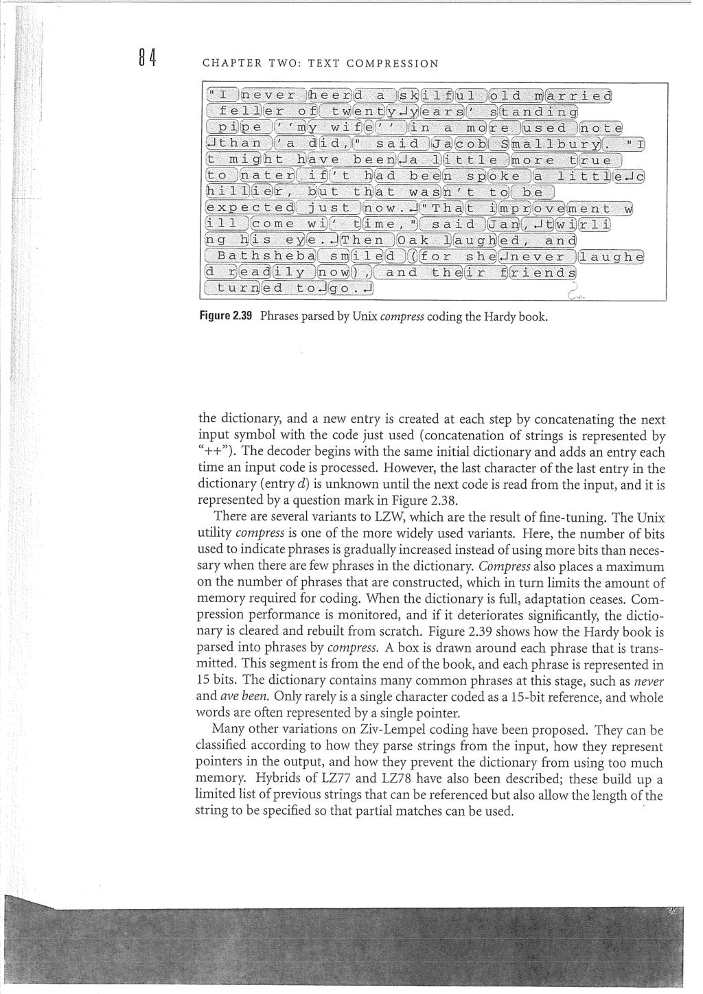
SIGNAL COMPRESSION Lecture Lempel-Ziv Coding
 SIGNAL COMPRESSION Lecture 5 11.9.2007 Lempel-Ziv Coding Dictionary methods Ziv-Lempel 77 The gzip variant of Ziv-Lempel 77 Ziv-Lempel 78 The LZW variant of Ziv-Lempel 78 Asymptotic optimality of Ziv-Lempel
CS 493: Algorithms for Massive Data Sets Dictionary-based compression February 14, 2002 Scribe: Tony Wirth LZ77
 CS 493: Algorithms for Massive Data Sets February 14, 2002 Dictionary-based compression Scribe: Tony Wirth This lecture will explore two adaptive dictionary compression schemes: LZ77 and LZ78. We use the
An Asymmetric, Semi-adaptive Text Compression Algorithm
 An Asymmetric, Semi-adaptive Text Compression Algorithm Harry Plantinga Department of Computer Science University of Pittsburgh Pittsburgh, PA 15260 planting@cs.pitt.edu Abstract A new heuristic for text
Analysis of Parallelization Effects on Textual Data Compression
 Analysis of Parallelization Effects on Textual Data GORAN MARTINOVIC, CASLAV LIVADA, DRAGO ZAGAR Faculty of Electrical Engineering Josip Juraj Strossmayer University of Osijek Kneza Trpimira 2b, 31000
FPGA based Data Compression using Dictionary based LZW Algorithm
 FPGA based Data Compression using Dictionary based LZW Algorithm Samish Kamble PG Student, E & TC Department, D.Y. Patil College of Engineering, Kolhapur, India Prof. S B Patil Asso.Professor, E & TC Department,
Data Compression. Guest lecture, SGDS Fall 2011
 Data Compression Guest lecture, SGDS Fall 2011 1 Basics Lossy/lossless Alphabet compaction Compression is impossible Compression is possible RLE Variable-length codes Undecidable Pigeon-holes Patterns
The Effect of Non-Greedy Parsing in Ziv-Lempel Compression Methods
 The Effect of Non-Greedy Parsing in Ziv-Lempel Compression Methods R. Nigel Horspool Dept. of Computer Science, University of Victoria P. O. Box 3055, Victoria, B.C., Canada V8W 3P6 E-mail address: nigelh@csr.uvic.ca
An On-line Variable Length Binary. Institute for Systems Research and. Institute for Advanced Computer Studies. University of Maryland
 An On-line Variable Length inary Encoding Tinku Acharya Joseph F. Ja Ja Institute for Systems Research and Institute for Advanced Computer Studies University of Maryland College Park, MD 242 facharya,
Digital Communication Prof. Bikash Kumar Dey Department of Electrical Engineering Indian Institute of Technology, Bombay
 Digital Communication Prof. Bikash Kumar Dey Department of Electrical Engineering Indian Institute of Technology, Bombay Lecture - 29 Source Coding (Part-4) We have already had 3 classes on source coding
Fundamentals of Multimedia. Lecture 5 Lossless Data Compression Variable Length Coding
 Fundamentals of Multimedia Lecture 5 Lossless Data Compression Variable Length Coding Mahmoud El-Gayyar elgayyar@ci.suez.edu.eg Mahmoud El-Gayyar / Fundamentals of Multimedia 1 Data Compression Compression
CS/COE 1501
 CS/COE 1501 www.cs.pitt.edu/~lipschultz/cs1501/ Compression What is compression? Represent the same data using less storage space Can get more use out a disk of a given size Can get more use out of memory
Integrating Error Detection into Arithmetic Coding
 Integrating Error Detection into Arithmetic Coding Colin Boyd Λ, John G. Cleary, Sean A. Irvine, Ingrid Rinsma-Melchert, Ian H. Witten Department of Computer Science University of Waikato Hamilton New
A Research Paper on Lossless Data Compression Techniques
 IJIRST International Journal for Innovative Research in Science & Technology Volume 4 Issue 1 June 2017 ISSN (online): 2349-6010 A Research Paper on Lossless Data Compression Techniques Prof. Dipti Mathpal
ITCT Lecture 8.2: Dictionary Codes and Lempel-Ziv Coding
 ITCT Lecture 8.2: Dictionary Codes and Lempel-Ziv Coding Huffman codes require us to have a fairly reasonable idea of how source symbol probabilities are distributed. There are a number of applications
Simple variant of coding with a variable number of symbols and fixlength codewords.
 Dictionary coding Simple variant of coding with a variable number of symbols and fixlength codewords. Create a dictionary containing 2 b different symbol sequences and code them with codewords of length
CS106B Handout 34 Autumn 2012 November 12 th, 2012 Data Compression and Huffman Encoding
 CS6B Handout 34 Autumn 22 November 2 th, 22 Data Compression and Huffman Encoding Handout written by Julie Zelenski. In the early 98s, personal computers had hard disks that were no larger than MB; today,
Binary, Hexadecimal and Octal number system
 Binary, Hexadecimal and Octal number system Binary, hexadecimal, and octal refer to different number systems. The one that we typically use is called decimal. These number systems refer to the number of
CS/COE 1501
 CS/COE 1501 www.cs.pitt.edu/~nlf4/cs1501/ Compression What is compression? Represent the same data using less storage space Can get more use out a disk of a given size Can get more use out of memory E.g.,
Chapter 5 VARIABLE-LENGTH CODING Information Theory Results (II)
") Chapter 5 VARIABLE-LENGTH CODING ---- Information Theory Results (II) 1 Some Fundamental Results Coding an Information Source Consider an information source, represented by a source alphabet S. S = { s,
Chapter 5 VARIABLE-LENGTH CODING ---- Information Theory Results (II) 1 Some Fundamental Results Coding an Information Source Consider an information source, represented by a source alphabet S. S = { s,
Data Compression Techniques
 Data Compression Techniques Part 2: Text Compression Lecture 6: Dictionary Compression Juha Kärkkäinen 15.11.2017 1 / 17 Dictionary Compression The compression techniques we have seen so far replace individual
Study of LZ77 and LZ78 Data Compression Techniques
 Study of LZ77 and LZ78 Data Compression Techniques Suman M. Choudhary, Anjali S. Patel, Sonal J. Parmar Abstract Data Compression is defined as the science and art of the representation of information
Image Compression for Mobile Devices using Prediction and Direct Coding Approach
 Image Compression for Mobile Devices using Prediction and Direct Coding Approach Joshua Rajah Devadason M.E. scholar, CIT Coimbatore, India Mr. T. Ramraj Assistant Professor, CIT Coimbatore, India Abstract
DEFLATE COMPRESSION ALGORITHM
 DEFLATE COMPRESSION ALGORITHM Savan Oswal 1, Anjali Singh 2, Kirthi Kumari 3 B.E Student, Department of Information Technology, KJ'S Trinity College Of Engineering and Research, Pune, India 1,2.3 Abstract
Figure-2.1. Information system with encoder/decoders.
 2. Entropy Coding In the section on Information Theory, information system is modeled as the generationtransmission-user triplet, as depicted in fig-1.1, to emphasize the information aspect of the system.
Ch. 2: Compression Basics Multimedia Systems
 Ch. 2: Compression Basics Multimedia Systems Prof. Ben Lee School of Electrical Engineering and Computer Science Oregon State University Outline Why compression? Classification Entropy and Information
A Comparative Study Of Text Compression Algorithms
 International Journal of Wisdom Based Computing, Vol. 1 (3), December 2011 68 A Comparative Study Of Text Compression Algorithms Senthil Shanmugasundaram Department of Computer Science, Vidyasagar College
Multimedia Systems. Part 20. Mahdi Vasighi
 Multimedia Systems Part 2 Mahdi Vasighi www.iasbs.ac.ir/~vasighi Department of Computer Science and Information Technology, Institute for dvanced Studies in asic Sciences, Zanjan, Iran rithmetic Coding
14.4 Description of Huffman Coding
 Mastering Algorithms with C By Kyle Loudon Slots : 1 Table of Contents Chapter 14. Data Compression Content 14.4 Description of Huffman Coding One of the oldest and most elegant forms of data compression
Welcome Back to Fundamentals of Multimedia (MR412) Fall, 2012 Lecture 10 (Chapter 7) ZHU Yongxin, Winson
 Fall, 2012 Lecture 10 (Chapter 7) ZHU Yongxin, Winson") Welcome Back to Fundamentals of Multimedia (MR412) Fall, 2012 Lecture 10 (Chapter 7) ZHU Yongxin, Winson zhuyongxin@sjtu.edu.cn 2 Lossless Compression Algorithms 7.1 Introduction 7.2 Basics of Information
Welcome Back to Fundamentals of Multimedia (MR412) Fall, 2012 Lecture 10 (Chapter 7) ZHU Yongxin, Winson zhuyongxin@sjtu.edu.cn 2 Lossless Compression Algorithms 7.1 Introduction 7.2 Basics of Information
Lossless Compression Algorithms
 Multimedia Data Compression Part I Chapter 7 Lossless Compression Algorithms 1 Chapter 7 Lossless Compression Algorithms 1. Introduction 2. Basics of Information Theory 3. Lossless Compression Algorithms
Compressing Data. Konstantin Tretyakov
 Compressing Data Konstantin Tretyakov (kt@ut.ee) MTAT.03.238 Advanced April 26, 2012 Claude Elwood Shannon (1916-2001) C. E. Shannon. A mathematical theory of communication. 1948 C. E. Shannon. The mathematical
Lossless Image Compression having Compression Ratio Higher than JPEG
 Cloud Computing & Big Data 35 Lossless Image Compression having Compression Ratio Higher than JPEG Madan Singh madan.phdce@gmail.com, Vishal Chaudhary Computer Science and Engineering, Jaipur National
Encoding. A thesis submitted to the Graduate School of University of Cincinnati in
 Lossless Data Compression for Security Purposes Using Huffman Encoding A thesis submitted to the Graduate School of University of Cincinnati in a partial fulfillment of requirements for the degree of Master
CIS 121 Data Structures and Algorithms with Java Spring 2018
 CIS 121 Data Structures and Algorithms with Java Spring 2018 Homework 6 Compression Due: Monday, March 12, 11:59pm online 2 Required Problems (45 points), Qualitative Questions (10 points), and Style and
Data Compression. An overview of Compression. Multimedia Systems and Applications. Binary Image Compression. Binary Image Compression
 An overview of Compression Multimedia Systems and Applications Data Compression Compression becomes necessary in multimedia because it requires large amounts of storage space and bandwidth Types of Compression
Bits, Words, and Integers
 Computer Science 52 Bits, Words, and Integers Spring Semester, 2017 In this document, we look at how bits are organized into meaningful data. In particular, we will see the details of how integers are
Casting in C++ (intermediate level)
") 1 of 5 10/5/2009 1:14 PM Casting in C++ (intermediate level) Casting isn't usually necessary in student-level C++ code, but understanding why it's needed and the restrictions involved can help widen one's
1 of 5 10/5/2009 1:14 PM Casting in C++ (intermediate level) Casting isn't usually necessary in student-level C++ code, but understanding why it's needed and the restrictions involved can help widen one's
EE67I Multimedia Communication Systems Lecture 4
 EE67I Multimedia Communication Systems Lecture 4 Lossless Compression Basics of Information Theory Compression is either lossless, in which no information is lost, or lossy in which information is lost.
An Advanced Text Encryption & Compression System Based on ASCII Values & Arithmetic Encoding to Improve Data Security
 Available Online at www.ijcsmc.com International Journal of Computer Science and Mobile Computing A Monthly Journal of Computer Science and Information Technology IJCSMC, Vol. 3, Issue. 10, October 2014,
Digital Image Processing
 Lecture 9+10 Image Compression Lecturer: Ha Dai Duong Faculty of Information Technology 1. Introduction Image compression To Solve the problem of reduncing the amount of data required to represent a digital
Chapter 7 Lossless Compression Algorithms
 Chapter 7 Lossless Compression Algorithms 7.1 Introduction 7.2 Basics of Information Theory 7.3 Run-Length Coding 7.4 Variable-Length Coding (VLC) 7.5 Dictionary-based Coding 7.6 Arithmetic Coding 7.7
Greedy Algorithms CHAPTER 16
 CHAPTER 16 Greedy Algorithms In dynamic programming, the optimal solution is described in a recursive manner, and then is computed ``bottom up''. Dynamic programming is a powerful technique, but it often
Information Theory and Coding Prof. S. N. Merchant Department of Electrical Engineering Indian Institute of Technology, Bombay
 Information Theory and Coding Prof. S. N. Merchant Department of Electrical Engineering Indian Institute of Technology, Bombay Lecture - 11 Coding Strategies and Introduction to Huffman Coding The Fundamental
OPTIMIZATION OF LZW (LEMPEL-ZIV-WELCH) ALGORITHM TO REDUCE TIME COMPLEXITY FOR DICTIONARY CREATION IN ENCODING AND DECODING
 ALGORITHM TO REDUCE TIME COMPLEXITY FOR DICTIONARY CREATION IN ENCODING AND DECODING") Asian Journal Of Computer Science And Information Technology 2: 5 (2012) 114 118. Contents lists available at www.innovativejournal.in Asian Journal of Computer Science and Information Technology Journal
Asian Journal Of Computer Science And Information Technology 2: 5 (2012) 114 118. Contents lists available at www.innovativejournal.in Asian Journal of Computer Science and Information Technology Journal
IMAGE PROCESSING (RRY025) LECTURE 13 IMAGE COMPRESSION - I
 LECTURE 13 IMAGE COMPRESSION - I") IMAGE PROCESSING (RRY025) LECTURE 13 IMAGE COMPRESSION - I 1 Need For Compression 2D data sets are much larger than 1D. TV and movie data sets are effectively 3D (2-space, 1-time). Need Compression for
IMAGE PROCESSING (RRY025) LECTURE 13 IMAGE COMPRESSION - I 1 Need For Compression 2D data sets are much larger than 1D. TV and movie data sets are effectively 3D (2-space, 1-time). Need Compression for
Lossless compression II
 Lossless II D 44 R 52 B 81 C 84 D 86 R 82 A 85 A 87 A 83 R 88 A 8A B 89 A 8B Symbol Probability Range a 0.2 [0.0, 0.2) e 0.3 [0.2, 0.5) i 0.1 [0.5, 0.6) o 0.2 [0.6, 0.8) u 0.1 [0.8, 0.9)! 0.1 [0.9, 1.0)
A Hybrid Approach to Text Compression
 A Hybrid Approach to Text Compression Peter C Gutmann Computer Science, University of Auckland, New Zealand Telephone +64 9 426-5097; email pgut 1 Bcs.aukuni.ac.nz Timothy C Bell Computer Science, University
Post Experiment Interview Questions
 Post Experiment Interview Questions Questions about the Maximum Problem 1. What is this problem statement asking? 2. What is meant by positive integers? 3. What does it mean by the user entering valid
A study in compression algorithms
 Master Thesis Computer Science Thesis no: MCS-004:7 January 005 A study in compression algorithms Mattias Håkansson Sjöstrand Department of Interaction and System Design School of Engineering Blekinge
Lecture 5: Suffix Trees
 Longest Common Substring Problem Lecture 5: Suffix Trees Given a text T = GGAGCTTAGAACT and a string P = ATTCGCTTAGCCTA, how do we find the longest common substring between them? Here the longest common
Compression; Error detection & correction
 Compression; Error detection & correction compression: squeeze out redundancy to use less memory or use less network bandwidth encode the same information in fewer bits some bits carry no information some
Abdullah-Al Mamun. CSE 5095 Yufeng Wu Spring 2013
 Abdullah-Al Mamun CSE 5095 Yufeng Wu Spring 2013 Introduction Data compression is the art of reducing the number of bits needed to store or transmit data Compression is closely related to decompression
You can say that again! Text compression
 Activity 3 You can say that again! Text compression Age group Early elementary and up. Abilities assumed Copying written text. Time 10 minutes or more. Size of group From individuals to the whole class.
Here's how you declare a function that returns a pointer to a character:
 23 of 40 3/28/2013 10:35 PM Violets are blue Roses are red C has been around, But it is new to you! ANALYSIS: Lines 32 and 33 in main() prompt the user for the desired sort order. The value entered is
Information Retrieval. Chap 7. Text Operations
 Information Retrieval Chap 7. Text Operations The Retrieval Process user need User Interface 4, 10 Text Text logical view Text Operations logical view 6, 7 user feedback Query Operations query Indexing
Indexing. CS6200: Information Retrieval. Index Construction. Slides by: Jesse Anderton
 Indexing Index Construction CS6200: Information Retrieval Slides by: Jesse Anderton Motivation: Scale Corpus Terms Docs Entries A term incidence matrix with V terms and D documents has O(V x D) entries.
6.338 Final Paper: Parallel Huffman Encoding and Move to Front Encoding in Julia
 6.338 Final Paper: Parallel Huffman Encoding and Move to Front Encoding in Julia Gil Goldshlager December 2015 1 Introduction 1.1 Background The Burrows-Wheeler transform (BWT) is a string transform used
EC121 Mathematical Techniques A Revision Notes
 EC Mathematical Techniques A Revision Notes EC Mathematical Techniques A Revision Notes Mathematical Techniques A begins with two weeks of intensive revision of basic arithmetic and algebra, to the level
COMPUTER ARCHITECTURE AND ORGANIZATION. Operation Add Magnitudes Subtract Magnitudes (+A) + ( B) + (A B) (B A) + (A B)
 + ( B) + (A B) (B A) + (A B)") Computer Arithmetic Data is manipulated by using the arithmetic instructions in digital computers. Data is manipulated to produce results necessary to give solution for the computation problems. The Addition,
Computer Arithmetic Data is manipulated by using the arithmetic instructions in digital computers. Data is manipulated to produce results necessary to give solution for the computation problems. The Addition,
Compression; Error detection & correction
 Compression; Error detection & correction compression: squeeze out redundancy to use less memory or use less network bandwidth encode the same information in fewer bits some bits carry no information some
Greedy Algorithms II
 Greedy Algorithms II Greedy algorithms tend to be difficult to teach since different observations lead to correct greedy algorithms in different situations. Pedagogically, it s somewhat difficult to clearly
Horn Formulae. CS124 Course Notes 8 Spring 2018
 CS124 Course Notes 8 Spring 2018 In today s lecture we will be looking a bit more closely at the Greedy approach to designing algorithms. As we will see, sometimes it works, and sometimes even when it
Chapter 5 Hashing. Introduction. Hashing. Hashing Functions. hashing performs basic operations, such as insertion,
 Introduction Chapter 5 Hashing hashing performs basic operations, such as insertion, deletion, and finds in average time 2 Hashing a hash table is merely an of some fixed size hashing converts into locations
CS102: Standard I/O. %<flag(s)><width><precision><size>conversion-code
><width><precision><size>conversion-code") CS102: Standard I/O Our next topic is standard input and standard output in C. The adjective "standard" when applied to "input" or "output" could be interpreted to mean "default". Typically, standard output
CS102: Standard I/O Our next topic is standard input and standard output in C. The adjective "standard" when applied to "input" or "output" could be interpreted to mean "default". Typically, standard output
VIII. DSP Processors. Digital Signal Processing 8 December 24, 2009
 Digital Signal Processing 8 December 24, 2009 VIII. DSP Processors 2007 Syllabus: Introduction to programmable DSPs: Multiplier and Multiplier-Accumulator (MAC), Modified bus structures and memory access
A Fast Block sorting Algorithm for lossless Data Compression
 A Fast Block sorting Algorithm for lossless Data Compression DI Michael Schindler Vienna University of Technology Karlsplatz 13/1861, A 1040 Wien, Austria, Europe michael@eiunix.tuwien.ac.at if.at is transformed
Data Structures and Algorithms Dr. Naveen Garg Department of Computer Science and Engineering Indian Institute of Technology, Delhi.
 Data Structures and Algorithms Dr. Naveen Garg Department of Computer Science and Engineering Indian Institute of Technology, Delhi Lecture 18 Tries Today we are going to be talking about another data
Course Schedule. CS 221 Computer Architecture. Week 3: Plan. I. Hexadecimals and Character Representations. Hexadecimal Representation
 Course Schedule CS 221 Computer Architecture Week 3: Information Representation (2) Fall 2001 W1 Sep 11- Sep 14 Introduction W2 Sep 18- Sep 21 Information Representation (1) (Chapter 3) W3 Sep 25- Sep
Image Compression Technique
 Volume 2 Issue 2 June 2014 ISSN: 2320-9984 (Online) International Journal of Modern Engineering & Management Research Shabbir Ahmad Department of Computer Science and Engineering Bhagwant University, Ajmer
Errors. Chapter Extension of System Model
 Chapter 4 Errors In Chapter 2 we saw examples of how symbols could be represented by arrays of bits. In Chapter 3 we looked at some techniques of compressing the bit representations of such symbols, or
Improving LZW Image Compression
 European Journal of Scientific Research ISSN 1450-216X Vol.44 No.3 (2010), pp.502-509 EuroJournals Publishing, Inc. 2010 http://www.eurojournals.com/ejsr.htm Improving LZW Image Compression Sawsan A. Abu
Error Resilient LZ 77 Data Compression
 Error Resilient LZ 77 Data Compression Stefano Lonardi Wojciech Szpankowski Mark Daniel Ward Presentation by Peter Macko Motivation Lempel-Ziv 77 lacks any form of error correction Introducing a single
Signed umbers. Sign/Magnitude otation
 Signed umbers So far we have discussed unsigned number representations. In particular, we have looked at the binary number system and shorthand methods in representing binary codes. With m binary digits,
Image compression. Stefano Ferrari. Università degli Studi di Milano Methods for Image Processing. academic year
 Image compression Stefano Ferrari Università degli Studi di Milano stefano.ferrari@unimi.it Methods for Image Processing academic year 2017 2018 Data and information The representation of images in a raw
A Comparative Study of Entropy Encoding Techniques for Lossless Text Data Compression
 A Comparative Study of Entropy Encoding Techniques for Lossless Text Data Compression P. RATNA TEJASWI 1 P. DEEPTHI 2 V.PALLAVI 3 D. GOLDIE VAL DIVYA 4 Abstract: Data compression is the art of reducing
COMPSCI 650 Applied Information Theory Feb 2, Lecture 5. Recall the example of Huffman Coding on a binary string from last class:
 COMPSCI 650 Applied Information Theory Feb, 016 Lecture 5 Instructor: Arya Mazumdar Scribe: Larkin Flodin, John Lalor 1 Huffman Coding 1.1 Last Class s Example Recall the example of Huffman Coding on a
Objectives. Chapter 2: Basic Elements of C++ Introduction. Objectives (cont d.) A C++ Program (cont d.) A C++ Program
 A C++ Program (cont d.) A C++ Program") Objectives Chapter 2: Basic Elements of C++ In this chapter, you will: Become familiar with functions, special symbols, and identifiers in C++ Explore simple data types Discover how a program evaluates
Objectives Chapter 2: Basic Elements of C++ In this chapter, you will: Become familiar with functions, special symbols, and identifiers in C++ Explore simple data types Discover how a program evaluates
Chapter 2: Basic Elements of C++
 Chapter 2: Basic Elements of C++ Objectives In this chapter, you will: Become familiar with functions, special symbols, and identifiers in C++ Explore simple data types Discover how a program evaluates
Chapter 2: Basic Elements of C++ Objectives. Objectives (cont d.) A C++ Program. Introduction
 A C++ Program. Introduction") Chapter 2: Basic Elements of C++ C++ Programming: From Problem Analysis to Program Design, Fifth Edition 1 Objectives In this chapter, you will: Become familiar with functions, special symbols, and identifiers
Chapter 2: Basic Elements of C++ C++ Programming: From Problem Analysis to Program Design, Fifth Edition 1 Objectives In this chapter, you will: Become familiar with functions, special symbols, and identifiers
Basic Compression Library
 Basic Compression Library Manual API version 1.2 July 22, 2006 c 2003-2006 Marcus Geelnard Summary This document describes the algorithms used in the Basic Compression Library, and how to use the library
Distributed source coding
 Distributed source coding Suppose that we want to encode two sources (X, Y ) with joint probability mass function p(x, y). If the encoder has access to both X and Y, it is sufficient to use a rate R >
Chapter 5. Repetition. Contents. Introduction. Three Types of Program Control. Two Types of Repetition. Three Syntax Structures for Looping in C++
 Repetition Contents 1 Repetition 1.1 Introduction 1.2 Three Types of Program Control Chapter 5 Introduction 1.3 Two Types of Repetition 1.4 Three Structures for Looping in C++ 1.5 The while Control Structure
CSE 421 Greedy: Huffman Codes
 CSE 421 Greedy: Huffman Codes Yin Tat Lee 1 Compression Example 100k file, 6 letter alphabet: File Size: ASCII, 8 bits/char: 800kbits 2 3 > 6; 3 bits/char: 300kbits a 45% b 13% c 12% d 16% e 9% f 5% Why?
Relationship between Pointers and Arrays
 Relationship between Pointers and Arrays Arrays and pointers are intimately related in C and often may be used interchangeably. An array name can be thought of as a constant pointer. Pointers can be used
Statistical Measures as Predictors of Compression Savings
 Statistical Measures as Predictors of Compression Savings Senior Honors Thesis to fulfill the requirements of Graduation with Distinction By William Culhane The Ohio State University May 2008 Project Advisor:
Introduction IN THIS ARTICLE ACKNOWLEDGEMENTS. PICAXE Calculator. Author: Jeremy Leach June 2006
 Author: Jeremy Leach Email: ukc802139700@btconnect.com June 2006 Introduction The PICAXE Calculator is an experimental floating-point calculator implemented in code. It is only suitable for PICAXE 18x
A QUAD-TREE DECOMPOSITION APPROACH TO CARTOON IMAGE COMPRESSION. Yi-Chen Tsai, Ming-Sui Lee, Meiyin Shen and C.-C. Jay Kuo
 A QUAD-TREE DECOMPOSITION APPROACH TO CARTOON IMAGE COMPRESSION Yi-Chen Tsai, Ming-Sui Lee, Meiyin Shen and C.-C. Jay Kuo Integrated Media Systems Center and Department of Electrical Engineering University
Repetition 1st lecture
 Repetition 1st lecture Human Senses in Relation to Technical Parameters Multimedia - what is it? Human senses (overview) Historical remarks Color models RGB Y, Cr, Cb Data rates Text, Graphic Picture,
MRT based Fixed Block size Transform Coding
 3 MRT based Fixed Block size Transform Coding Contents 3.1 Transform Coding..64 3.1.1 Transform Selection...65 3.1.2 Sub-image size selection... 66 3.1.3 Bit Allocation.....67 3.2 Transform coding using
Topic Notes: Bits and Bytes and Numbers
 Computer Science 220 Assembly Language & Comp Architecture Siena College Fall 2010 Topic Notes: Bits and Bytes and Numbers Binary Basics At least some of this will be review, but we will go over it for
On Generalizations and Improvements to the Shannon-Fano Code
 Acta Technica Jaurinensis Vol. 10, No.1, pp. 1-12, 2017 DOI: 10.14513/actatechjaur.v10.n1.405 Available online at acta.sze.hu On Generalizations and Improvements to the Shannon-Fano Code D. Várkonyi 1,
Introduction. hashing performs basic operations, such as insertion, better than other ADTs we ve seen so far
 Chapter 5 Hashing 2 Introduction hashing performs basic operations, such as insertion, deletion, and finds in average time better than other ADTs we ve seen so far 3 Hashing a hash table is merely an hashing
(+A) + ( B) + (A B) (B A) + (A B) ( A) + (+ B) (A B) + (B A) + (A B) (+ A) (+ B) + (A - B) (B A) + (A B) ( A) ( B) (A B) + (B A) + (A B)
 + ( B) + (A B) (B A) + (A B) ( A) + (+ B) (A B) + (B A) + (A B) (+ A) (+ B) + (A - B) (B A) + (A B) ( A) ( B) (A B) + (B A) + (A B)") COMPUTER ARITHMETIC 1. Addition and Subtraction of Unsigned Numbers The direct method of subtraction taught in elementary schools uses the borrowconcept. In this method we borrow a 1 from a higher significant
COMPUTER ARITHMETIC 1. Addition and Subtraction of Unsigned Numbers The direct method of subtraction taught in elementary schools uses the borrowconcept. In this method we borrow a 1 from a higher significant
The PackBits program on the Macintosh used a generalized RLE scheme for data compression.
 Tidbits on Image Compression (Above, Lena, unwitting data compression spokeswoman) In CS203 you probably saw how to create Huffman codes with greedy algorithms. Let s examine some other methods of compressing