Perception II: Pinhole camera and Stereo Vision

Transcription

1 Perception II: Pinhole camera and Stereo Vision Davide Scaramuzza Margarita Chli, Paul Furgale, Marco Hutter, Roland Siegwart 1

2 Mobile Robot Control Scheme knowledge, data base mission commands Localization Map Building position global map Cognition Path Planning environment model local map path Perception Information Extraction raw data Sensing see-think-act Path Execution actuator commands Acting Motion Control Real World Environment

3 Computer vision definition Automatic extraction of meaningful information from images and videos roof sky tower building building door car ground persons window car plant Outdoor scene City European Semantic information Geometric information 3

4 Computer vision applications 3D reconstruction and modeling Recognition Motion capture Augmented reality: Video games and tele-operation Robot navigation and automotive Medical imaging Google Earth, Microsoft s Bing Maps Mars rover Spirit used cameras for visual odometry 4

5 The camera Sony Cybershot WX1 5

6 The camera image formation If we place a piece of film in front of an object, do we get a reasonable image? object Photoreceptive surface 6

7 The camera image formation If we place a piece of film in front of an object, do we get a reasonable image? Add a barrier to block off most of the rays This reduces blurring The opening is known as the aperture object barrier film 7

8 The camera camera obscura (pinhole camera) Pinhole model: Captures beam of rays all rays through a single point The point is called Center of Projection or Optical Center An inverted image is formed on the Image Plane We will use the pinhole camera model to describe how the image is formed Gemma-Frisius ( ) 8

9 Home-made pinhole camera What can we do to reduce the blur? Based on slide by Steve Seitz

10 Shrinking the aperture Why not make the aperture as small as possible?

11 11 Lecture 5 - Pinhole Camera Model Shrinking the aperture Why not make the aperture as small as possible? Less light gets through (must increase the exposure) Diffraction effects

12 The camera why use a lens? The ideal pinhole: only one ray of light reaches each point on the film image can be very dim; gives rise to diffraction effects Making the pinhole bigger (i.e. aperture) makes the image blurry 12

13 The camera why use a lens? A lens focuses light onto the film Rays passing through the optical center are not deviated object Lens film

14 The camera why use a lens? A lens focuses light onto the film Rays passing through the optical center are not deviated All rays parallel to the optical axis converge at the focal point object Lens Focal Plane Focal Point Focal Length: f

15 Perspective effects Far away objects appear smaller

16 Perspective effects

17 Projective Geometry What is lost? Length Angles Parallel? Perpendicular?

18 Projective Geometry What is preserved? Straight lines are still straight

19 Vanishing points and lines Parallel lines in the world intersect in the image at a vanishing point

20 Vanishing points and lines Vertical vanishing point (at infinity) Vanishing line Vanishing point Vanishing point

21 Perspective and art Use of correct perspective projection indicated in 1 st century B.C. frescoes Skill resurfaces in Renaissance: artists develop systematic methods to determine perspective projection (around ) Raphael Durer, 1525

22 Playing with Perspective Perspective gives us very strong depth cues hence we can perceive a 3D scene by viewing its 2D representation (i.e. image) An example where perception of 3D scenes is misleading: Ames room A clip from "The computer that ate Hollywood" documentary. Dr. Vilayanur S. Ramachandran.

23 Outline of this lecture Perspective camera model Lens distortion Camera calibration DLT algorithm

24 Figure 1: Perspective imaging geometry showing relationship between 3D points and image plane points. 1 Camera Model and Perspective Transform We typically use a pinhole camera model that maps points in a 3-D camera frame to a 2-D projected image frame. In figure 1, we have a 3D camera coordinate frame X c, Y c, Z c with origin O c, and an image coordinate frame X i, Y i, Z i with origin O i. The focal length is f. Using similar triangles, we can relate image plane and world space coordinates. We have a 3D point P = (X, Y, Z) which projects onto the image plane at P = (x, y, f). O c is the origin of the camera coordinate system, known as the center of projection (COP) of the camera. Using similar triangles, we can write down the folowing relationships: X x = Z f ; Y y = Z f ; x = f X Z ; y = f Y Z If f = 1, note that perspective projection is just scaling a world coordinate by its Z value. Also note that all 3D points along a line from the COP through a designated position (x, y) on the image plane will have the same image plane coordinates. We can also describe perspective projection by the matrix equation: 1

25 x y 1 s x s y s = f f X Y Z 1 where s is a scaling factor and [x, y, 1] T are the projected coordinates in the image plane. We can generate image space coordinates from the projected camera space coordinates. These are the actual pixels values that you use in image processing. Pixels values (u, v) are derived by scaling the camera image plane coordinates in the x and y directions (for example, converting mm to pixels), and adding a translation to the origin of the image space plane. We can call these scale factors D x and D y, and the translation to the origin of the image plane as (u 0, v 0 ). If the pixel coordinates of a projected point (x,y) are (u,v) then we can write: x D x = u u 0 ; y D y = v v 0 ; u = u 0 + x D x ; v = v 0 + y D y where D x, D y are the physical dimensions of a pixel and (u 0, v 0 ) is the origin of the pixel coordinate system. x D x and y D y are simply the number of pixels, and we center them at the pixel coordinate origin. We can also put this into matrix form as: s u s v s = 1 D x 0 u D y v s x s y s u v 1 s u s v s = 1 D x 0 u D y v f f X Y Z 1 image P = image T persp persp T camera camera P In the above, we assumed that the point to be imaged was in the camera coordinate system. If the point is in a previously defined world coordinate system, then we also have to add in a standard 4x4 transform to express the world coordinate point in camera coordinates: 2

26 u v 1 = s u s v s = 1 D x 0 u D y v f f r 11 r 12 r 13 t x r 21 r 22 r 23 t y r 31 r 32 r 33 t z w X w Y w Z 1 image P = image T persp persp T camera camera T world world P Summing all this up, we can see that we need to find the following information to transform an arbitrary 3D world point to a designated pixel in a computer image: 6 parameters that relate the 3D world point to the 3D camera coordinate system (standard 3 translation and 3 rotation): (R, T ) Focal Length of the camera: f Scaling factors in the x and y direcitons on the image plane: (D x, D y ) Translation to the origin of the image plane: (u 0, v 0 ). This is 11 parameters in all. We can break these parameters down into Extrinsic parameters which are the 6-DOF transform between the camera coordinate system and the world coordinate system, and the Intrinsic parameters which are unique to the actual camera being used, and include the focal length, scaling factors, and location of the origin of the pixel coordinate system. 2 Camera Calibration Camera calibration is used to find the mapping from 3D to 2D image space coordinates. There are 2 approaches: Method I: Find both extrinsic and intrinsic parameters of the camera system. However, this can be difficult to do. The instinsic parameters of the camera may be unknown (i.e. focal length, pixel dimension) and the 6-DOF transform also may be difficult to calculate directly. Method 2: An easier method is the Lumped or Direct Linear Transform (DLT) method. Rather than finding individual parameters, we find a composite matrix that relates 3D to 2D. Given the equation below: image P = image T persp persp T camera camera T world world P we can lump the 3 T matrices into a 3x4 calibration matrix C: image P = C world P C = image T persp persp T camera camera T world 3

27 C is a single 3 4 transform that we can calculate empirically. 3 4 {}}{ [ C ] 4 1 {}}{ x y z 1 }{{} 3-D homo. vec = 3 1 { }} { u v w }{{} 2-D homo. vec u v 1 }{{} Pixels where u = u w v = v w Multiplying out the equations, we get: Substituting u = u w and v = v w, we get: c 11 x + c 12 y + c 13 z + c 14 = u c 21 x + c 22 y + c 23 z + c 24 = v c 31 x + c 32 y + c 33 z + c 34 = w 1. c 11 x + c 12 y + c 13 z + c 14 = u (c 31 x + c 32 y + c 33 z + c 34 ) 2. c 21 x + c 22 y + c 23 z + c 24 = v (c 31 x + c 32 y + c 33 z + c 34 ) How to interpret 1 and 2: 1. If we know all the c ij and x, y, z, we can find u, v. This means that if we know calibration matrix C and a 3-D point, we can predict its image space coordinates. 2. If we know x, y, z, u, v, we can find c ij. Each 5-tuple gives 2 equations in c ij. This is the basis for empirically finding the calibration matrix C (more on this later). 3. If we know c ij, u, v, we have 2 equations in x, y, z. They are the equations of 2 planes in 3-D. 2 planes form an intersecton which is a line. These are the equations of the line emanating from the center of projection of the camera, through the image pixel location u, v and which contains point x, y, z. 4

28 We can set up a linear system to solve for c ij : AC = B x 1 y 1 z u 1x u 1y u 1z x 1 y 1 z 1 1 v 1x v 1y v 1z x 2 y 2 z u 2x u 2y u 2z x 2 y 2 z 2 1 v 2x v 2y v 2z c 11 c 12 c 13 c 14 c 21 c 22 c 23 c 24 c 31 c 32 c 33 }{{} We can assume c 34 =1 = u 1 v 1 u 2 v 2 u 3 v 3... u N v N Each set of points x, y, z, u, v yields 2 equations in 11 unknowns (the c ij s). To solve for C, A needs to be invertible (square). We can overdetermine A and find a Least- Squares fit for C by using a pseudo-inverse solution. If A is N 11, where N > 11, AC = B A T AC = A T B C = (A T A) 1 }{{} pseudo inverse A T B 5

29 The camera perspective camera For convenience, the image plane is usually represented in front of C such that the image preserves the same orientation (i.e. not flipped) A camera does not measure distances but angles! u Z c = optical axis Z c P c v O = principal point f O p Image plane (CCD) C Y c X c C = optical center = center of the lens

30 Perspective projection from scene points to pixels The Camera point projects to onto the image plane From similar triangles: x f X Z c c Similarly, in the general case: x fx Z c c X c Zc C f x O Image Plane X c y f Y Z c c y fy Z c c 30

31 Perspective projection from scene points to pixels To convert, from the local image plane coordinates to the pixel coordinates, we need to account for: The pixel coordinates of the camera optical center Scale factor for the pixel-size (0,0) u + + v O y Image plane (u 0,v 0 ) x p Use Homogeneous Coordinates for linear mapping from 3D to 2D, by introducing an extra element (scale): u p v u ~ u ~ p v~ v ~ w 1 31

32 Expressed in matrix form and homogeneous coordinates: Or alternatively 32 Perspective projection from scene points to pixels c c c Z Y X v kf u kf v u c c c c c c Z Y X K Z Y X v u v u Focal length in pixels Intrinsic parameters matrix P c C O u v p Z c f X c Y c + +

33 33 Perspective projection from scene points to pixels c c c Z Y X K v u 1 Perspective Projection Matrix 1 1 w w w Z Y X RT K v u t t t Z Y X r r r r r r r r r Z Y X w w w c c c 1 w w w Z Y X T R P c O u v p X c C Z c Y c [RT] Extrinsic Parameters W Z w Y w X w = P w

34 Outline of this lecture Perspective camera model Lens distortion Camera calibration DLT algorithm Stereo vision

35 Perspective projection radial distortion No distortion Barrel distortion Pincushion 35

36 Perspective projection radial distortion The standard model of radial distortion is a transformation from the ideal coordinates (i.e., undistorted) to the real observable coordinates (distorted) The amount of distortion of the coordinates of the observed image is a nonlinear function of their radial distance. For most lenses, a simple quadratic model of distortion produces good results where 36

37 To recap, a 3D world point projects into the image point where and is the depth ( ) of the scene point If we want to take into account for the radial distortion, then the distorted coordinates (in pixels) can be obtained as where 1 1 w w w Z Y X T R K v u p Summary: Perspective projection equations v u K

38 Outline of this lecture Perspective camera model Lens distortion Camera calibration DLT algorithm Stereo vision

39 Camera Calibration Procedure to determine the intrinsic parameters of a camera

40 Camera Calibration Use camera model to interpret the projection from world to image plane Using known correspondences of p P, we can compute the unknown parameters K, R, T by applying the perspective projection equation so associate known, physical distances in the world to pixel-distances in image Projection Matrix X u Y v K RT Z 1 1 w w w

41 Camera Calibration (Direct Linear Transform (DLT) algorithm) X u We know that : Y v K RT Z 1 1 So there are 11 values to estimate: (the overall scale doesn t matter, so e.g. m 34 could be set to 1) u m v m m Each observed point gives us a pair of equations: u v i i ui vi m m X m X m i 31 i 31 m12yi m m m w w w 33 m22yi m m m Zi m m Zi m m X Y Z 1 To estimate 11 unknowns, we need at least? 6 points to calibrate the camera solved using linear least squares m m m m m m m m m w w w

42 Camera Calibration (Direct Linear Transform (DLT) algorithm) u m v m m m m m m m m m m m X Y Z 1 X w Yw K[ R T ] Z w 1 what we obtained: the 3x4 projection matrix, what we need: its decomposition into the camera calibration matrix K, and the rotation R and position T of the camera w w w Use QR factorization to decompose the 3x3 submatrix (m 11:33 ) into the product of an upper triangular matrix K and a rotation matrix R (orthogonal matrix) The translation T can subsequently be obtained by: T K 1 m m m

43 Outline of this lecture Perspective camera model Lens distortion Camera calibration DLT algorithm Stereo vision

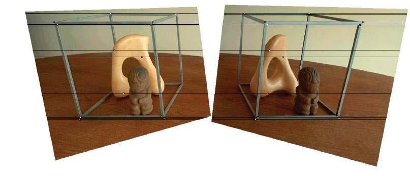
44 Stereo Vision versus Structure from Motion Stereo vision: is the process of obtaining depth information from a pair of images coming from two cameras that look at the same scene from different but known positions Structure from Motion: is the process of obtaining depth and motion information from a pair of images coming from the same camera that looks at the same scene from different positions 45

45 Depth from Stereo From a single camera, we can only deduct the ray on which each image point lies With a stereo camera (binocular), we can solve for the intersection of the rays and recover the 3D structure 3D Object Left Image Right Image Left Center of projection Right Center of projection

46 The human binocular system Stereopsys: the brain allows us to see the left and right retinal images as a single 3D image The images project on our retina up-side-down but our brains lets us perceive them as «straight». Radial disotion is also removed. This process is called «rectification»

47 The human binocular system Stereopsys: the brain allows us to see the left and right retinal images as a single 3D image The images project on our retina up-side-down but our brains lets us perceive them as «straight». Radial disotion is also removed. This process is called «rectification» Make a simple test: 1. Fix an object 2. Open and close alternatively the left and right eyes. The horizontal displacement is called disparity The smaller the disparity, the farther the object

48 The human binocular system Stereopsys: the brain allows us to see the left and right retinal images as a single 3D image The images project on our retina up-side-down but our brains lets us perceive them as «straight». Radial disotion is also removed. This process is called «rectification» disparity Make a simple test: 1. Fix an object 2. Open and close alternatively the left and right eyes. The horizontal displacement is called disparity The smaller the disparity, the farther the object

49 4c 40 Stereo Vision - The simplified case 4c - Perception - Vision The simplified case is an ideal case. It assumes that both cameras are identical and are aligned on a horizontal axis Z P ( X P, YP, ZP) f Z f Z From Similar Triangles: P P ul X P ur b X P Z P bf u u l r f C l u l b Baseline distance between the optical centers of the two cameras u r C r X Disparity difference in image location of the projection of a 3D point in two image planes R. Siegwart, D. Scaramuzza and M.Chli, ETH Zurich -

50 4c 41 Stereo Vision facts 4c - Perception - Vision Z P u l bf u r 1. Depth is inversely proportional to disparity Foreground objects have bigger disparity than background objects 2. Disparity is proportional to stereo-baseline b ( u u r) The smaller the baseline b the more uncertain our estimate of depth However, as b is increased, some objects may appear in one camera, but not in the other (remember both cameras have parallel optical axes) 3. The projections of a single 3D point onto the left and the right stereo images are called correspondence pair l R. Siegwart, D. Scaramuzza and M.Chli, ETH Zurich -

51 Choosing the Baseline What s the optimal baseline? Too small: Large depth error Can you quantify the error as a function of the disparity? Too large: Minimum measurable distance increases Difficult search problem for close objects Large Baseline Small Baseline

52 Stereo Vision general case Two identical cameras do not exist in nature! Aligning both cameras on a horizontal axis is very difficult In order to use a stereo camera, we need to know the intrinsic extrinsic parameters of each camera, that is, the relative pose between the cameras (rotation, translation) We can solve for this through camera calibration ( X w, Yw, Zw) 51

53 To estimate the 3D position of we can construct the system of equations of the left and right camera Triangulation is the problem of determining the 3D position of a point given a set of corresponding image locations and known camera poses. 52 Stereo Vision general case ),, ( w w w Z Y X T Z Y X R K v u p w w w r r r r r 1 ~ w w w l l l l l Z Y X K v u p 1 ~ Left camera: set the world frame to coincide with the left camera frame Right camera:

54 Correspondence Search the problem Goal: identify corresponding points in the left and right images, which are the reprojection of the same 3D scene point Typical similarity measures: Normalized Cross-Correlation (NCC), Sum of Squared Differences (SSD), Sum of Absolute Differences (SAD), Census Transform Exhaustive image search can be computationally very expensive! Can we make the correspondence search in 1D? 53

55 Similarity measures Sum of Squared Differences (SSD) Sum of Absolute Differences (SAD) (used in optical mice) k k u k k v v u F v u H SSD 2 ), ( ), ( k k u k k v v u F v u H SAD ), ( ), (

56 Similarity measures For slight invariance to intensity changes, the Zero-mean Normalized Cross Correlation (ZNCC) is widely used k k u k k v F k k u k k v H k k u k k v F H v u F v u H v u F v u H ZNCC 2 2 ), ( ), ( ), ( ), ( ), ( 1 2 ), ( N v u F N v u H k k u k k v F k k u k k v H

57 Correspondence Problem Exhaustive image search can be computationally very expensive! Can we make the correspondence search in 1D? Potential matches for have to lie on the corresponding epipolar line The epipolar line is the projection of the infinite ray corresponding to in the other camera image The epipole is the projection of the optical center in in the other camera image = = epipolar line C l = epipole C r

58 Correspondence Search the epipolar constraint The epipolar plane is defined by the image point and the optical centers Impose the epipolar constraint to aid matching: search for a correspondence along the epipolar line epipolar line epipolar plane epipolar line C l C r 55

59 Correspondence Search the epipolar constraint Thanks to the epipolar constraint, corresponding points can be searched for, along epipolar lines computational cost reduced to 1 dimension! 56

60 Example: horizontally aligned cameras Left image Right image

61 Stereo Rectification Even in commercial stereo cameras the left and right image are never perfectly aligned In practice, it is convenient if image scanlines are the epipolar lines Stereo rectification warps the left and right images into new rectified images, whose epipolar lines are aligned to the baseline

62 Stereo Rectification Reprojects image planes onto a common plane parallel to the baseline It works by computing two homographies (image warping), one for each input image reprojection As a result, the new epipolar lines are horizontal and the scanlines of the left and right image are aligned

63 Epipolar Rectification - Example First, remove radial distortion Left Right 62

64 Epipolar Rectification - Example First, remove radial distortion Then, compute homographies (warping) and rectify Left Right 63

65 Stereo Rectification: example

66 Stereo Vision disparity map The disparity map holds the disparity value at every pixel: Identify correspondent points of all image pixels in the original images Compute the disparity for each pair of correspondences Usually visualized in gray-scale images Close objects experience bigger disparity; thus, they appear brighter in disparity map Left image Right image Disparity Map 65

67 Stereo Vision disparity map The disparity map holds the disparity value at every pixel: Identify correspondent points of all image pixels in the original images Compute the disparity for each pair of correspondences Usually visualized in gray-scale images Close objects experience bigger disparity; thus, they appear brighter in disparity map From the disparity, we can compute the depth as: Z bf u l u r 66

68 Stereo Vision - summary 3D Object Left Image Right Image 1. Stereo camera calibration compute camera relative pose 2. Epipolar rectification align images & epipolar lines 3. Search for correspondences 4. Output: compute stereo triangulation or disparity map

69 Correspondence problem Now that the left and right images are rectified, the correspondence search can be done along the same scanlines

70 Correspondence problem If we look at the intensity profiles of two corresponding scanlines, there is a clear correspondence between intensities but also noise and ambiguities

71 Correlation-based window matching

72 Correspondence Problems: Textureless regions (the aperture problem) Textureless regions are non-distinct; high ambiguity for matches.

73 Solution: increase window size

74 Effects of window size W Smaller window + More detail More noise W = 3 W = 20 Larger window + Smoother disparity maps Less detail

75 Failures of correspondence search Textureless surfaces Occlusions, repetition

76 How can we improve window-based matching? Beyond the epipolar constraint, there are soft constraints to help identify corresponding points Uniqueness Only one match in right image for every point in left image Ordering Points on same surface will be in same order in both views Disparity gradient Disparity changes smoothly between points on the same surface Grauman

77 Results with window search Data Window-based matching Ground truth

78 Better methods exist... Graph cuts Ground truth Y. Boykov, O. Veksler, and R. Zabih, Fast Approximate Energy Minimization via Graph Cuts, PAMI 2001 For code, datasets, and comparisons all the algorithms:

79 Sparse correspondence search Restrict search to sparse set of detected features Rather than pixel values (or lists of pixel values) use feature descriptor and an associated similarity metrics Still use epipolar geometry to narrow the search further

80 Stereo Vision - summary 3D Object Left Image Right Image 1. Stereo camera calibration compute camera relative pose 2. Epipolar rectification align images & epipolar lines 3. Search for correspondences 4. Output: compute stereo triangulation or disparity map 5. Consider how baseline & image resolution affect accuracy of depth estimates

81 SFM: Structure From Motion (watch video segment) Given image point correspondences, x i x i /, determine R and T Keep track of point trajectories over multiple views to reconstruct scene structure and motion x x / C (R,T) C /