Moving Beyond Linearity

Transcription

1 Moving Beyond Linearity The truth is never linear! 1/23

2 Moving Beyond Linearity The truth is never linear! r almost never! 1/23

3 Moving Beyond Linearity The truth is never linear! r almost never! But often the linearity assumption is good enough. 1/23

4 Moving Beyond Linearity The truth is never linear! r almost never! But often the linearity assumption is good enough. When its not... polynomials, step functions, splines, local regression, and generalized additive models o er a lot of flexibility, without losing the ease and interpretability of linear models. 1/23

5 Polynomial Regression y i = x i + 2 x 2 i + 3 x 3 i d x d i + i Degree 4 Polynomial Wage Pr(Wage>250 Age) Age Age 2/23

6 Details Create new variables X 1 = X, X 2 = X 2, etc and then treat as multiple linear regression. 3/23

7 Details Create new variables X 1 = X, X 2 = X 2, etc and then treat as multiple linear regression. Not really interested in the coe cients; more interested in the fitted function values at any value x 0 : ˆf(x 0 )= ˆ0 + ˆ1x 0 + ˆ2x ˆ3x ˆ4x /23

8 Details Create new variables X 1 = X, X 2 = X 2, etc and then treat as multiple linear regression. Not really interested in the coe cients; more interested in the fitted function values at any value x 0 : ˆf(x 0 )= ˆ0 + ˆ1x 0 + ˆ2x ˆ3x ˆ4x 4 0. Since ˆf(x 0 ) is a linear function of the ˆ`, can get a simple expression for pointwise-variances Var[ ˆf(x 0 )] at any value x 0. In the figure we have computed the fit and pointwise standard errors on a grid of values for x 0.We show ˆf(x 0 ) ± 2 se[ ˆf(x 0 )]. 3/23

9 Details Create new variables X 1 = X, X 2 = X 2, etc and then treat as multiple linear regression. Not really interested in the coe cients; more interested in the fitted function values at any value x 0 : ˆf(x 0 )= ˆ0 + ˆ1x 0 + ˆ2x ˆ3x ˆ4x 4 0. Since ˆf(x 0 ) is a linear function of the ˆ`, can get a simple expression for pointwise-variances Var[ ˆf(x 0 )] at any value x 0. In the figure we have computed the fit and pointwise standard errors on a grid of values for x 0.We show ˆf(x 0 ) ± 2 se[ ˆf(x 0 )]. We either fix the degree d at some reasonably low value, else use cross-validation to choose d. 3/23

10 Details continued Logistic regression follows naturally. For example, in figure we model Pr(y i > 250x i )= exp( x i + 2 x 2 i dx d i ) 1 + exp( x i + 2 x 2 i dx d i ). To get confidence intervals, compute upper and lower bounds on on the logit scale, and then invert to get on probability scale. 4/23

11 Details continued Logistic regression follows naturally. For example, in figure we model Pr(y i > 250x i )= exp( x i + 2 x 2 i dx d i ) 1 + exp( x i + 2 x 2 i dx d i ). To get confidence intervals, compute upper and lower bounds on on the logit scale, and then invert to get on probability scale. Can do separately on several variables just stack the variables into one matrix, and separate out the pieces afterwards (see GAMs later). 4/23

12 Details continued Logistic regression follows naturally. For example, in figure we model Pr(y i > 250x i )= exp( x i + 2 x 2 i dx d i ) 1 + exp( x i + 2 x 2 i dx d i ). To get confidence intervals, compute upper and lower bounds on on the logit scale, and then invert to get on probability scale. Can do separately on several variables just stack the variables into one matrix, and separate out the pieces afterwards (see GAMs later). Caveat: polynomials have notorious tail behavior very bad for extrapolation. Can fit using y poly(x, degree = 3) in formula. 4/23

13 Bad tail behavior for polynomial regression Let us consider the function known as Runge s example (left panel) f(x) = 1 1+x 2 interpolated using a 15th polynomial(right panel). It turns out that high order interpolation using global polynomial often is dangerous.

14 Step Functions Another way of creating transformations of a variable cut the variable into distinct regions. C 1 (X) =I(X <35), C 2 (X) =I(35 apple X<50),...,C 3 (X) =I(X 65) Piecewise Constant Wage Pr(Wage>250 Age) Age Age 5/23

15 Step functions

16 Step functions Notice that for any value of X, C 0 (X) +C 1 (X) + + C K (X) = 1, since X must be in exactly one of the K +1intervals. We then use least squares to fit linear model using C 1 (X), C 2 (X),, C K (X) as predictors: y i = C 1 (X) + 1 C 1 (X) + + K C K (X) + i For logistic regression Pr(y i > 250x i ) = exp( C 1 (x i )) + + K C K (x i ) 1+exp( C 1 (x i )) + + K C K (x i )

17 Step functions continued Easy to work with. Creates a series of dummy variables representing each group. 6/23

18 Step functions continued Easy to work with. Creates a series of dummy variables representing each group. Useful way of creating interactions that are easy to interpret. For example, interaction e ect of Year and Age: I(Year < 2005) Age, I(Year 2005) Age would allow for di erent linear functions in each age category. 6/23

19 Step functions continued Easy to work with. Creates a series of dummy variables representing each group. Useful way of creating interactions that are easy to interpret. For example, interaction e ect of Year and Age: I(Year < 2005) Age, I(Year 2005) Age would allow for di erent linear functions in each age category. In R: I(year < 2005) or cut(age, c(18, 25, 40, 65, 90)). 6/23

20 Step functions continued Easy to work with. Creates a series of dummy variables representing each group. Useful way of creating interactions that are easy to interpret. For example, interaction e ect of Year and Age: I(Year < 2005) Age, I(Year 2005) Age would allow for di erent linear functions in each age category. In R: I(year < 2005) or cut(age, c(18, 25, 40, 65, 90)). Choice of cutpoints or knots can be problematic. For creating nonlinearities, smoother alternatives such as splines are available. 6/23

21 Basis functions Polynomial and piecewise-constant regression models are in fact special cases of a basis function approach. y i = b 1 (x i )+ 2 b 2 (x i )+ + K b K (x i )+ i where basis function b 1 ( ), b 2 ( ),, b K ( ) are fixed and known. For polynomial regression, b j (x i ) = x j i. For piecewise constant functions, b j (x i ) = I(c j apple x i < c j+1 ).

22 Moving Beyond Linearity

23 Piecewise Polynomials Instead of a single polynomial in X over its whole domain, we can rather use di erent polynomials in regions defined by knots. E.g. (see figure) ( x i + 21 x 2 i y i = + 31x 3 i + i if x i <c; x i + 22 x 2 i + 32x 3 i + i if x i c. Better to add constraints to the polynomials, e.g. continuity. Splines have the maximum amount of continuity. 7/23

24 Piecewise Cubic Continuous Piecewise Cubic Wage Wage Age Age Cubic Spline Linear Spline Wage Wage Age Age 8/23

25 Linear Splines A linear spline with knots at k,k=1,...,k is a piecewise linear polynomial continuous at each knot. We can represent this model as y i = b 1 (x i )+ 2 b 2 (x i )+ + K+3 b K+3 (x i )+ i, where the b k are basis functions. 9/23

26 Linear Splines A linear spline with knots at k,k=1,...,k is a piecewise linear polynomial continuous at each knot. We can represent this model as y i = b 1 (x i )+ 2 b 2 (x i )+ + K+3 b K+3 (x i )+ i, where the b k are basis functions. b 1 (x i ) = x i b k+1 (x i ) = (x i k ) +, k =1,...,K Here the () + means positive part; i.e. xi (x i k ) + = k if x i > k 0 otherwise 9/23

27 f(x) x b(x) x 10 / 23

28 Cubic Splines A cubic spline with knots at k,k=1,...,k is a piecewise cubic polynomial with continuous derivatives up to order 2 at each knot. Again we can represent this model with truncated power basis functions y i = b 1 (x i )+ 2 b 2 (x i )+ + K+3 b K+3 (x i )+ i, b 1 (x i ) = x i b 2 (x i ) = x 2 i b 3 (x i ) = x 3 i b k+3 (x i ) = (x i k ) 3 +, k =1,...,K where (x i k ) 3 + = (xi k ) 3 if x i > k 0 otherwise 11 / 23

29 f(x) x b(x) x 12 / 23

30 More for spline Simple linear model: y i = x i + i X matrix: quadratic model (polynomial) : X matrix: y i = x i + 2 x 2 i + i

31 More for spline

32 More for spline broken stick model: y i = x i + 11 (x i 0.6) + + i whip model (polynomial) : y i = x i + 11 (x i 0.5) (x i 0.55) + + 1k (x i 0.95) + + i X matrix: Spline model for f KX f (x) = x + b k (x k k ) + k=1

33 Splines Figure 6: *

34 Linear splines

35 cubic splines

36 cubic splines

37 B-Splines

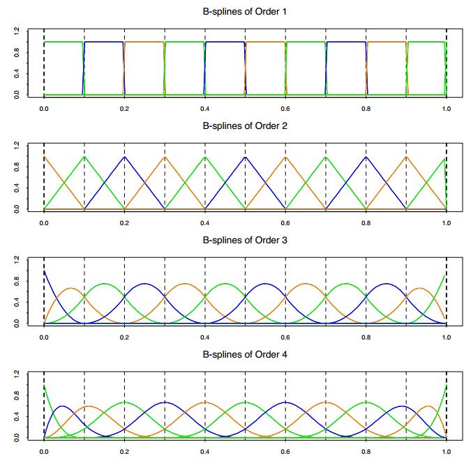
38 B-Splines

39 Natural cubic spline X consisting of 50 points drawn at random from U[0,1], and an assumed error model with constant variance. The linear and cubic polynomial fits have two and four degrees of freedom, respectively, while the cubic spline and natural cubic spline each have six degrees of freedom. The cubic spline has two knots at 0.33 and 0.66, while the natural spline has boundary knots at 0.1 and 0.9, and four interior knots uniformly spaced between them.

40 Natural Cubic Splines A natural cubic spline extrapolates linearly beyond the boundary knots. This adds 4 = 2 2 extra constraints, and allows us to put more internal knots for the same degrees of freedom as a regular cubic spline. Wage Natural Cubic Spline Cubic Spline / 23

41 Fitting splines in R is easy: bs(x,...) for any degree splines, and ns(x,...) for natural cubic splines, in package splines. Natural Cubic Spline Wage Pr(Wage>250 Age) Age Age 14 / 23

42 Knot placement ne strategy is to decide K, the number of knots, and then place them at appropriate quantiles of the observed X. A cubic spline with K knots has K + 4 parameters or degrees of freedom. A natural spline with K knots has K degrees of freedom. Wage Natural Cubic Spline Comparison of a Polynomial degree-14 polynomial and a natural cubic spline, each with 15df Age 15 / 23

43 Knot placement ne strategy is to decide K, the number of knots, and then place them at appropriate quantiles of the observed X. A cubic spline with K knots has K + 4 parameters or degrees of freedom. A natural spline with K knots has K degrees of freedom. Wage Natural Cubic Spline Comparison of a Polynomial degree-14 polynomial and a natural cubic spline, each with 15df. ns(age, df=14) poly(age, deg=14) Age 15 / 23

44 Smoothing spline In the last section, we create splines by specifying a set of knots, producing a sequence of basis funcitons and then using LS to estimate spline coefficients. Now, we introduce a somewhat different approach smoothing spline. In fitting a smooth curve to a set of data, we need to find function g(x) to fits the observed data well. That is we want RSS = P n i=1 (y i g(x i )) 2 to be small. However, if we don t put any constraints on g(x i ), then we can make RSS zero by choosing g such that it interpolates all of y i. verfit, too rough. How might we ensure that g is smooth?

45 Smoothing Splines This section is a little bit mathematical Consider this criterion for fitting a smooth function g(x) to some data: nx Z minimize (y i g(x i )) 2 + g 00 (t) 2 dt g2s i=1 16 / 23

46 Smoothing Splines This section is a little bit mathematical Consider this criterion for fitting a smooth function g(x) to some data: nx Z minimize (y i g(x i )) 2 + g 00 (t) 2 dt g2s i=1 The first term is RSS, and tries to make g(x) match the data at each x i. 16 / 23

47 Smoothing Splines This section is a little bit mathematical Consider this criterion for fitting a smooth function g(x) to some data: nx Z minimize (y i g(x i )) 2 + g 00 (t) 2 dt g2s i=1 The first term is RSS, and tries to make g(x) match the data at each x i. The second term is a roughness penalty and controls how wiggly g(x) is. It is modulated by the tuning parameter / 23

48 Smoothing Splines This section is a little bit mathematical Consider this criterion for fitting a smooth function g(x) to some data: nx Z minimize (y i g(x i )) 2 + g 00 (t) 2 dt g2s i=1 The first term is RSS, and tries to make g(x) match the data at each x i. The second term is a roughness penalty and controls how wiggly g(x) is. It is modulated by the tuning parameter 0. The smaller, the more wiggly the function, eventually interpolating y i when = / 23

49 Smoothing Splines This section is a little bit mathematical Consider this criterion for fitting a smooth function g(x) to some data: nx Z minimize (y i g(x i )) 2 + g 00 (t) 2 dt g2s i=1 The first term is RSS, and tries to make g(x) match the data at each x i. The second term is a roughness penalty and controls how wiggly g(x) is. It is modulated by the tuning parameter 0. The smaller, the more wiggly the function, eventually interpolating y i when = 0. As!1, the function g(x) becomes linear. 16 / 23

50 Smoothing Splines continued The solution is a natural cubic spline, with a knot at every unique value of x i. The roughness penalty still controls the roughness via. 17 / 23

51 Smoothing Splines continued The solution is a natural cubic spline, with a knot at every unique value of x i. The roughness penalty still controls the roughness via. Some details Smoothing splines avoid the knot-selection issue, leaving a single to be chosen. 17 / 23

52 Smoothing Splines continued The solution is a natural cubic spline, with a knot at every unique value of x i. The roughness penalty still controls the roughness via. Some details Smoothing splines avoid the knot-selection issue, leaving a single to be chosen. The algorithmic details are too complex to describe here. In R, the function smooth.spline() will fit a smoothing spline. 17 / 23

53 Smoothing Splines continued The solution is a natural cubic spline, with a knot at every unique value of x i. The roughness penalty still controls the roughness via. Some details Smoothing splines avoid the knot-selection issue, leaving a single to be chosen. The algorithmic details are too complex to describe here. In R, the function smooth.spline() will fit a smoothing spline. The vector of n fitted values can be written as ĝ = S y, where S is a n n matrix (determined by the x i and ). The e ective degrees of freedom are given by df = nx {S } ii. i=1 17 / 23

54 Smoothing spline It can be shown the criterion of smoothing spline has an explicit, finite-dimensional, unique minimizer which is a natrural cubic spline with knots at the unique values of the x i, i = 1,, N. We can write f (x) as f (x) = NX N j (x) j i=1, where the N j (x) are an N dimensional set of basis functions. The criterion thus reduces to

55 Smoothing spline

56 Smoothing spline

57 Smoothing spline

58 Smoothing spline

59 Smoothing spline Reinsch form ŷ = N (N T N + N ) 1 N T y = N (N T [I + N T N 1 ]N) 1 N T y K is known as the penalty matrix. = (I + N T N 1 ) 1 y = (I + K) 1 y (6)

60 Smoothing spline The eigen decomposition of S and d k the corresponding eigenvalue of K.

61 Smoothing spline

62 Smoothing spline

63 Smoothing Splines continued choosing We can specify df rather than! In R: smooth.spline(age, wage, df = 10) 18 / 23

64 Smoothing Splines continued choosing We can specify df rather than! In R: smooth.spline(age, wage, df = 10) The leave-one-out (L) cross-validated error is given by RSS cv ( )= nx (y i ĝ ( i) (x i )) 2 = i=1 nx apple yi ĝ (x i ) i=1 1 {S } ii 2. In R: smooth.spline(age, wage) 18 / 23

65 Smoothing Spline Wage Degrees of Freedom 6.8 Degrees of Freedom (LCV) Age 19 / 23

66 Local Regression Local Regression With a sliding weight function, we fit separate linear fits over the range of X by weighted least squares. See text for more details, and loess() function in R. 20 / 23

67 local regression

68 local regression locally weighted regression solves a separate weighted least squares prob- lem at each target point x 0 : the estimate is then f ˆ(x 0 ) = (x ˆ 0 )+ (x ˆ 0 )x 0 define the vector function b(x) T = (1, x), let B be the N 2 rgression matrix with ith row b(x i ) T, and W (x 0 ) the N N diagonal matrix with ith diagonal element K (x 0, x i ), then

69 Multidimensional spline

70 Multidimensional spline

71 Generalized Additive Models Allows for flexible nonlinearities in several variables, but retains the additive structure of linear models. y i = 0 + f 1 (x i1 )+f 2 (x i2 )+ + f p (x ip )+ i. <HS HS <Coll Coll >Coll f1(year) f2(age) f3(education) year age education 21 / 23

72 Fitting a GAM I If the functions f 1 have a basis representation, we can simply use least squares: I I I Natural cubic splines Polynomials Step functions wage = 0 + f 1 (year)+f 2 (age)+f 3 (education)+ 17 / 24

73 Fitting a GAM I therwise, we can use backfitting: 18 / 24

74 Fitting a GAM I therwise, we can use backfitting: 1. Keep f 2,...,f p fixed, and fit f 1 using the partial residuals: y i 0 f 2 (x i2 ) f p (x ip ), as the response. 18 / 24

75 Fitting a GAM I therwise, we can use backfitting: 1. Keep f 2,...,f p fixed, and fit f 1 using the partial residuals: y i 0 f 2 (x i2 ) f p (x ip ), as the response. 2. Keep f 1,f 3,...,f p fixed, and fit f 2 using the partial residuals: y i 0 f 1 (x i1 ) f 3 (x i3 ) f p (x ip ), as the response. 18 / 24

76 Fitting a GAM I therwise, we can use backfitting: 1. Keep f 2,...,f p fixed, and fit f 1 using the partial residuals: y i 0 f 2 (x i2 ) f p (x ip ), as the response. 2. Keep f 1,f 3,...,f p fixed, and fit f 2 using the partial residuals: y i 0 f 1 (x i1 ) f 3 (x i3 ) f p (x ip ), as the response / 24

77 Fitting a GAM I therwise, we can use backfitting: 1. Keep f 2,...,f p fixed, and fit f 1 using the partial residuals: y i 0 f 2 (x i2 ) f p (x ip ), as the response. 2. Keep f 1,f 3,...,f p fixed, and fit f 2 using the partial residuals: y i 0 f 1 (x i1 ) f 3 (x i3 ) f p (x ip ), as the response Iterate 18 / 24

78 Fitting a GAM I therwise, we can use backfitting: 1. Keep f 2,...,f p fixed, and fit f 1 using the partial residuals: y i 0 f 2 (x i2 ) f p (x ip ), as the response. 2. Keep f 1,f 3,...,f p fixed, and fit f 2 using the partial residuals: y i 0 f 1 (x i1 ) f 3 (x i3 ) f p (x ip ), as the response Iterate I This works for smoothing splines and local regression. 18 / 24

79 GAM details Can fit a GAM simply using, e.g. natural splines: lm(wage ns(year, df = 5)+ ns(age, df = 5)+ education) 22 / 23

80 GAM details Can fit a GAM simply using, e.g. natural splines: lm(wage ns(year, df = 5)+ ns(age, df = 5)+ education) Coe cients not that interesting; fitted functions are. The previous plot was produced using plot.gam. 22 / 23

81 GAM details Can fit a GAM simply using, e.g. natural splines: lm(wage ns(year, df = 5)+ ns(age, df = 5)+ education) Coe cients not that interesting; fitted functions are. The previous plot was produced using plot.gam. Can mix terms some linear, some nonlinear and use anova() to compare models. 22 / 23

82 GAM details Can fit a GAM simply using, e.g. natural splines: lm(wage ns(year, df = 5)+ ns(age, df = 5)+ education) Coe cients not that interesting; fitted functions are. The previous plot was produced using plot.gam. Can mix terms some linear, some nonlinear and use anova() to compare models. Can use smoothing splines or local regression as well: gam(wage s(year, df = 5)+ lo(age, span =.5)+ education) 22 / 23

83 GAM details Can fit a GAM simply using, e.g. natural splines: lm(wage ns(year, df = 5)+ ns(age, df = 5)+ education) Coe cients not that interesting; fitted functions are. The previous plot was produced using plot.gam. Can mix terms some linear, some nonlinear and use anova() to compare models. Can use smoothing splines or local regression as well: gam(wage s(year, df = 5)+ lo(age, span =.5)+ education) GAMs are additive, although low-order interactions can be included in a natural way using, e.g. bivariate smoothers or interactions of the form ns(age,df=5):ns(year,df=5). 22 / 23

84 p(x) log 1 p(x) GAMs for classification = 0 + f 1 (X 1 )+f 2 (X 2 )+ + f p (X p ). HS <Coll Coll >Coll f1(year) f2(age) f3(education) year age education gam(i(wage > 250) year + s(age, df = 5)+education, family = binomial) 23 / 23

85 GAM

86 Nonparametric Beta regression Fractional data that are restricted in the standard unit interval (0, 1) with a highly skewed distribution are commonly encountered. the linear regression model cannot always guarantee that the fitted or predicted values will fall into the unit interval (0, 1). To overcome such issues, one possible approach is to first transform the response such that it can take values within ( 1, +1) and then apply a regression model to the transformed response. such an approach still has shortcomings; one shortcoming is that the coefficients cannot easily be interpreted in terms of the original response, and another shortcoming is that the fractional response is generally asymmetric and highly skewed. one appealing model is beta regression, which response variable is assumed to follow a beta distribution within the unit interval (0,1).

87 Nonparametric Beta regression Let (y i, X > i )>, i = 1,...,n, be vectors that are independent and identically distributed as (y, X), where y is a response variable that is restricted to the unit interval (0,1) and X i = (x i1,, x ip ) > 2 R p is the ith observation of the p covariates, which are assumed to be fixed and known. The beta density is: f (y; µ, ) = ( ) (µ ) ( ) yµ 1 (1 y) (1 µ) 1, (1) where µ 2 (0, 1) is the mean of y, > 0 is a precision parameter, and ( ) is the gamma function. The variance of y is var(y) = µ(1 µ)/(1 + ). linear beta regression model: g(µ i ) = px x ij j, (2) where g( ) is a strictly monotonic and twice-differentiable link function that maps (0,1) into R; j=1

88 Nonparametric Beta regression we propose nonparametric additive beta regression: px g(µ i ) = f j (x ij ), (3) j=1 where µ i = E(y i ), i = 1,, n. g( ) is a strictly monotonic and twice- differentiable link function that maps (0, 1) into R, and we use the logit link function g(µ) = log µ/(1 µ) in this study. f j s are unknown smooth functions to be estimated, and suppose that some of them are zero. using B-splines to approximate each of the unknown functions f j s, we can have the following approximation f j (x) t f nj (x) = Xm n k=1 jk k (x) with m n coefficients jk, k = 1,, m n. px Xm n g(µ i ) t 0 + jk k (x ij ). (4) j=1 k=1

89 Nonparametric Beta regression The objective function: L(, ) = l(, ) n px w j (m n )P ( j 2 ), (5) where l(, ) = P n i=1 l i (µ i, ) is the log-likelihood function; l i (µ i, ) = ln ( ) ln (µ i ) ln ((1 µ i ) ) + (µ i 1) ln y i + {(1 µ i ) 1} ln(1 y i ); P ( ) is a penalty function, w j ( ) is used to rescale the penalty with respect to the dimensionality of the parameter vector j. The penalized likelihood estimators are then defined as ( n, ) = argmax, L(, ). j=1

90 Nonparametric Beta regression Theorem (Estimation consistency). Define F T = { j : nj 2, 0, 1 apple j apple p}, and let M denote the cardinality of any set M {1,, p}. Under conditions (C1) (C4), we can obtain the following: (i) With probability converging to 1, F T apple M 1 F T = M 1 q for a finite constant M 1 > 1. (ii) If max{p 0 ( j 2 )} 2 m n /n 2! 0 as n!1, then P( F T F T )! p 1. pp (iii) nj j 2 2 = p(mn 2d+1 ) + p ( 4 max {P0 ( j 2 ) } 2 m 2 n ). n 2 j=1

91 Theorem (Selection consistency). Under conditions (C1) (C5), we have: (i) P( n= 0 )! 1. Define fˆ j (x) = m Pn have k=1 jk k (x). Under conditions (C1) (C5), we (i) P( ˆf j 2 > 0, j 2 F T and ˆf j 2 = 0, j 2 F F /F T )! p 1. qp (ii) fˆ j f j 2 2 = p mn 2d + p 4m n (max {P 0 ( j 2 )}) 2 /n 2. j=1