Chapter 3. Illumination Models and Surface-Rendering Methods. Department of Computer Science and Engineering

Transcription

1 Chapter 3 Illumination Models and Surface-Rendering Methods 3-1

2 3.1 Overview For a realistic display of a scene the lighting effects should appear naturally. An illumination model, also called a lighting model, is used to compute the color of an illuminated position on the surface of an object. The shader model then determines when this color information is computed by applying the illumination model to identify the pixel colors for all projected positions in the scene. Different approaches are available that calculate the color for each pixel individually or interpolate between pixels in the vicinity. This chapter will introduce the basic concepts that are necessary for achieving different lighting effects. 3-2

3 3.1 Overview Using correct lighting improves the three-dimensional impression. 3-3

4 3.1 Overview In particular, this chapter covers the following: Light sources Shading models Polygon rendering methods Ray-tracing methods Radiosity lighting model Texture mapping OpenGL illumination and surface-rendering OpenGL texture functions 3-4

5 3.2 Light Sources Often in computer graphics, light sources are assumed as simple points. This is basically due to the fact that it is easier to do all the necessary lighting computations with point light sources. Diverging ray paths from a point light source 3-5

6 3.2 Light Sources Radial intensity attenuation As the radial intensity from a light source travels outwards its amplitude at any distance d l from the source is attenuated quadratically: f RadAtten ( d l ) = a a d + 1 l a 2 d 2 l For light sources, that are located very far away from the objects of the scene it is safe to assume that there is no attenuation, i.e. f RadAtten =

7 3.2 Light Sources Directional light sources By limited the direction of the light source, directional light sources, or spotlights, can be created. Then, only objects that divert at a maximal angle θ l are lit by the light source. light direction vector L (normalized) θ l 3-7

8 3.2 Light Sources Directional light sources (continued) To determine if an object is lit by the light source, we need to compare the angle between the light direction vector and the vector to the object, e.g. its vertices. L α object θ l V o Assuming that 0<θ l 90º we can check if an object is lit by comparing the angles: cos α = L V o cos θ l 3-8

9 3.2 Light Sources Directional light sources (continued) In analogy to radial attenuation, we can introduce an attenuating effect for spotlights as well based on the angle: 1.0 if source is not a spotlight f AngAtten = 0.0 object is outside the spotlight (L V o ) a l otherwise 3-9

10 3.2 Shading model Illumination model For determining the intensity (color) of a pixel, which results from the projection of an object (for example a polygon), illumination models are used. An illumination model describes how to compute a intensity (color) of a point within the scene depending on the incoming light from different light sources. The computation is usually done in object space. In many illumination models, the intensity (color) of a point depends on the incoming direct light from light sources and indirect light approximating reflection of light from surrounding objects. 3-10

11 3.2 Shading model Shading model Two different approaches for applying the illumination model are possible to determine all pixels of the resulting image. The illumination model can be applied to Each projected position individually Certain projected position; the pixels in between are then interpolated interpolating shading techniques, e.g. flat shading, Gouraud shading, or Phong shading 3-11

12 3.2 Shading model Interpolating shading techniques world coordinates screen coordinates illumination model: The intensity of a point on a surface of an object is computed interpolating shading algorithm: Interpolates pixel intensities by interpolating intensities of poylgon vertices 3-12

13 3.2 Shading model Interpolating shading techniques (continued) world Does this state a problem? coordinates Lighting of the scene is done in object space (world coordinates Interpolation of intensity values is done in image space Projections generally are not affine transformations By using an interpolating scheme (e.g. linear interpolation) we use incorrect ratios with respect to the world coordinate system Despite being mathematically incorrect, this shading model achieves fast and acceptable results screen coordinates 3-13

14 3.2 Shading model Geometry theta phi P P point on the object s surface N surface normal vector at P, normalized L vector pointing from P towards a point light source, normalized V vector pointing from P towards the view point (eye), normalized φ i, θ I (local) spherical coordinates (of L and V) 3-14

15 3.2 Shading model Specular Reflection R vector of the reflected ray, normalized N L R θ θ R 2 We obtain: L and R are located in the same R = = R 2 + R 1 R 1 2R 2 L Plane and θ = θ in = θ ref = 2( L N) N L 3-15

16 3.2 Shading model We first consider the most common illumination model: the Phong illumination model. Careful: this model is based on empirical results without any physical meaning but with good and practical results! The model simulates the following physical reflective properties: a) Perfect/full specular reflection A light ray is completely reflected without any scattering according to the laws of reflection. Surface: ideal mirror (does not exist in reality) 3-16

17 3.2 Shading model Simulated physical reflective properties (continued) b) Partly specular reflection The light ray is split up so that a reflective conus occurs with the full specular reflection as its main extent. Surface: imperfect mirror, rough surface; a surface element is composed of microscopically small ideal mirrors which are leveled slightly differently. 3-17

18 3.2 Shading model Simulated physical reflective properties (continued) c) Perfect/full diffuse reflection The light ray is perfectly scattered, i.e. with the same intensity in all direction Surface: ideal, matt surface (does not exist in reality); approximates e.g. fine layer of powder The Phong illumination model then composes the reflected light linearly out of these three components: reflected light = diffuse component + specular component + ambient light 3-18

19 3.2 Shading model 3-19

20 3.2 Shading model Ambient light The ambient component is usually defined as constant and simulates the global and indirect lighting. This is necessary because some objects are not hit by any light rays and would end up as being black. In reality, these objects would be lit by indirect light reflected by surrounding objects. Hence, ambient light is just a mean to cope for the missing indirect lighting. What kind of surfaces can be simulated with this model? The linear combination of different components (diffuse and specular) resemble, for example, polished surfaces. 3-20

21 3.2 Shading model Polished surfaces 3-21

22 3.2 Shading model The mathematical model (without color information) I = k d I d + k s I s + k a I a The physical properties of the surface are determined by the ratios between the different components. The constants always add up to one: k d + k s + k a = 1 Diffuse reflection, i.e. the term k d I d I d = I i cos (θ) with I i intensity of the incoming light θ angle between normal N and light vector L 3-22

23 3.2 Shading model Diffuse reflection (continued) I d = I i (L N) The diffuse component of the Phong model emulates Lambert s cosine law: Ideal diffuse (matt) surfaces reflect the light at an intensity (in all directions equally) identical to the cosine between surface normal and light vector 3-23

24 3.2 Shading model Specular reflection From a physical point of view, the specular reflection forms an image of the light source smeared across the surface. This is usually called a highlight. A highlight can only be seen by the viewer if her/his viewing direction V is close to the direction of the reflection R. This can be simulated by: I s = I i cos n (Ω) with Ω angle between V and R n simulates degree of perfection of the surface (n simulates a perfect mirror, i.e. only reflects in direction of R) 3-24

25 3.2 Shading model Specular reflection (continued) I s = I i (R V) n Comments: For different L we always get (except its direction R) the same reflection cone. This does not concur with the real relation between reflection and direction of the light vector. Major drawback of this model! 3-25

26 3.2 Shading model Entire mathematical model in detail: I = k d I d + k s I s + k a I a = I i (k d (L N) + k s (R V) n )+ k a I a As a 2-D section: specular diffuse ambient 3-26

27 3.2 Shading model Example: k a,k d constant increasing k s increasing n 3-27

28 3.2 Shading model Comment: If the view point is sufficiently, e.g. infinitely, far away from the light source we can replace the reflection vector R by a constant vector H: H = (L+V)/ L+V. Then we can use N H instead of R V, which differs from R V but has similar properties. Hence, we get: I = I i (k d (L N) + k s (N H) n )+ k a I a 3-28

29 3.2 Shading model The mathematical model: (including color) I r = I i (k dr (L N) + k sr (N H) n )+ k ar I a I g = I i (k dg (L N) + k sg (N H) n )+ k ag I a I b = I i (k db (L N) + k sb (N H) n )+ k ab I a where k dr,k dg,k db model the color of the object k sr,k sg,k sb model the color of the light source k ar,k ag,k ab (for white light: k sr, =k sg, =k sb model the color of the background light 3-29

30 3.2 Shading model Comments: Main deficiencies of the model: Two-way reflections and mirroring of surfaces are described insufficiently by the ambient term Surfaces appear like plastic, for example, metal cannot be modeled exactly physically based shading models, that try to simulate the BRDFs (reflection function, see next slide) correctly 3-30

31 3.2 Shading model BRDF (bi-directional reflection distribution function): In general, the reflected light emitted from a point on a surface can be described by a BRDF. The name BRDF specifically stresses the dependence of the light reflected in an arbitrary direction on the direction of the incoming light. If all directions L and V are known, the correlation between intensities are described by a BRDF: f(θ in,φ in,θ ref,φ ref ) = f(l,v) 3-31

32 3.2 Shading model BRDF (continued) In practice, incoming light enters from more than one direction at a specific point on the surface. The entire reflected light then has to be computed by integrating across the hemisphere to cover for all possible directions of incoming light. Questions: How to determine BRDFs? e.g. measuring, modeling What resolution is necessary to represent BRDFs? heuristics if there are no closed form representations How can BRDFs be stored and processed efficiently? e.g. matrices 3-32

33 3.2 Shading model BRDF (continued) Representation of BRDFs for two different directions of incoming light (modeled after Blinn (1977): 3-33

34 3.2 Shading model Disadvantages of entirely local shading models: Represent ideal case of a single object in a scene that is lit by a single point light source Only consider direct lighting Interaction with other objects is not modeled (i.e. no indirect lighting, no shadows) global shading techniques 3-34

35 3.3 Polygon rendering methods How can the evaluation of a specific illumination model for an object be used to determine the light intensities of the points on the object s surface? we assume a polygonal object representation consisting of several faces world coordinates Weltkoordinaten image Bildschirmkoordinaten coordinates There is a difference between (threedimensional) object space and (twodimensional) image space! 3-35

36 3.3 Polygon rendering methods Flat shading For each polygon/face, the illumination model is applied exactly once for a designated point on the surface. The resulting intensity is then used for all other points on that surface. The illumination model requires a polygon normal or surface normal in object space. (for example N 1, N 2, N 3, N 4, ) As designated point, often the center of gravity or, for simplicity reasons, one of the vertices is used. 3-36

37 3.3 Polygon rendering methods Flat shading (continued) Comments: Simple, cost-effective method; interpolation is not necessary Edges within polygonal networks remain visible, i.e. faces are visible; non-continuous intensity distribution across edges Can be used for pre-views, sketches, visualization of the polygonal resolution. 3-37

38 3.3 Polygon rendering methods Gouraud and Phong shading Both methods use interpolation techniques in order to smooth out or eliminate the visibility of the (virtual) edges. (the polygonal network represents an approximation of a curved surface) For the illumination model, the normal vectors at the shared vertices of the polygons are used (e.g. N A, ) A vertex normal can be derived from the (weighted) average of the normal vectors of the attached polygons or determined from the object originally represented by the polygonal network. 3-38

39 3.3 Polygon rendering methods Gouraud and Phong shading (continued) Both methods use (bi-)linear interpolation in the image space: Values inside (and on the edge of) a polygon are computed from the values at the vertices (generally determined in object space) by using linear P a (x a,y s ) interpolation within the image space. Efficient implementation work incrementally following the scan line. P 2 (x 2,y 2 ) P s (x s,y s ) P 1 (x 1,y 1 ) P 3 (x 3,y 3 ) P b (x b,y s ) P 4 (x 4,y 4 ) 3-39

40 3.3 Polygon rendering methods Gouraud and Phong shading (continued) 1. Determine values V(P 1 ), V(P 2 ), V(P 3 ), V(P 4 ) 2. Determine the intersections P a, P b between scan-line and edges of the polygon P a (x a,y s ) 3. Determine V(P a ) and V(P b ): V ( P V ( P 4. Determine V(P s ): V ( P ) = s a b ) = y ) = x y b y 1 y 1 x a 1 1 ( V ( P )( y y ) + V ( P )( y y )) ( V ( P )( y y ) + V ( P )( y y )) ( V ( P )( x x ) + V ( P )( x x )) a 1 1 b 2 4 s s s 4 b 2 s s s 1 1 a P 2 (x 2,y 2 ) P s (x s,y s ) P 1 (x 1,y 1 ) P 3 (x 3,y 3 ) P b (x b,y s ) P 4 (x 4,y 4 ) 3-40

41 3.3 Polygon rendering methods Gouraud shading The illumination model is only used for evaluating the intensities at the vertices of the polygons using the normal vectors of those vertices. Using interpolation, the intensity values at the (projected) points inside the polygon are computed. 3-41

42 3.3 Polygon rendering methods Gouraud shading (continued) Edges of the polygonal network are smoothed and the intensity distribution across the edge is continuous, however not necessarily smooth. Method cannot generate highlights appropriately: these can only occur if the view vector is very close to the direction of reflection; however, the illumination model is only evaluated at the vertices and hence may miss the highlights 3-42

43 3.3 Polygon rendering methods Gouraud shading (continued) Highlights are either skipped or appear shaped like a polygon (instead of round) Often used: combination of Gouraud shading and exclusively diffuse reflective component Comment: Gouraud shading is one of the standard shading methods used by today s graphics hardware 3-43

44 3.3 Polygon rendering methods Phong shading The illumination model is evaluated for every projected point of the polygonal surface. The surface normal at each projected point is computed by interpolating the normals at the vertices. 3-44

45 3.3 Polygon rendering methods Phong shading Intensity distribution across the edges of the polygon network is continuous and smooth; the appearance of curved surfaces is approximated very well using the interpolated normal vectors Much more computational effort required compared to Gouraud shading. Highlights are represented adequately. Comment: Phong shading is supported by current high-end graphics hardware. 3-45

46 3.3 Polygon rendering methods Flat, Gouraud and Phong shading in comparison 3-46

47 3.3 Polygon rendering methods Comments: What do we need to do to ensure that polygon edges that are explicitly supposed to appear as edges when using Gouraud or Phong shading? Vertices of the polygon that are part of such feature edges have to be stored separately and with different normal vectors. Strong connection and dependence between shading method and polygonization or triangulation of the object (feature recognition) 3-47

48 3.3 Polygon rendering methods Before the perceived images are transmitted to the brain, the cells in the human eye pre-process the intensity values. How do the light receptors in the eye react to different light intensities? Lechner s law The relation between the light entering the eye and the light intensity perceived by the eye is not linear but approximately logarithmic. 3-48

49 3.3 Polygon rendering methods Lechner s law (continued) Implication: Small changes to the intensity in dark areas are perceived better than the exact same change in intensity in brighter areas. 3-49

50 3.3 Polygon rendering methods Lechner s law (continued) Intensity progression / color progression Intensity increase of equidistant steps of 12.5% with respect to incoming light (0% to 100% Jump in intensities in darker areas appears significantly larger than in lighter areas Great difference between perceived jumps in intensities Increase in intensities in equidistant steps with respect to perceived intensities Perception of almost equidistant jumps in intensity 3-50

51 3.3 Polygon rendering methods Mach band effect The interaction of the light receptors in the human eye emphasize sharp changes in intensity. As soon as the eye detects such changes in incoming intensity, it adds overshoot and undershoot to the received intensity which amplify the difference. This sub-conscious mechanism of highlighting edges between different intensities helps our visual perception to automatically sharpen contours (edge detection). 3-51

52 3.3 Polygon rendering methods Mach band effect (continued) Example: 3-52

53 3.3 Polygon rendering methods Mach band effect (continued) When rendering, the automatic detection of changes in intensity of the human eye is rather disturbing and can only be reduced by generating transitions between different intensities as smooth as possible. Flat shading: non-continuous transitions in intensity, very strong Mach band effect Gouraud shading: continuous change in intensity; nevertheless still Mach band effects depending on the polyonization Phong shading: smooth transition between intensities reduce Mach band effect significantly 3-53

54 3.3 Polygon rendering methods Mach band effect (continued) Mach band effect occurring when using Gouraud shading 3-54

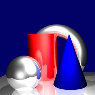
55 3.4 Ray-tracing Principle Backward ray-tracing: since most light rays do not hit the eye it requires less computational effort to trace the light rays backwards starting at the eye and then end at the individual light sources and other surfaces. The rays are traced for every pixel within the image place into the scene; at every intersection with an object, the direct (local model) as well as the reflected and refracted light components are determined. The resulting bifurcations of the rays implicitly describe a tree. Ray-tracing is specifically suitable for modeling of directed light (many mirror-like or transparent objects) 3-55

56 3.4 Ray-tracing Opaque Object Light Light Rays / Shadow Rays Initial Ray Eye Pixel Semi-transparent object 3-56

57 3.4 Ray-tracing Recursively tracing of rays 3-57

58 3.4 Ray-tracing Recursively tracing rays (continued) Refraction occurs at the common boundary between media with different densities, e.g. air and water. The angle of refraction β is proportional to the angle of incidence β. If the ray enters a more dense medium the angle is going to decrease. Surfaces can (partly) reflect and refract at the same time. However, if the angle of refraction β is greater than 90 the ray is only reflected. 3-58

59 3.4 Ray-tracing Examples: 3-59

60 3.4 Ray-tracing Recursively tracing rays (continued) The ray is terminated if The reflected or refracted ray does not intersect any more objects. A maximal depth of the tree is reached. The contribution in intensity (color) value of a continued ray becomes too low. Comment: The computational effort of this approach depends heavily on the complexity of the scene. Space subdivision techniques, such as octrees, can result in significant speed-ups when using ray-tracing. 3-60

61 3.4 Ray-tracing Shadows Follow a ray from every intersection with an object to all light sources. If one of those rays has to pass through an object on its way to the light source then the point of intersection is not lit by this light source, hence it is in its shadow. 3-61

62 3.4 Ray-tracing Shadows (continued) 3-62

63 3.4 Ray-tracing Distributed ray-tracing In reality, there is no perfect mirror, since no mirror is absolutely planar and reflects purely (100%). Distributed ray-tracing allows the generation of realistic blur effects for ray-tracing. Instead of using a single reflected ray several rays are traced and the resulting intensities averaged. 3-63

64 3.4 Ray-tracing Distributed ray-tracing (continued) Most of those rays follow more or less the reflected direction while a few brake with this behavior resulting in a bulb-shaped distribution. 3-64

65 3.4 Ray-tracing Distributed ray-tracing (continued) Similarly, a refracted ray is spread out using the same pattern. Using a stochastic distribution across all possible directions of reflection and refraction and then averaging, we get a realistic approximation. 3-65

66 3.4 Ray-tracing Distributed ray-tracing larger light sources An additional increase in realism can be achieved by allowing light sources not to be just point-shaped. A larger light emitting surface area can be modeled, for example, by using numerous point-shaped light sources. By deploying suitable stochastic distributions of rays, realistic soft-shadows can be achieved. 3-66

67 3.4 Ray-tracing Distributed ray-tracing modeling apertures Photorealistic images result from simulation of the aperture of a camera. blurry surface image plane focal plane An object outside the focal plane appears blurry. This can be achieved by correctly calculating the refraction of the lens using a stochastic distribution of the rays across the surface of the lens. 3-67

68 3.4 Ray-tracing Adaptive super-sampling In order to avoid aliasing artifacts, several rays can be traced through a single pixel and the results averaged. Example: four rays traced that cross each vertex and the center of the pixel 3-68

69 3.4 Ray-tracing Stochastic ray-tracing Instead of using a fixed distribution we can use stochastic methods, for example, random points for super-sampling: 3-69

70 3.4 Ray-tracing Properties + The physical properties of lighting is modeled very well + Very suitable for high reflective surface, such as mirrors + The visibility problem is solved automatically + Great realism Not quite suitable for diffuse reflection High computation effort required Computation of the intersections expensive Sensitive to numerical errors 3-70

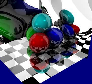
71 3.5 Radiosity Radiosity techniques compute the energy transfer based on diffuse radiation between different surface components (e.g. polygons, triangles, ) of a scene. By incorporating diffuse reflections from all different objects within the scene, we get a quite different effect in terms of ambient lighting. This can be particularly important, for example for interior designers. The correlation between different objects are described by integral equations, which are approximated to find the solution. The total emitted energy (radiosity) is then used as input for the rendering method. In order to integrate specular reflection, radiosity can be combined with raytracing. 3-71

72 3.5 Radiosity Radiosity incorporates the propagation of light while observing the energetic equilibrium in a closed system. For each surface, the emitted and reflected amount of light is considered at all other surfaces. For computing the amount of incoming light at a surface we need: The complete geometric information of the configuration of all emitting, reflecting, and transparent objects. The characteristics with respect to their light emitting properties of all objects. 3-72

73 3.5 Radiosity Let S be a three-dimensional scene consisting of different surface elements S = { S i }. and E the emitted power per surface E(x) [ W/m 2 ] in every point x of S. The surfaces with E(x) 0 are light sources. We then are interested in the radiosity function B(x) [W/m 2 ] which defines the (diffuse) reflected energy per surface. This can then be used to determine color values and render the scene. 3-73

74 3.5 Radiosity Energy transport x θ x θ y B ( x) = E( x) + ρ( x) F( x, y) B( y) dy ρ( x) [0,1] S Reflectivity of the surface S at x cosθ x cosθ y F( x, y) = V ( x, y) 2 π x y Attenuation y Angle of incidence and reflection Visibility (0 or 1) Normalization 3-74

75 3.5 Radiosity If the equation describing the energy transport is discretized, for example using the B-spline basis functions to express the functions E(x) and B(x) E( x) = e = ibi ( x) B( x) i we can derive from the integral equation B ( x) = E( x) + ρ( x) F( x, y) B( y) dy a system of linear equations b i = e i + ρ i j f ij b j S i b B ( x) i i 3-75

76 3.5 Radiosity The coefficients e i of the emitting function E(x) and the reflectivity coefficients ρ i of the individual surfaces segments S i are known. The ρ i describe the material properties, which determine which part of the orthogonally incoming light is reflected. The form factors f ij determine the portion of the energy that is transported from S j to S i and depend only on the geometry of the scene. The form factors can be computed using numerical integration across the hemisphere observing the size, direction, and mutual visibility of the surface segments S j and S i. 3-76

77 3.5 Radiosity Computation of the form factors using numerical integration for a differential surface da i : Hemisphere, Nusselt 81 Hemicube, Cohen

78 3.5 Radiosity Computation of the form factors The form factors between the differential surfaces da i and da j of the surface segments S j and S i result in: i dfij = vij 2 v ij : visibility cosθ cosθ π r (1 if da j visible from da i, 0 otherwise) The form factors of S j to S i equal to cosθ = i cosθ j fij vij 2 π r S S i j j da j da j da i 3-78

79 Radiosity The resulting system of linear equations can then be described as: Or in matrix form: This system is usually solved separately for the different frequencies of light (e.g. RGB). = j i j ij i i e b f b ρ = n n nn n n n n n n n e e e b b b f f f f f f f f f M M L M O M M L L ρ ρ ρ ρ ρ ρ ρ ρ ρ

80 3.5 Radiosity Rendering a scene Computation of the radiosity values b i for all surface segments S i Projection of the scene and determination of the visibility Computation of the color values for each pixel Comments: For different views, only the steps two and three need to be repeated Step three can be accelerated by interpolating along scanlines For step one, the form factors f ij need to be calculated before the system of linear equations can be solved. 3-80

81 3.5 Radiosity Sub-division of a scene The finer the sub-division of the scene into surface segments the better the results. However, the number of form factors increase quadratically and the size of the system of linear equations increases linearly with an increasing number of surface segments. In addition, approximation of the integral equation using the system of linear equations only works for constant radiosity per surface segment. Sub-division is required for critical (non-constant) areas. 3-81

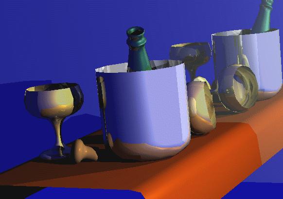
82 3.6 Texture mapping Motivation So far, all surfaces (polygonal objects or free-form surfaces) were modeled as idealized, smooth objects in contrast to real-world surfaces with lots of detail. The explicit modeling of surface details is too costly for rendering and is therefore simulated using different mapping techniques. In the beginning, plain texture mapping [Catmull 1974] was introduced, which projected two-dimensional structures and patterns (textures, consisting of texture elements, texels) onto the surfaces of the objects. Several variations were then developed on top of this technique. 3-82

83 3.6 Texture mapping Principle 3-83

84 3.6 Texture mapping Comments: We usually distinguish between two different approaches: forward and inverse mapping In practice, it proved useful to split up the mapping process into two steps (for example for the forward mapping): 1. First, the texture is projected onto an interim object using a simple mapping s-mapping Rectangles, cubes, cylinders, or spheres are often used 2. Then, the texture is mapped onto the object that is to be texturized o-mapping 3-84

85 3.6 Texture mapping Example: interim objects 3-85

86 3.6 Texture mapping Example: interim objects Planar Sphere Cylinder 3-86

87 3.6 Texture mapping Approaches to o-mapping 1. Reflective ray 2. Objekt center 3. Normal vektor 4. Normal of interim object 3-87

88 3.6 Texture mapping Inverse mapping using interim objects Object space Image plane Interim object Texture plane 3-88

89 3.6 Texture mapping When using free-form surfaces (Bézier splines, B- splines), we can use the parameterization of the surface instead of mapping to an interim object. The parameter of a point on the surface is then also a texture coordinate. For triangulated surfaces, we usually define a texture coordinate for every vertex in addition to the normal vector (color information is not necessary in this case since it is overwritten by the texture). During rasterization of the triangles, a texture coordinate is computed for every pixel using linear interpolation (OpenGL does this automatically). Modern graphics hardware often store textures in graphics memory for faster access. 3-89

90 3.6 Texture mapping Aliasing Texture mapping is very sensitive to aliasing artifacts: A pixel in image space can cover an area of several texels. On the other hand, a texel of the texture can cover more than one pixel in the resulting image. Textures are often patched together periodically, in order to cover a larger area. If the sampling rate is to low aliasing artifacts occur. Oversampling, filtering, interpolation (instead of sampling), level-of-detail 3-90

91 3.6 Texture mapping Bump mapping Texture mapping simulates a textured but planar/smooth surface. In order to simulate a rougher surface and make it appear more three-dimensional, bump mapping does not change the surface geometry itself but changes the normal vectors that are used by the lighting model: Simulation of surface bumps on top of planar surfaces by changing the normal vectors. 3-91

92 3.6 Texture mapping Bump mapping Bright Dark Incoming light reflected light a smooth planar surface appears evenly bright an arched surface appears darker when facing away from the viewer 3-92

93 3.6 Texture mapping Bump mapping The change ΔN of the normal vector N is done in a procedural fashion or by using a texture map. This change can, for example, be described by a gray-level texture. The gradient of this texture (interpreted as a scalar field) then gives us the amount and direction of the change ΔN. This way, regular structures (e.g. a golf ball) as well as irregular structures (e.g. bark) can be simulated. When looking at an object that uses bump mapping, it is, however, often noticeable that the surface itself is planar. 3-93

94 3.6 Texture mapping Bump mapping Examples: 3-94

95 3.6 Texture mapping Displacement mapping On top of the surface, a height-field is used, which moves the points of the surface in direction of the normal vector. This technique also changes the shape of the surface making it no longer planar. 3-95

96 3.6 Texture mapping Opacity mapping / transparency mapping Using opacity mapping, the alpha-value of a transparent surface can be changed locally. The object, for which opacity mapping is used, can be changed according to the used texture in its entirety or only locally. 3-96

97 3.6 Texture mapping Procedural mapping An algorithmic description, which simulates bumps or unevenness, is used to change the surface of an object. This is often used, for example, for 3-D textures. 3-97

98 3.6 Texture mapping 3-D (texture) mapping Instead of a 2-D image, a 3-D texture (volumetric image) is used and usually mapped onto a series of planes. wood grain marble 3-98

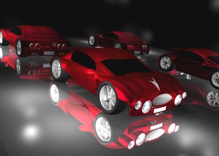
99 3.6 Texture mapping Environment mapping Environment mapping simulates realistic mirroring effects of the (virtual or physical) environment surrounding the object. This way, a complex surrounding can be integrated as a photo-realistic image, without explicitly modeling the surrounding. An interim objects (sphere, cube) is used to project the environment on. Nowadays, this is supported by current graphics hardware. environment texture viewer 3-99

100 3.6 Texture mapping Environment mapping Examples: 3-100

101 3.6 Texture mapping Environment mapping Examples: 3-101

102 3.6 Texture mapping Chrome / reflection mapping An arbitrary two-dimensional pattern is mapped onto a reflecting surface. The texture itself stays fixed at a certain location in 3-D space. Often blurriness is used to achieve more realistic effects

103 3.6 Texture mapping Example: chrome / reflection mapping + ray-tracing 3-103

104 3.6 Texture mapping Comments: Different types of mapping techniques can be combined and applied to the same surface. This is supported in most commercial rendering and animation tools. Most of these techniques can be implemented on the graphics hardware (after appropriate pre-processing) achieving rendering in real-time. See, for example, NVIDIA s FX Composer:

105 3.7 OpenGL illumination and surface rendering Light sources OpenGL supports up toe eight light source (GL_LIGHT0 through GL_LIGHT7). To enable lighting you need to issue: glenable (GL_LIGHTING) Each light source can be enabled using, for example: glenable (GL_LIGHT0) Properties of light sources can be changed using the command: gllight* (lightname, lightproperty, propertyvalue); 3-105

106 3.7 OpenGL illumination and surface rendering Properties Different properties are available: Location: Color: GLfloat position [] = { 0.0, 0.0, 0.0 }; gllightfv (GL_LIGHT0, GL_POSITION, position); GLfloat color [] = { 1.0, 1.0, 1.0 }; gllightfv (GL_LIGHT0, GL_AMBIENT, color); gllightfv (GL_LIGHT0, GL_DIFFUSE, color); gllightfv (GL_LIGHT0, GL_SPECULAR, color); 3-106

107 3.7 OpenGL illumination and surface rendering Attenuation: gllightf (GL_LIGHT0, GL_CONSTANT_ATTENUATION, 1.5); gllightf (GL_LIGHT0, GL_LINEAR_ATTENUATION, 0.75); gllightf (GL_LIGHT0, GL_QUADRATIC_ATTENUATION, 0.4); Spot lights: GLfloat direction [] = { 1.0, 0.0, 0.0 }; gllightfv (GL_LIGHT0, GL_SPOT_DIRECTION, direction); gllightf (GL_LIGHT0, GL_SPOT_CUTOFF, 30.0); gllightf (GL_LIGHT0, GL_SPOT_EXPONENT, 2.5); 3-107

108 3.7 OpenGL illumination and surface rendering Material properties Different kind of materials can be generated with regard to, for example, their shininess using glmaterial*: GLfloat diffuse [] = { 0.2, 0.4, 0.9, 1.0 }; GLfloat specular [] = { 1.0, 1.0, 1.0, 1.0 }; glmaterialfv (GL_FRONT_AND_BACK, GL_AMBIENT_AND_DIFFUSE, diffuse); glmaterialfv (GL_FRONT_AND_BACK, GL_SPECULAR, specular); glmaterialf (GL_FRONT_AND_BACK, GL_SHININESS, 25.0); 3-108

109 3.7 OpenGL illumination and surface rendering Normal vectors Normal vectors can be provided by using the command glnormal*: GLfloat normal [] = { 1.0, 1.0, 1.0 }; GLfloat vertex [] = { 2.0, 1.0, 3.0 }; glnormal3fv (normal); glvertex3fv (vertex); Make sure that the normal vector is provided before the vertex since OpenGL is a state machine! If your normal vectors are not normalized OpenGL can do that for you if you issue: glenable (GL_NORMALIZE); 3-109

110 3.8 OpenGL texture functions Creating the texture and copy it to the graphics memory: GLuint image []; unsigned int width = 256, height = 256; glteximage2d (GL_TEXTURE_2D, 0, GL_RGBA, width, height, 0, GL_RGBA, GL_UNSIGNED_BYTE, image); Enable textures: glenable (GL_TEXTURE_2D); If you use OpenGL prior to version 2.0 width and height have to be powers of two! 3-110

111 3.8 OpenGL texture functions Texture coordinates Provide a texture coordinate for every vertex of you polygonal mesh: GLfloat texcoord = { 1.0, 1.0 }; GLfloat vertex = { 2.0, 1.0, 3.0 }; gltexcoord2fv (texcoord); glvertex3fv (vertex); Again, provide the texture coordinate before the vertex! When using vertex arrays, texture coordinates can also be provided as a single array: GLfloat texcoordarray; glenableclientstate (GL_TEXTURE_COORD_ARRAY); gltexcoordpointer (ncoords, GLfloat, 0, texcoordarray); 3-111

112 3.8 OpenGL texture functions Naming textures If you use more than one texture you need to provide names in order to be able to switch between the provided textures. GLuint texname; glgentextures (1, &texname); Then, you can change between them using these names: glbindtextures (GL_TEXTURE_2D, texname); Remember, OpenGL is a state machine so it will use this texture from now on for every texture related commands! 3-112