Image and Multidimensional Signal Processing

Size: px

Start display at page:

Download "Image and Multidimensional Signal Processing"

Abel Conley
5 years ago
Views:

1 Image and Multidimensional Signal Processing Professor William Hoff Dept of Electrical Engineering &Computer Science

2 Representation and Description 2

3 Representation and Description After segmenting an image to find regions of interest, we want to represent those regions in a concise form This can be used for Recognition Compression Further processing (e.g., joining, simplifying, tracking) Two main approaches Boundary based methods Region based methods 3

4 Boundary Representations We want a compact representation of the boundary of a binary region, to support recognition Methods: Chain codes Fourier descriptors 4

5 Boundary-based Representations Chain codes Follow the boundary around a region Record the direction of travel Yields a sequence of numbers that can be stored concisely, or used for recognition Problems Chain codes can be long Small disturbances in the boundary can cause large changes in the code Solution We can resample on a larger grid spacing 4-directional 8-directional 5

6 start Examples Resulting code: Resulting code: We can redefine the starting point so that the resulting sequence of numbers forms an integer of minimum magnitude 6

7 Relative Direction Can normalize for rotation by looking at the relative turning direction at each point Also the same as taking the first difference of the chain code 0: Go straight 1: turn left 3: turn right 7

Fourier Descriptors Represent the boundary by a sequence of points (assume clockwise order) { (x 0,y 0 ), (x 1,y 1 ),, (x K-1,y K-1 ) } Write each point [x(k),y(k)] as a complex number s(k) = x(k) +

8 Fourier Descriptors Represent the boundary by a sequence of points (assume clockwise order) { (x 0,y 0 ), (x 1,y 1 ),, (x K-1,y K-1 ) } Write each point [x(k),y(k)] as a complex number s(k) = x(k) + j y(k) Take 1D Fourier transform of s(k) to get coefficients a(u) K 1 a( u) s( k) e k0 j2 uk / K Fourier descriptors are a concise description of (object) contours Can be used for Contour processing (filtering, interpolation, morphing) Image analysis (characterizing and recognizing shapes) 8

9 Fourier Descriptors We have Fourier transform coefficients a(u) K 1 a( u) s( k) e k0 j2 uk / K Given coefficients, we can reconstruct boundary K 1 1 s( k) a( u) e K u0 j2 uk / K What is a(0)? Higher order coefficients can be truncated for a more concise representation (e.g., low pass filter) Other filters: Sharpening, edge extraction,... 9

10 Matlab Example First find boundary points (use bwtraceboundary) Take FFT, and truncate higher order coefficients Take inverse FFT, and plot resulting contour (Images from 10

11 clear all close all % Read in a silhouette image I = imread('tool088.gif'); imshow(i,[]); pause % Find a starting point on the boundary [rows cols] = find(i~=0); contour = bwtraceboundary(i, [rows(1), cols(1)], 'N'); % Subsample the boundary points so we have exactly 128, and put them into a % complex number format (x + jy) samplefactor = length(contour)/128; dist = 1; for i=1:128 c(i) = contour(round(dist),2) + j*contour(round(dist),1); dist = dist + samplefactor; end C = fft(c); % Chop out some of the smaller coefficients (less than umax) umax = 32; Capprox = C; for u=1:128 if u > umax && u < 128-umax Capprox(u) = 0; end end % Take inverse fft capprox = ifft(capprox); % Show original boundary and approximated boundary figure, imshow(imcomplement(bwperim(i))); Colorado hold on, School plot(capprox,'r'); of Mines 11

object can be recognized irrespectively of its position, size and orientation Example

12 Fourier descriptors for recognition Need to make Fourier descriptors invariant to common transformations (translation, changes in scale, rotation) Then the contour of a known object can be recognized irrespectively of its position, size and orientation Example application classify leaves From: Berlin University of Technology lecture on Fourier descriptors 12

Transformations Consider these transformations of the contour in the image plane Rotation, translation, scaling Shifting the starting point of the sequence These result in simple transformations of

13 Transformations Consider these transformations of the contour in the image plane Rotation, translation, scaling Shifting the starting point of the sequence These result in simple transformations of the Fourier transform Rotating the contour is equivalent to multiplying the Fourier transform by e jq Translating the contour just affects the 0 th coefficient Scaling the contour is equivalent to multiplying the Fourier transform by the same factor Changing the starting point of the sequence to point k is equivalent to multiplying the Fourier transform by e -j2ku/n 13

14 Transformations Can normalize a Fourier descriptor vector for rotation, translation, scaling, and starting point Set a(0) = 0 => puts centroid at the origin Set all a(u)=a(u)/ a(1) => normalize for scale Normalization with respect to rotation and starting point is a little more complicated, but can be done A simple way is to just discard the phase information and just take the magnitudes of the Fourier descriptors (i.e., the spectrum) This isn t the best way, though, because different shapes can have the same Fourier spectrum (Information loss, both shapes have the same amplitude spectrum) 14

15 Example Rotate and scale one of the images, compare the Fourier descriptors clear all close all I1 = imread('tool005.gif'); imshow(i1,[]); % Find a starting point on the boundary [rows cols] = find(i1~=0); Step 1: extract Fourier descriptors of first image, normalize for translation and scale contour = bwtraceboundary(i1, [rows(1), cols(1)], 'N'); % Subsample the boundary points so we have exactly 64, and put them into a % complex number format (x + jy) samplefactor = length(contour)/64; dist = 1; for i=1:64 c1(i) = contour(round(dist),2) + j*contour(round(dist),1); dist = dist + samplefactor; end C1 = fft(c1); C1(1) = 0; % Put centroid at the origin C1 = C1 / abs(c1(2)); % Normalize for scale 15

16 Example % Make rotated, scaled, and translated version scale = 1 + (0.5-rand); I2 = imresize(i1,scale); ang = 90*(0.5-rand); I2 = imrotate(i2, ang); figure, imshow(i2,[]); Step 2: extract Fourier descriptors of second image, normalize for translation and scale % Find a starting point on the boundary [rows cols] = find(i2~=0); contour = bwtraceboundary(i2, [rows(1), cols(1)], 'N'); % Subsample the boundary points so we have exactly 64, and put them into a % complex number format (x + jy) samplefactor = length(contour)/64; dist = 1; for i=1:64 c2(i) = contour(round(dist),2) + j*contour(round(dist),1); dist = dist + samplefactor; end C2 = fft(c2); C2(1) = 0; % Put centroid at the origin C2 = C2 / abs(c2(2)); % Normalize for scale 16

17 Example figure, plot(1:64, abs(c1), 1:64, abs(c2)); Step 3: compare the Fourier descriptors for the two images... since only the phases are different, the magnitudes should be the same Now try comparing the Fourier descriptors for two different images 17

18 Regional Representations Describe a segmented region using concise features Can use representation for recognition We have already looked at describing boundaries using Chain codes Fourier descriptors Now we look at describing the interior Statistical moments Texture measures 18

19 Statistical Moments The (p th,q th ) image moment is Note: p q mpq, x y f ( x, y) m 00 = area Centroid is: m x m m y m ( x, y) R ( ( x) f ( x, y) y) f ( x, y) f ( x, y) f ( x, y) R 19

20 Moments Central moments (subtract means) p, q x y p x y y x f ( x, y) q Normalized central moments (divide by area raised to a power) p, q where p, q 0,0 p q 2 1, for p q 2,3, 20

21 Principal Axes Major and minor axes are the eigenvectors of M Eigenvalues l 1,l 2 are the lengths ê 1 l l2 E e e e e ê 2 ME E Matlab s regionprops computes these 21

22 I = imread('tool088.gif'); [L,n] = bwlabel(i); stats = regionprops(l, 'all'); bb = stats(1).boundingbox; imshow(i, []); rectangle('position', bb, 'EdgeColor', 'g'); pause; See Matlab s regionprops cx = stats(1).centroid(1); cy = stats(1).centroid(2); major = stats(1).majoraxislength/2; minor = stats(1).minoraxislength/2; ang = -stats(1).orientation*pi/180; imshow(i, []); line([cx-major*cos(ang) cx+major*cos(ang)],... [cy-major*sin(ang) cy+major*sin(ang)], 'Color', 'g'); line([cx-minor*cos(ang+pi/2) cx+minor*cos(ang+pi/2)],... [cy-minor*sin(ang+pi/2) cy+minor*sin(ang+pi/2)], 'Color', 'y'); pause; cp = stats(1).convexhull; imshow(i, []); hold on; plot(cp(:,1), cp(:,2), 'g'); 22

23 Hu s Invariant Moments Combinations of moments are invariant to translation, scale, and rotation Can be used for recognition f 1 = η 20 + η 02 f 2 = (η 20 η 02 ) 2 + (2η 11 ) 2 f 3 = (η 30 3η 12 ) 2 + (3η 21 η 03 ) 2 f 4 = (η 30 + η 12 ) 2 + (η 21 + η 03 ) 2 f 5 = (η 30 3η 12 )(η 30 + η 12 )[(η 30 + η 12 ) 2 3(η 21 + η 03 ) 2 ] + (3η 21 η 03 )(η 21 + η 03 )[3(η 30 + η 12 ) 2 (η 21 + η 03 ) 2 ] f 6 = (η 20 η 02 )[(η 30 + η 12 ) 2 (η 21 + η 03 ) 2 ] + 4η 11 (η 30 + η 12 )(η 21 + η 03 ) f 7 = (3η 21 η 03 )(η 30 + η 12 )[(η 30 + η 12 ) 2 3(η 21 + η 03 ) 2 ] (η 30 3η 12 )(η 21 + η 03 )[3(η 30 + η 12 ) 2 (η 21 + η 03 ) 2 ]. 23

24 24

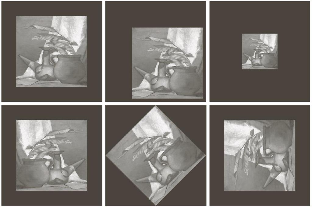
25 Texture Segment an image based on texture Example application: Autonomous road following 25

26 Texture Analysis Examples of texture Representations: Statistical, structural, spectral Images from the Brodatz photo album, commonly used for evaluating texture recognition algorithms 26

27 Statistical Descriptions of Texture Mean, variance, and higher order moments Derived values: R-value (is zero for uniform areas, 1 for areas with large variation) 1 R Uniformity U L 1 i 0 p 2 ( z i ) Entropy e L 1 i0 p( zi )log 2 p( z i ) 27

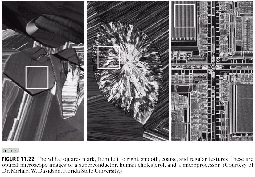
28 28

29 Example Statistical measures of smooth, coarse, and regular textures Notes: Third moment indicates skew of histogram to the left or right of the mean 29

30 Co-occurrence Matrices We consider not only the distribution of intensities, but also their relative positions Compute a 2D histogram of pixel pairs (a co-occurrence matrix), where H(a,b) = # occurrences of gray level a being at a certain relative location to gray level b a r,q b In general, H(a,b; r,q) 30

31 Example Let relationship = neighbor immediately to the right g ij = # times intensity j is to the right of i i j j i 31

32 Example Compute a co-occurrence matrix for the following image with gray levels 0,1,2 Consider a relative position of one pixel to the right and one pixel down image Co-occurrence matrix G 32

33 A highly correlated image will yield high values along the diagonal Co-occurrence matrices ( one pixel to the right ) 33

34 Interesting Results from Human Vision Experiments on what types of texture humans can discriminate pre-attentively (without cognitive processes) Julesz conjecture: Textures that have the same first and second order statistics are indistiguishable Statistics: First order statistics: measures of single points (mean, variance, density) Second order statistics: measure of pairs of points at different relative positions (co-occurrence values, co-variance) 34

35 Difference: size & firstorder statistics Difference: orientation & second-order statistics 35

36 identical second-order but different third- and higher-order statistics 36

37 Counter Examples Some textures with identical 1 st and 2 nd order statistics can be discriminated These involve conspicuous local features, called textons Our visual system can pre-attentively group these This is an example of structural texture representation 37

38 Texton features Color Terminator, number of end-of-lines. Ex. Closure, Connectivity Elongated blobs of different sizes. Ex. Granularity 38

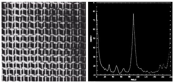
39 Spectral Approaches Sum energy in bins corresponding to ranges of spatial frequencies This can detect regular patterns or patterns at certain orientations 39

the main energy not associated with the background is along the

40 Example The periodic bursts of energy in both spectra are due to the periodic texture of the coarse background In this spectra, the main energy not associated with the background is along the horizontal axis, corresponding to the strong vertical edges in (b) 40

41 S( r) S( q ) q 0 R 0 r1 S q S r ( r) ( q ) 41

42 f(x,y) F(u,v) S(r) S(q) 42

43 S(q) 43

44 Summary / Questions Two methods to represent the boundary of a region are (1) chain codes, and (2) Fourier descriptors. Two methods to represent the region itself are (1) statistical moments, and (2) texture measures. What types of texture measures are there? 44

Lecture 8 Object Descriptors

Lecture 8 Object Descriptors Azadeh Fakhrzadeh Centre for Image Analysis Swedish University of Agricultural Sciences Uppsala University 2 Reading instructions Chapter 11.1 11.4 in G-W Azadeh Fakhrzadeh