Centre for Operational Research and analysis

Transcription

1 Centre for Operational Research and analysis

2

3 A User Guide to Tyche Version 3.0 Converting Tyche to a Modern Development Environment Cheryl Eisler Centre for Operational Research and Analysis Defence Research and Development Canada CORA Technical Memorandum DRDC CORA TM April 2013

4 Her Majesty the Queen in Right of Canada, as represented by the Minister of National Defence, 2013 Sa Majesté la Reine (en droit du Canada), telle que représentée par le ministre de la Défense nationale, 2013

5 Abstract.. Tyche is a Monte Carlo discrete-event simulation software tool developed by Defence Research and Development Canada s Centre for Operational Research and Analysis (DRDC CORA) to support the Royal Canadian Navy in conducting capability-based planning for force structure analysis. To broaden the application of Tyche to a joint environment and improve the performance of the software, DRDC CORA has established a requirement to transition the Tyche software to a fully-supported, modern programming language. In the first stage of the upgrade to Tyche 3.0, the programming language was converted from Microsoft Visual Basic 6.0 to Microsoft Visual Studio 2010 (Visual C#.NET ). This document contains the updated user guide for Tyche 3.0. It is designed to help program users to become familiar with the Tyche tool and set up, run, and review a simulation step-by-step. Throughout this user guide, a simple force structure example is used as a tutorial to illustrate how Tyche 3.0 works. Résumé... Tyche est un outil logiciel de simulation à événements discrets de type Monte Carlo développé par le Centre d analyse et de recherche opérationnelle de Recherche et développement pour la défense Canada (CARO RDDC) pour appuyer la Marine royale canadienne dans ses tâches de planification fondée sur les capacités aux fins de l analyse de la structure de la force. Afin d élargir l application de Tyche à un environnement interarmées et améliorer la performance du logiciel, le CARO RDDC a déterminé qu il était nécessaire de faire passer le logiciel à un langage de programmation moderne jouissant de tout le soutien voulu. À la première étape de la mise à niveau à Tyche 3.0, le langage de programmation est passé de Microsoft Visual Basic 6.0 à Microsoft Visual Studio 2010 (Visual C#.NET ). Le présent document contient le guide de l utilisateur mis à jour pour Tyche 3.0. Il est conçu pour aider les utilisateurs du programme à se familiariser avec l outil Tyche et configurer, lancer et revoir une simulation étape par étape. Dans tout le guide de l utilisateur, un exemple simple de structure de la force est utilisé en tant que tutoriel pour illustrer comment Tyche 3.0 fonctionne. DRDC CORA TM i

6 This page intentionally left blank. ii DRDC CORA TM

7 Executive summary A User Guide to Tyche Version 3.0: Converting Tyche to a Modern Development Environment Cheryl Eisler; DRDC CORA TM ; Defence Research and Development Canada CORA; April Introduction: Tyche is a Monte Carlo discrete-event simulation software tool that was developed by Defence Research and Development Canada s Centre for Operational Research and Analysis (DRDC CORA) to support the Royal Canadian Navy in conducting capability-based planning for force structure analysis. In the interest of broadening the application of Tyche to a joint environment (i.e., across all services of the Canadian Armed Forces) and the need to increase both simulation speed and capability, DRDC CORA established the requirement to transition the Tyche software to a fully-supported, modern programming language [1]. The first stage of the upgrade was a direct language conversion from Microsoft Visual Basic 6.0 to Microsoft Visual Studio 2010 (Visual C#.NET ) based on the recommendation from [2]. Results: The Tyche tool now has three software components: the Tyche Graphical User Interface (GUI), the Simulation Manager (SM), and the Simulation Engine (SE). CAE Integrated Enterprise Solutions completed the programming for the back-end functionality of the GUI and SM, provided routine maintenance, and assisted with the update of the contents of the help files. This document contains the updated user guide for Tyche 3.0. It is designed to help program users to become familiar with the Tyche tool and set up, run, and review a simulation step-by-step. Throughout this user guide, a simple force structure example using notional data will be used as a tutorial to illustrate how Tyche 3.0 works. Significance: The conversion of Tyche to a more modern language like Visual C#.NET means that the tool is implemented in a fully-supported, integrated development environment that will enable use for several years to come. Also, the reliance on outdated and problematic ActiveX controls in earlier versions of Tyche has been eliminated. Preliminary testing of the SE [3] has indicated that the average simulation run times on comparable data sets have been halved, thus increasing the performance of the software. This will enable modelling of larger and more complex problems, as well as better explore solution search spaces to determine more optimal solutions. Future Plans: Now that the original functionality of the tool has been reproduced, advanced functionality can be added, such as modification of the hard-coded timescales to user-selectable timescales, inclusion of Theatre-to-Theatre distances, refinement of the asset selection algorithm, implementation of a user-selectable assignment heuristics, and redesign of the event handler so that it allows for modeling of concurrent operations, waypoints/forward basing, and alternative locations for events. It is also recommended that the help files and user guides be constantly maintained as the software evolves. DRDC CORA TM iii

8 Sommaire Un guide de l'utilisateur pour Tyche version 3.0 : convertir Tyche à un environnement de développement moderne Cheryl Eisler; CARO RDDC TM ; Recherche et développement pour la défense Canada CARO; avril Introduction : Tyche est un outil logiciel de simulation à événements discrets de type Monte Carlo développé par le Centre d analyse et de recherche opérationnelle de Recherche et développement pour la défense Canada (CARO RDDC) pour appuyer la Marine royale canadienne dans ses tâches de planification fondée sur les capacités aux fins de l analyse de la structure de la force. En vue d élargir l application de Tyche à un environnement interarmées (c.-à-d. dans tous les éléments des Forces armées canadiennes) et pour accroître la vitesse et la capacité des simulations, le CARO RDDC a déterminé qu il était nécessaire de faire passer le logiciel Tyche à un langage de programmation moderne et jouissant de tout le soutien voulu [1]. La première étape était une conversion directe du langage de Microsoft Visual Basic 6.0 à Microsoft Visual Studio 2010 (Visual C#.NET ) en fonction de la recommandation de [2]. Résultats : L outil Tyche a maintenant trois composants logiciels : l interface graphique, le gestionnaire de simulation et le moteur de simulation. CAE Integrated Enterprise Solutions a fait la programmation pour les fonctions d arrière-plan de l interface graphique et du gestionnaire de simulation, a procédé à de la maintenance de routine et a prêté son assistance pour la mise à jour du contenu des fichiers d aide. Le présent document contient le guide de l utilisateur mis à jour pour Tyche 3.0. Il est conçu pour aider les utilisateurs du programme à se familiariser avec l outil Tyche et leur permettre de configurer, lancer et revoir une simulation étape par étape. Dans tout le guide de l utilisateur, un exemple simple de structure de la force est utilisé en tant que tutoriel pour illustrer comment Tyche 3.0 fonctionne. Signification : La conversion de Tyche à un langage plus moderne tel que C#.NET signifie que l outil est mis en oeuvre dans un environnement de développement intégré avec tout le soutien voulu, ce qui permettra son utilisation pendant de nombreuses années à venir. De plus, la dépendance à des contrôles ActiveX désuets et problématiques est éliminée. Des tests préliminaires du moteur de simulation [3] indique que le temps d exécution d une simulation moyenne avec des ensembles de données comparables a été réduit de moitié, ce qui améliore donc la performance du logiciel. Cela permet de modéliser des problèmes plus grands et plus complexes, et de mieux explorer les espaces de recherche de solutions afin de déterminer les solutions optimales. iv DRDC CORA TM

9 Plans d avenir : Maintenant que la fonctionnalité originale de l outil a été reproduite, des fonctions avancées peuvent être ajoutées, par exemple le remplacement des échelles de temps figées dans le code par des échelles de temps que l utilisateur peut choisir, l inclusion de distances de théâtre à théâtre, le perfectionnement de l algorithme de sélection des ressources, la mise en œuvre d une heuristique d affectation configurable par l utilisateur et une reconception du traiteur des événements qui permet une modélisation d opérations simultanées, l établissement de points de cheminement et de bases avancées et le recours à des emplacements de rechange pour des événements. Il est aussi recommandé que les fichiers d aide et les guides d utilisateur soient tenus à jour au fil de l évolution du logiciel. DRDC CORA TM v

10 Table of contents Abstract..... i Résumé i Executive summary... iii Sommaire... iv Table of contents...vi List of figures... x List of tables... xiii Acknowledgements... xiv 1 Introduction Background Developmental History Requirements for new development Aim Scope Outline Advantages, applications, and limitations of Tyche Modelling capabilities of Tyche Modelling limitations of Tyche Installing and starting Tyche Version System requirements Installation guide Start-up User s guide to the Tyche GUI Parent window Data Entry Environment Capabilities Bases Theatres Asset Types Asset Name Asset Category Asset Levels Multi-Level Constraints Asset Type Bump Table Force Structures Scenarios Scenario Name Scenario Location vi DRDC CORA TM

11 Scenario Phases Capability Demand and Search Domain Scoring Criteria View Ideal Assets Scenario Types Saving data to a file Run environment Run in debug mode Force Structure Iterations Number of Years Random Seed List of Scenario Types Apply Specialized Lift Capability Rules Generate Statistics Run buttons Running a Monte Carlo discrete event simulation (MCDES) Simulation initialization Creation of a discrete list of events Assigning and registering Assets to events Run output to a.tyo file Operational Schedule environment OpSched Viewer panel organization and axis titles Asset OpSched pane Mission OpSched pane Alternate colour schemes Alternate background color Viewing Iterations Search Function Search mode Search buttons Search results display Save search results to file Data Analysis environment Asset statistics Scenario statistics Capability statistics Risk analysis User s guide to the Simulation Manager The Tyche Simulation Editor Input File DRDC CORA TM vii

12 5.1.2 Ouput Directory Force Structure Iterations Years Random Seed Scenario Types Apply Specialized Lift Capability Rules Simulation control buttons Starting the simulation The Tyche Dashboard Add a new simulation Dashboard settings Maximum Concurrent Simulations Notifications Failure Timeout Administering all simulations Dashboard window management Administering individual simulations Force Pause Resume Abort Clear Open Output View Log Duplicate Edit Input File Debug Applet tray icon and toolbar Conclusions and future work References Annex A Definition of the Asset Types used in the tutorial A.1 JSS A.2 Multi-Purpose Ship A.3 AAW Module A.4 Battle Group Annex B Entity relationship diagram Annex C Risk analysis workbook C.1 Overview of workbook C.2 Consequence weights C.3 Risk viii DRDC CORA TM

13 C.4 Cumulative risk C.5 Risk breakdown C.6 Risk to CFDS missions C.7 Category C.8 Chart of all vignettes C.9 Chart of major contributors C.10 Macros Annex D Tutorial output files D.1 Asset statistics (.tya) D.2 Scenario statistics (.tys) D.3 Capability statistics (.tyc) Annex E XML log entries List of symbols/abbreviations/acronyms/initialisms DRDC CORA TM ix

14 List of figures Figure 1: Tyche 3.0 executable structure Figure 2: Installation setup wizard Figure 3: Tyche GUI parent window Figure 4: Tyche Help file Figure 5: Blank Data Entry Environment Figure 6: Data Entry Environment with tutorial example data Figure 7: Capability window, showing character error-detection Figure 8: Data Entry Environment with Capabilities Figure 9: Add a new Base Figure 10: Enter the distance from Base to Base Figure 11: Data Entry Environment with Bases entered Figure 12: Add a new Theatre Figure 13: Enter the distance from Theatre to Base Figure 14: Theatre with distances entered Figure 15: Data Entry Environment with a Theatre Figure 16: Edit Asset Type window Figure 17: Selecting values for an Asset Type Figure 18: Edit the Default Level Figure 19: Edit a Level Figure 20: External Asset availability in the Edit Asset Type window Figure 21: External Asset availability in the Edit Level window Figure 22: Condition for a following Level to occur Figure 23: Deployed Level of the JSS, partially completed form Figure 24: Multi-Level Constraints window Figure 25: Add Force Structure Figure 26: Data Entry Environment with one Force Structure Figure 27: Add New Scenario window Figure 28: Add Phase window Figure 29: Event scheduling for a Phase with one follow-on Phase Figure 30: View Ideal Assets function x DRDC CORA TM

15 Figure 31: Right-click on View Ideal Assets window Figure 32: Data Entry Environment with tutorial Scenario entered Figure 33: Add New Scenario Type window Figure 34: Data Entry Environment with Scenario Types Figure 35: Window used to start a run in debug mode in Tyche Figure 36: Illustration of the list of steps followed for any given iteration Figure 37: Selected time window for events Figure 38: Flow chart describing the logic used by Tyche Figure 39: Matching problem on a bipartite weighted graph Figure 40: Illustration of the backtracking (left) and backjumping (right) processes Figure 41: Illustration of the OpSched Viewer Figure 42: Asset OpSched Viewer information displayed on right-click Figure 43: Mission OpSched Viewer information displayed on right-click Figure 44: Asset Level colouration window Figure 45: Scenario Type colouration window Figure 46: OpSched Viewer with white Asset background Figure 47: Second iteration of tutorial data displayed in the OpSched Viewer Figure 48: Operational Schedule Viewer search function Figure 49: Operational Schedule Viewer search function after a search has been run Figure 50: Sample search text results Figure 51: Options to automatically run statistical analyses Figure 52: Data Analysis Environment window Figure 53: Asset Statistics for the tutorial example for Fleet1, showing average Days Per Year of usage in each Level for each Asset Figure 54: Tyche Simulation Editor Figure 55: Select an output directory Figure 56: Tyche About window Figure 57: System Info window Figure 58: The Tyche Dashboard (Simulation and Queue Monitor) Figure 59: Dashboard Settings window, with defaults shown Figure 60: Simulation context menu on right-click Figure 61: A queued simulation Figure 62: The Debugger window DRDC CORA TM xi

16 Figure 63: The Dashboard applet tray icon with menu and balloon message Figure A-1: Parameters used to define the JSS Asset Type Figure A-2: Maintenance Level for the JSS Asset Type Figure A-3: Deployed Level for the JSS Asset Type Figure A-4: Parameters used to define the Multi-Purpose Ship Asset Type Figure A-5: Maintenance Level for the Multi-Purpose Ship Asset Type Figure A-6: Deployed Level for the Multi-Purpose Ship Asset Type Figure A-7: Parameters used to define the AAW Module Asset Type Figure A-8: Deployed Level of the AAW Module Asset Type Figure A-9: Parameters used to define the Battle Group Asset Type Figure A-10: Deployed Level of the Battle Group Asset Type Figure B-1: Entity relationship diagram for Tyche Figure C-1: Consequence weights spreadsheet Figure C-2: Screenshot of empty risk table Figure C-3: Screenshots of risk (a) and failure probability (b) graphs for individual Scenario Phases Figure C-4: Screenshot of the risk graph for individual impact categories Figure C-5: Screenshot of the remainder of the Cumulative Risk spreadsheet Figure C-6: Screenshot of the risk breakdown by categories of Capability failure Figure C-7: Screenshot of Risk to CFDS Missions spreadsheet Figure C-8: Screenshot of the cumulative risk by numbered CFDS missions for the CFDS fleet Figure C-9: Screenshot of the Category spreadsheet Figure C-10: Screenshot of chart of all vignettes contributing to risk for CFDS fleet Figure C-11: Chart of major contributors to risk for the CFDS fleet xii DRDC CORA TM

17 List of tables Table 1: Tyche GUI menu commands Table 2: Brief description of Tyche Scoring Criteria Table 3: Sample partial simulation output file, formatted in columns for easier viewing Table 4: OpSched search functionality Table 5: OpSched searches in tutorial example Table 6: Information provided by scenario statistics Table 7: Information provided by Capability statistics Table 8: Available simulation commands Table C-1: Risk analysis workbook tabs Table C-2: Risk, variance and error for each of the impact categories Table E-1: Log entry index DRDC CORA TM xiii

18 Acknowledgements The author would like to recognise the contributions of previous user guide authors: Dr. Dave Allen, Alain Forget, Dave Heppenstall, and Pawel Michalowski [4]-[6]. Laura Avery from CAE Integrated Enterprise Solutions updated the help files for the new version of the software [7] under the Task Authorization entitled CORA Task 147: Tyche 3.0 Graphical User Interface and Simulation Manager Functionality for contract #W /001/SV to Defence Research and Development Canada s Centre for Operational Research and Analysis. xiv DRDC CORA TM

19 1 Introduction 1.1 Background Introduced to the Department of National Defence (DND) in the late 1990s, Capability-Based Planning (CBP) was formally adopted by the Canadian Armed Forces (CAF) as a methodology for force development in Tyche is a Monte Carlo discrete-event simulation software tool that was originally developed by Defence Research and Development Canada s Centre for Operational Research and Analysis (DRDC CORA) in To support the Royal Canadian Navy (RCN) in conducting CBP for force structure analysis and to continuously improve the decision-making process for force development, DRDC CORA s Maritime Operational Research Team (MORT) has invested in the long-term development of the Tyche simulation model. The model has also been examined for use in the larger strategic context for the CAF as a whole [8] and is currently being evaluated by the Strategic Planning Operational Research Team for supporting the assessment phase of the CBP process. Tyche is a stochastic simulation model that schedules assets within a proposed force structure to missions as they occur within a defined threat environment. The threat environment is characterized by a realistic set of missions, each with a specific capability demand and occurring at an estimated frequency, to which the RCN must respond. By understanding the impact of the force structure s capabilities and composition on the RCN s ability to meet the anticipated mission demand, the RCN is better able to make force structure and capability mix investment decisions. Tyche helps to provide such insight by simulating a large number of time periods in which realistically random, concurrent and geographically distributed missions are scheduled [4], representing a variety of outcomes. Assets are assigned to each mission following a set of predefined rules to reproduce the decision making process of a force structure scheduler. The entire process is capability-based, meaning that each mission has a set of capability requirements, and each asset in the force structure has an assessed set of capabilities it supplies. Assets are assigned to missions so that an assigned combination will best meet the capability requirements of the mission. The average performance of a candidate force structure over time indicates the likelihood of the force structure to be able to provide sufficient capability to meet the scheduling requirements under a degree of uncertainty. By repeating the process with different force structure compositions, the performance of each candidate force structure can then be compared. Essentially, capability-based models specify the amount of capability that would be required by the force structure to meet the future capability demanded by missions. Each capability requirement is matched, if possible, to capability resident within assets of a given force structure and the capability match or deficit thereof, is noted and various performance metrics can be computed. In contrast, platform-based force structure models that were used in the past (such as FleetSim [9] or the Air Force Structure Analysis (ASTRA) model [10]), specify specific asset requirements for missions and typically only provide insights with regard to the required number of a given type of unit. Capability-based models like Tyche are thus better designed to perform capability-gap analysis, support platform-capability design, prioritize future capability requirements, and supply quantitative comparisons that can be used for decision support recommendations as to near term capital and operations and maintenance resource allocations. DRDC CORA TM

20 1.2 Developmental History Initially, Tyche was developed by MORT as a tool to compare the performance of various naval force structure options. Tyche Version 1.0 [11] was used for the first naval Fleet Mix Study (FMS I) [12] to identify the minimum number of assets in each proposed ship class that met a maximum acceptable political risk threshold, where political risk was defined as a new measure of performance for the force structure. Because of the length and difficulty of running simulations at the time, only 100 fleets were examined. Tyche was significantly overhauled to produce Version 2.0 [4], which expanded the scope of the model beyond naval ships to a joint, modular, capability-based environment. Subsequent, incremental upgrades provided the ability to queue and manage a large number of simulations on multiple core processors [5], significantly reducing simulation management and run time. Tyche Version 2.2 was primarily used to conduct FMS II in [13]. Over 1,000 fleet options were examined; however, due to the lengthy Monte Carlo process, only a subset of many possible solutions could be found using a heuristic (direct) search method for the optimal fleet. Tyche Version 2.3 saw the simulation engine split out from the Tyche graphical user interface [6], as well as the introduction of comprehensive error handling and context-sensitive help files. Tyche Version 2.3.4, with minor bug fixes and code changes, was the latest stable update released. 1.3 Requirements for new development There are several areas of improvement that were identified for Tyche The primary driver is that all past versions of Tyche up to and including Version have been implemented in Microsoft Visual Basic 6. Due to the fact that Microsoft no longer supports this version of Visual Basic, and a number of issues arising with outdated ActiveX components, a fullysupported, more modern programming language was deemed necessary for future versions. The second area of improvement was the need to increase both simulation speed and capability. Long simulation run times led to restricted search spaces in optimization studies and limited modelling fidelity. By switching to a faster processing language with more efficient data structures, the simulation speed could be reduced. Additional performance increases could also be realized by taking advantage of parallel processing in a high-performance computing environment. In the interest of broadening the application of Tyche to a truly joint environment (i.e., across all CAF services) where the problem space is much larger, simulation run times must be reduced; therefore, Tyche was split into several parts for significant restructuring [3] and upgrade [14]. The Tyche tool previously had four software components: the Simulation Engine (SE), the Graphical User Interface (GUI), the Tyche Dashboard, and the Extensible Mark-up Language (XML) Editor.Microsoft Visual Studio (Visual C#.NET ) was identified as the most suitable development environment and programming language for the Tyche SE [2]. To maintain the highest level of compatibility, Visual C#.NET was also selected for the revision of the remainder of the software. The Dashboard and XML Editor were also to be combined into one executable: the Simulation Manager (SM). Figure 1 illustrates the calling structure of the executables required for Tyche 3.0, simplifying the execution and management of the code within Visual C#.NET. The GUI was to remain the user interface for input file development and 2 DRDC CORA TM

21 analysis of simulation output. From the GUI, the user should be able to either call the SE as a standalone executable or run the same code (for debugging purposes) through the GUI. When the SE is called as a standalone executable, the SM should also be called to manage all instances of the SE that may be running at the same time; additional simulations can then be started from the SM, creating new instances of the SE. The ability to call the SE directly from the command line prompt must exist for integration with high performance computing systems, which will again trigger the SM to watch over the queue. The SM should also have the ability to locate the input file associate with a simulation output, and open the file using the GUI. Tyche SM Tyche GUI Tyche SE Debugging Code Tyche SE Tyche SE Tyche SE Tyche SE Tyche SE Tyche Can be called from command line Figure 1: Tyche 3.0 executable structure. 1.4 Aim This user guide explains how and why to use Tyche 3.0. The advantages of the modelling and analysis tool are presented in relation to existing DRDC CORA tools; as well, specific limitations on use are articulated. Once the reader understands the applicability of the model at hand, the program itself is introduced. The document is designed to help program users to become familiar with the Tyche tool and set up, run, and review a simulation step-by-step. A simple force structure example will be used as a tutorial to illustrate how Tyche 3.0 works. The Tyche Version 2.0 User Guide [4] was used as the basis for the updated user guide. The document structure is updated to reflect the changes from Tyche Version 2.0 to Version 3.0. Content was also incorporated from [15], [5], [6], and [16]. 1.5 Scope This document is a user guide for Tyche 3.0 and also describes the structure, logic, inputs, and outputs of the program, without detailing programming elements that are non-essential to the generic user. The programmer s guide is available electronically as part of [7]. DRDC CORA TM

22 1.6 Outline Section 2 presents a detailed discussion of the advantages and limitations of Tyche for specific modelling and analysis applications. Section 3 indicates how to install the program for use on a desktop personal computer. The Tyche GUI is introduced in Section 4 for the program user to enter the data required to perform simulations. The SM, covered in Section 5, can be used to perform batch processing of unattended simulations. The SE performs the simulations and outputs the resulting data and statistics files; it is called by the GUI and SM as required. For more information on the SE, the reader is referred to the Programmer s Guide (parts 5 through 7) in the Tyche 3.0 help files [7]. A short summary of recommendations for future work are presented in Section 6. Annexes cover additional detail of the tutorial example input and output, of the automated risk analysis that was added to Tyche, and of log entry options. 4 DRDC CORA TM

23 2 Advantages, applications, and limitations of Tyche 2.1 Modelling capabilities of Tyche Tyche is a Monte Carlo discrete-event simulation tool built around a capability-based scheduling model for quantitative force structure evaluation. Force structure evaluation models are typically focused on the performance assessment of a particular combination of assets, often modelling to a moderate or high degree of fidelity (i.e., how closely the model represents the rules used in the processes that are modelled) the asset specifications, required military missions to be carried out by those assets, and the conditions under which the assets should operate. The primary outputs are a detailed assessment of the risk associated with scenarios that cannot be completed by the force structure and the capability deficiencies of the forces structure. [17] This means that at its core, Tyche utilizes capabilities as its fundamental unit of trade; matching asset supply to scenario (mission) demand, based on availability and scheduling heuristics. This scheduling model is constructed as a discrete-event simulation, maintaining a list of events that are processed for every iteration of the simulation such that a) no foreknowledge of the future is available, and b) only those time steps in the simulation with events are processed. The simulation utilizes multiple iterations in a Monte Carlo fashion, so as to obtain random values from specified distributions for input variables for each iteration. Each iteration is different, and the average risk assessment across all iterations provides an indicator of the force structure s performance. Because of how the model is designed, Tyche is capable of [8]: Modelling assets with varying levels of capability usage and their own capability demand (for example a Frigate sent with a Helicopter has a higher Anti-Submarine Warfare capability than without [13]); Modelling external assets (representing those available from a non-dnd source, such as a charter company), which can be generated with a probability of availability specified by the user; Applying timing and occurrence constraints across or within levels of usage of assets to represent personnel tempo constraints, for example; Defining bases and theatres in terms of relative distances, not real-world locations. This abstracts the problem to minimize the data required, can reduce the classification of the dataset, and allows for generalization to land, air, sea and space assets; Generating scenarios stochastically to better mimic real-world conditions (there is no restriction on the number or type of concurrent missions); Defining scenarios with multiple theatres, each with a specified probability of occurrence; Splitting scenarios into phases; where phases can be defined as random, scheduled or follow-on events, the latter with a specified probability of occurrence or based on a minimum duration of the preceding phase (capturing conditional events, such as quality of life breaks when operations are longer than six months in duration); DRDC CORA TM

24 Accommodate a variety of scheduling constraints by overlapping or offsetting scenario phases in their timing; Prioritizing scenarios so as to assign assets to more important scenarios first, when more than one occurs at the same time; Assigning assets to scenarios based on factors in the capability matched between supply and demand, with a possible penalty applied for excess above the matched capability. Two additional Scoring Criteria can be applied to tailor how the assets are chosen for the scenarios: timeliness into theatre and scheduling conflict. When sufficient scenario timing information is entered and the specific scenario deadlines are introduced, timeliness penalties and thresholds can be factored in. In terms of scheduling conflict, penalties and thresholds can be applied once scenario priorities are established; Applying instructions directed at completion of rescheduled events regarding unfinished time; Assigning assets within a force structure to events dynamically and chronologically, utilizing the policy to meet a single requirement by selecting from a list of available assets based on information that is known and actionable at the moment a mission occurs [18]; Allowing for various levels of fidelity (such as availability constraints, maintenance requirements, rotation ratios, readiness levels, personnel tempo constraints, quality of life breaks, failures, etc.), depending on the depth of the study required; Applying and tailoring heuristics that mimic the decisions a real force structure scheduler would make; Utilizing quantitative metrics for relative comparison of force structures (capability-based and risk-based measures [19]); Producing data that can be analyzed using add-ons to compute the concurrency of scenario occurrences [20] and the concurrency of asset usage [21]; Being run inside an optimization framework [13] to help determine the best structure to satisfy the capability requirements. This would allow for the decision makers to set multiple, possible conflicting, objectives and an algorithm could be used to find to optimal solution to meet those objectives; and Being run from the command line prompt as a console application for the SE, permitting batch processing through the Tyche SM and submission of jobs through a high-performance computing system. The software tool has undergone continuous improvement for well over a decade by DRDC CORA [2],[3]-[6],[11],[23] -[27], with a significant portion of the effort spent on verification and validation. While there are other DRDC CORA tools that can be utilized in a capability-based fashion for force structure analysis, they are either too generalized or too specialized to provide the right level of detail for long-term, strategic level force structure planning which is Tyche s niche. For example, the Stochastic Fleet Estimation (SaFE) / SaFE Robust (SaFER) / SaFE under Steady State Tasking (SaFESST) trio of tools make such simplifying assumptions that the force structure size will always be underestimated [17]; albeit good for when fast answers are needed for 6 DRDC CORA TM

25 minimum estimates. On the opposite end of the spectrum, The Managed Readiness Simulator (MARS) tool [28] is designed more for operational level planning, as it requires fixed parameters for upcoming missions (no demand uncertainty) and operates down to individual personnel. 2.2 Modelling limitations of Tyche There are several important points to remember when considering any study that employs Tyche [8]: Combat attrition is not accounted for; The capability of an asset is constant over time. Degradation and/or damage cannot be directly modelled; The composition of a force structure is constant over time. New assets cannot be introduced and existing assets cannot be removed or retired; Repeating events within Tyche are generated based on the frequency and distribution type assigned to them. Any rescheduling of a single event does not affect future events in the series, thus schedule slippage does not occur; and Assets must deploy from predefined bases (one home base for each asset). Waypoints and forward deployments cannot be modelled. The first three limitations can be mitigated by modelling assets with reduced capability sets or force structures with assets removed. The average steady-state performance can then be compared to show how incremental losses would impact the system. Dramatic decreases over short periods of time could not be assessed. In terms of waypoints and forward deployments, unless the details of the routing are critical to the problem, in many cases these can safely be ignored or accommodated in a generic scheduling case. For example, if an asset must travel to a waypoint, wait, and resume travel, this can easily be modelled by reducing the overall speed of the asset, so that it arrives in theatre at the time it would be expected after the original travel routing. A case that could not be accommodated would be if the Asset must undergo some maintenance (represented by an asset level) at the waypoint that must be tracked and reported on. DRDC CORA TM

26 This page intentionally left blank. 8 DRDC CORA TM

27 3 Installing and starting Tyche Version System requirements Before installing and running Tyche 3.0, it is important to ensure that the following system requirements are met. Tyche 3.0, like its predecessors, is a Microsoft Windows -based program which is designed to run on personal computers, as well as in a Windows -based highperformance computing environment. Tyche 3.0 can run on systems with the Windows 7 or later operating system (earlier/alternative systems were not tested and did not form part of the operational requirement). The minimum suggested system requirements include a 1.5 Gigahertz (GHz) processor 1 with 386 Megabytes (MB) of Random Access Memory (RAM) to be able to install and run Tyche. When the user intends to run simulations locally with output data being saved to the hard drive, it is recommended to have at least 2 Gigabytes (GB) of free disk space. Before the user can install Tyche, they must ensure that the Microsoft.NET Framework 4.5 (as a minimum) is already installed on their system. Without the Framework, the software will not run. The user is also recommended to have Microsoft Excel and WinZip 9.0 or later, with the Command Line Support Add-On. While these latter two programs are not strictly required, they are useful for batch processing of simulation runs (as will be discussed in Section 4.5). 3.2 Installation guide Tyche 3.0 comes as a zipped file ( Tyche.zip ) that can be unpacked to any location on a user s computer. When the file is unzipped, the setup executable ( setup.exe ) should be run to install Tyche. The setup wizard shown in Figure 2 will guide the user through the process. When the setup wizard asks for a location to install the program, the user must select a folder where they have full control. If the default location (under C:\Program Files or C:\Program Files (x86)) is read-only for the user, a different location MUST be selected or special permission must be granted. 1 The simulation run time scales down linearly with Central Processing Unit (CPU) speed, so a faster computer will have faster simulation run times. Therefore, it is recommended to use as high a CPU speed as possible. In addition, the use of hyper threading and turbo boost (on Intel processors) is also highly recommended. AMD processors are not recommended, as Tyche simulations run significantly slower on them than Intel processors for comparably rated CPU speed. DRDC CORA TM

28 Figure 2: Installation setup wizard. Once installation is complete, the user will be asked to restart the computer. System file registration and file type association will be completed upon restart. 3.3 Start-up After the setup wizard has completed the installation process, there are three executables that are installed: the Tyche GUI, SE and SM. The main point of entry for the user is the Tyche GUI, which can be run on a personal computer in several ways. From the Windows Start Menu, under All Programs, there will be a folder called Tyche 3.0. The user can click on the Tyche shortcut here to open the GUI, or navigate through Windows Explorer to the installation directory and double-click on the executable file ( Tyche.exe ). The Tyche SM is designed to run in the background all of the time, and automatically runs on computer start-up in the system tray once installed. The novice user is recommended to become familiar with the GUI and develop an input file before progressing to the Tyche SM. The Tyche SE is designed to run silently as a console application and will either be called by the GUI, the SM, or directly by a more advanced user familiar with the command line prompt calls required. The SE will not be discussed in detail in this document; for more information on the SE, refer to the Programmer s Guide sections in the Tyche 3.0 help files [7]. 10 DRDC CORA TM

29 4 User s guide to the Tyche GUI 4.1 Parent window The Tyche GUI is used for the modification of input files and the viewing of output files; it is called by the user as necessary. The first display which appears upon running the Tyche GUI is the empty parent window illustrated in Figure 3. Figure 3: Tyche GUI parent window. The toolbar functions and menu commands at the top of the parent window provide access to the GUI application s main functionalities. The toolbar is separated into two sections, one for file handling and another for functional environments. For complete menu descriptions, refer to Table 1. Menu items are presented in the order in which they would normally be used. The four environments listed under the View menu and shown at the top right of the toolbar in Figure 3 indicate the primary uses for the Tyche GUI. The Data Entry Environment is used to input all data and save input files. The Run Environment enables setup of parameters to control and perform a simulation run. The OpSched Viewer Environment allows for graphical viewing of the output from a simulation run. The Data Analysis Environment is used to perform various statistical analyses on a simulation run. Within the Tyche GUI, the environments are presented in the order in which they would ordinarily be used. Each of the environments will be discussed in detail in the subsequent sections. DRDC CORA TM

30 MENU/SUBMENU File Table 1: Tyche GUI menu commands. DESCRIPTION The File menu contains file input/output access commands. Common shortcuts to these commands are replicated on the file handling section of the toolbar. View Data Entry The Data Entry Environment displays all information from an input file. When the user opens a file, this environment window is displayed in the parent window automatically. Tools Help Run OpSched Data Analysis Confirm All Cancellations Run in Debug Mode When pressed, either the Run Environment window or the Tyche SM opens (based on the preference selected under Tools see below under Tools > Run in Debug Mode) in order to start a new simulation for an input file. The Operational Schedule Viewer Environment allows users to graphically view the asset assignment choices made during a completed simulation run. The Data Analysis Environment allows the user to perform a statistical analysis on an output file generated from a simulation. When checked, the user will be asked to confirm if changes have been made to the input file when the cancel button is pressed. When unchecked, this option will allow the user to cancel without being asked to confirm if changes have been made. When checked and the Run Environment is selected, the Run window will open, allowing the user to run a simulation directly from the GUI. This is typically used for debugging purposes. When unchecked and the Run Environment is selected, a simulation will be started through the Tyche SM. The Help menu contains context-sensitive help (a sample of which is shown in shown in Figure 4), 2 a reference to application documentation, and version information. 2 A compiled hypertext mark-up (CHM) help file provides context-sensitive help with the [F1] key. Help files were originally written in hypertext mark-up language (HTML) and compiled into a single.chm file using Adobe RoboHelp. The.chm files are included with the executables, and can be accessed through the Tyche Help menu using Contents, Index or Search to bring up a separate help window. When the user presses the [F1] key while a window is active, the topic linked to that window will then be displayed. 12 DRDC CORA TM

31 4.2 Data Entry Environment Figure 4: Tyche Help file. The input of data into the Tyche GUI is done through the Data Entry Environment, which may be accessed by creating a new input file or opening an existing input file. Tyche input files carry a.tyi file extension. This can be accomplished using the File menu, or by clicking on the New File button or Open File button in the toolbar at the top of the Tyche parent window (Figure 3). Figure 5 shows the Data Entry Environment window with a newly created input data file. Figure 5: Blank Data Entry Environment. The Data Entry Environment features toolbars positioned along the top of the window and a resizable interface, which will increase or decrease the size of individual columns within the window respectively. Here, the user is able to enter or modify data in each of the following columns: Capabilities, Asset Types, Force Structures, Bases, Theatres, Scenarios and Scenario DRDC CORA TM

32 Types (to be described in sub-sections to 4.2.7, respectively). The currently-selected column list in the Data Entry Environment is highlighted in yellow, and when a list is populated, the individual column menu buttons for New, Edit, Copy, and Delete functions will become enabled. At this point, a tutorial example using notional data will be developed to step the user through the data entry process, as well as provide a concrete example of inputs for a simulation. The example will illustrate some of the unique modelling features within Tyche and be accompanied by recommendations for the user when developing their own simulations. The tutorial example is comprised of land (a Battle Group), sea (Joint Support Ship (JSS) and Multi-Purpose Ship classes), and modularized (a containerized Anti-Air Warfare (AAW) Module) Assets to illustrate a simple joint force structure problem. The data defining these four Asset Types and all their associated Levels are given in Annex A. The following sub-sections will discuss how to enter the data. These Asset Types are hypothetical and the capabilities attributed to these Assets do not model the capabilities of real CAF assets. To illustrate Tyche s flexibility, a Battle Group and an AAW Module are included in the example. The AAW Module is a Plug & Play concept module that can be installed aboard a Multi-Purpose Ship to provide an increased Air Defence Capability to this ship that it otherwise would not have. With this Capability, the Multi-Purpose Ship will be able to protect a nearby JSS against air threats. A single Force Structure will be modelled, comprised of one or more of each Asset Type, with two possible Bases (Halifax and Esquimalt) for each Asset to be stationed at. One Scenario is defined (Sc9) to attend at a specified Theatre (Location1), of a Peace Keeping type. The Scenario Demand is linked to Asset supply via seven capabilities: Interdiction, Self-Defence, Plug-In, Air Defence, Lift, Sustainment, and Peace Keeping. There is a strong dependence between the various Asset Types: the Multi-Purpose Ship requires Sustainment, a Capability that is provided by the JSS which requires Air Defence, a Capability provided by the AAW Module which requires Plug- In Capability, a Capability provided by the Multi-Purpose Ship. Figure 6 illustrates the Data Entry Window with the tutorial example data entered. 14 DRDC CORA TM

33 Figure 6: Data Entry Environment with tutorial example data Capabilities Since Tyche is capability-based, it is suggested to begin data entry for any new input file with the Capabilities. Capabilities simply refer to any ability to perform a task; the level of detail and exact representation for the Capabilities within a given simulation are left to the discretion of the user. For example, a strategic level Capability might be Command and Control, whereas a tactical level Capability might be Ability to Carry a Semi-Automatic Rifle. The Capability might be abstracted away from the Assets which provide them, in a one-to-many relationship (where one Asset may bring multiple Capabilities to Theatre), or they might maintain a one-to-one ratio (where one Capability corresponds to one Asset). The selection of Capabilities is what links the Capability Supply from the Assets to the Capability Demand from the Scenarios how the user chooses to define the Capabilities depends upon the minimum number of relationships that are necessary to be modelled to establish the right assignment in the schedule. This may not seem entirely straightforward to a new user; however, this is where careful planning and a bit of creativity is required ahead of time to plan out what the user is trying to model. To add a new Capability, click on the Add New Capability button found at the top left of the window, under the Capabilities heading. The user can enter text for the name of the Capability in the dialog box that appears; it also features built in error-detection. If the user inputs invalid data (such as a vertical slash, semi-colon ; or comma, ; see Figure 7), the user will not be permitted to click the OK button. He or she will be presented with a flashing exclamation point and an error message until the error is corrected. This same error checking is applied to all textual fields within Tyche, as these three special symbols are utilized within the input and output files for formatting data. DRDC CORA TM

34 Figure 7: Capability window, showing character error-detection. The data from the tutorial example will now be utilized to illustrate data entry and manipulation. In the Capability Name field, type in the name of a new Capability. For this example, first enter Interdiction. When satisfied with the name of the Capability, click on the OK button to save the new Capability. To complete the example list of Capabilities, in the same manner as before, enter the following additional Capabilities: Self-Defence, Plug-In, Air Defence, Lift, Sustainment, and Peace Keeping. Figure 8 displays the Data Entry Environment window after all the aforementioned Capabilities have been entered. Figure 8: Data Entry Environment with Capabilities. Note that each of these Capabilities has very different physical implementations. For example, Self-Defence could be provided by a torpedo launcher on a ship, while Peace Keeping might be provided by an army unit comprised of personnel and all related equipment and armament required to enforce peace between hostile nations. If one is not concerned with modelling the individual components of a system (such as the individual torpedo launchers), the Capability can neatly summarize a complex set of relationships or requirements in a black box (i.e., Self Defence provided by a ship) as long as the right boxes (ships) are sent to the Scenario, then the scheduling requirements will be satisfied. 16 DRDC CORA TM

35 If the name of a Capability needs to be modified, the user may edit the Capability by clicking on the Capability Name and then clicking on the Edit button below the Capabilities heading or by pressing the Enter key. Alternatively, simply double-clicking on the Capability Name also allows the user to edit the Capability. Note that the Capabilities whose Names start or end with the term Lift (such as Sealift or Airlift) are treated in a different way than the other Capabilities. An option exists before a simulation is run to allow the user to apply specialized assignment rules to Assets that only provide such Lift Capabilities to a mission. Normally, all Capabilities required for a mission are assumed to be needed for as long as the mission lasts. If selected, only the Lift Capabilities are treated differently, and they are assumed to be required only at the beginning and at the end of the mission (see Subsection for a discussion of the mission Capability Demand). This represents delivery and pickup of items at the start and finish of a mission. To delete a Capability, click on the Capability, and then press the Delete button Capabilities heading or press the Delete key. below the In the Data Entry Environment Capability list, the order of items can be changed by right clicking on the item and dragging it into place. For example, the user could move the Air Defence Capability to the top of the list by right clicking on Air Defence and dragging it to the top of the Capability list. In the case of Capabilities, the list order is not relevant to the simulation; this is more for the preference of the user. However, there will be cases where order is important, and these will be discussed subsequently Bases Next, the locations at which the Assets can be based must be defined. Bases are used to provide departure and return locations for Assets at the start and end of every mission (Scenario occurrence). Bases are comprised of a Name and the Distance between it and any other point location defined in the model. These locations include both Bases and Theatres; a Theatre is a location where a mission (Scenario) can take place. It is very important to note that the units for the Distance have not been specified, nor will they be explicitly. The user must maintain internal data consistency such that the selected unit is compatible with the Speed unit that will be associated with the Asset Types (see Section 4.2.4) assigned to that Base. For example, if the Speed is entered in knots then the Distance should be in nautical miles (nm), or if the Speed is in kilometres per hour then the Distance should be in kilometres. Distances are purely relative within Tyche. There is no map to work from or routing to specify. The user must calculate the necessary distance for the Assets to travel based on whatever considerations are important to the simulation to be run. One apparent issue with this, for example, is that the air distance is usually very different from the sea distance. For instance, a ship will travel about 7500 nm to go from Victoria to Halifax (as it must travel through the Panama Canal) while the straight-line distance by air is about 2500 nm by great circle route. Which of the two distances should be entered? The answer is both, if one is modelling both types of Assets. Tyche 3.0 is capable of handling both at the same time, if the user puts all air assets at different Bases from sea assets. The distance from a Base housing air assets to any Theatre would be an air distance while sea distances would be used for the distance from a sea base to any DRDC CORA TM

36 Theatre. So, even though an air and a sea base may be physically collocated in reality, separation in modelling allows for different relative travel distances. The same would apply to land assets. What is important in the end is the travel time to theatre that is computed as a result, which impacts the scheduling of the assets. To create a new Base, the user presses the Add New button below the Bases heading in the Data Entry Environment. Figure 9 displays the Base window, ready for data input. Note that the OK button is inactive until a Name is entered. Simply entering the name of the Base is sufficient to create the Base at this stage in the example. For now, enter Halifax in the Name field. Since there is currently no Base or Theatre input into the system yet, the lists of To Bases and To Theatres are empty. Otherwise, all of the Bases and Theatres would be listed there, and the user would be required to enter the distance from this new Base to each of the other Bases and Theatres. See section for creating Theatres and inputting distances. Press the OK button. Figure 9: Add a new Base. Using the same procedure as before, create a second Base named Victoria, but now the distance between Bases must also be entered. Before exiting the Add New Base window, click on the Edit Distance to Base button or double-click on Halifax in the list of Bases to launch the Distance From Base to Base window in Figure 10. Enter the distance from Victoria to Halifax as Click the OK button to save the distance, and then click the OK button in the Add New Base window to save the new Base. Figure 11 shows the Data Entry Environment window with the names of the new Bases in the list of Bases. Figure 10: Enter the distance from Base to Base. 18 DRDC CORA TM

37 Figure 11: Data Entry Environment with Bases entered Theatres Next to be created are the Theatres. As mentioned, a Theatre is a point location where a mission (Scenario) can take place. It is important to note here that Tyche is focused on the scheduling of Assets to and from Theatre it does not take into account any activities that occur during a mission, in Theatre. Once an Asset arrives, it is assumed to fulfil its role, it then stays for the duration of the Scenario (or less depending on conflicting events), and then returns to Base. A Name and the travel Distance separating it from the various Bases define a Theatre. For every Base-Theatre pair, there must be a Distance value. After inputting a Theatre Name, the user must specify the distance between this new Theatre and each Base that has already been input. If the Theatres had been created first and the Bases second, all the distances between each new Base and each Theatre would still have to be input. To add a Theatre, press the Add New Theatre button below the Theatres heading in the Data Entry Environment. Figure 12 shows the Theatre window, ready for the input of a new Theatre. Note that it looks similar to the Base window, except that only the To Bases are listed. 3 If no Distance has been specified, the text box will display zero for the Distance. This should only occur when creating a brand new Theatre. Even when creating Theatres that are nominally in the same location as a Base, a minimum value of 1 must be entered, so that the travel time is nonzero. 3 Theatre-to-Theatre Distances are not employed within the Tyche model. DRDC CORA TM

38 Figure 12: Add a new Theatre. For a new Theatre in the tutorial example, input Location1 in the Theatre Name field. Select a Base and then click on the Edit button at the top right of the Specify Distances area or doubleclick on the Base name to edit the distance from Location1 to the Base. Enter the Distance as shown in Figure 13 from Location1 to Halifax, and then press the OK button. Repeat these steps, using 5000 to Victoria. When finished entering the Distance from Location1 to both Bases, Figure 14 results; click the OK button in the Add New Theatre window to store the new Theatre. Figure 15 displays the Data Entry Environment with the list of Theatres now populated with the new Theatre that has been created. When editing a Theatre and changing the Distance from the Theatre to any given Base, the user will find the Base to the Theatre Distance automatically updated afterwards. For example, on the Data Entry Environment window, if Location1 was selected and then Halifax selected in the list of Bases on the Theatre window to be edited, the user should see 3000 in the Distance field of the Distance from Theatre to Base window. If the Distance is changed to 1234, and the user returns to the Data Entry Environment and selects the Base Halifax for editing, 1234 should be the Distance displayed in the To Theatres list of the Edit Base window. Changes made in the Edit Theatre window automatically become reflected in the Edit Base window, and vice versa. Figure 13: Enter the distance from Theatre to Base. 20 DRDC CORA TM

39 Figure 14: Theatre with distances entered. Figure 15: Data Entry Environment with a Theatre Asset Types Because Asset Types are dependent upon both Capabilities and Bases in their definition, they should only be created after the latter two already exist (noting that partial Asset Type development can certainly occur, and models can be worked on in a variety of ways this is simply the easiest route for a beginning user). An Asset Type should be viewed as a representation of a type of object owned or operated by the DND/CAF or an external source that can be called upon to be scheduled to support operations (like a chartered sealift vessel). The Asset Types are distinct from the Assets themselves. For instance, the ship HMCS Toronto is an Asset, whereas the ship class Frigate is an Asset Type. An Asset is an instantiation of an Asset Type and will be introduced in section 4.2.5, where a Force Structure comprised of individual Assets will be built. DRDC CORA TM

40

41 Asset Category There are three Categories of Asset Types that can be selected by using the drop down list appearing in the Asset Type window. The three Categories are: Dynamic, Static and External. The first two are used only for DND/CAF-owned Asset Types. The Dynamic Category should be selected for Asset Types that can get to the Theatre without having to be transported (for example, naval ships). The Static Category should be selected for DND/CAF-owned Asset Types that require transportation to Theatre, such as crews, weapons, smaller vehicles 4 carried by a larger asset, etc. Finally, the External Category is reserved for Asset Types that are not DND/CAF-owned. The operational schedule of external Assets is not thoroughly determined, as it would be for DND/CAF-owned Assets. During a simulation run, for each mission (Scenario instance) independently, Tyche randomly determines how many External Assets are available Based on the probability of availability for the Asset Type. This means that each mission has an equivalent chance of obtaining an External Asset for scheduling; there is not a fixed number of External Assets in the Force Structure. Furthermore, Tyche assumes that the External Assets can get to Theatre independently. 5 Once the user makes a selection of an Asset Type Category, there is a new field that becomes visible if the Asset Type category is either Dynamic or External. This field is the Asset Type Speed, where the default value is 0. For Dynamic and External Assets, this is the typical Speed of the Asset Type used to travel to Theatre noting that all travel to theatre is performed in a single trip; waypoints and stopovers cannot explicitly be accommodated. No specific units are required, but the Speed value (in distance units per hour) must be consistent with the Distances to Theatre for the travel time calculations. A non-negative, non-zero integer Speed must be specified for both Dynamic and External Assets. In Figure 17, JSS has been entered for the name of the new Asset Type and Dynamic has been selected for the Asset Type category. The Speed value assigned is Whose subsequent in-theatre movement is irrelevant to the scheduling problem, under the assumption that they will return to base with the same asset that transported them to theatre initially. 5 Or be transported via some external means that, for all intents and purposes, can be combined into a single External Asset Type model to simplify the problem. DRDC CORA TM

42 Figure 17: Selecting values for an Asset Type Asset Levels An important feature of the Asset Type is the list of Levels. The Levels define all possible states of existence and use for any Asset of a given Asset Type. One way to think about these Levels is to view them as states, and the Assets as finite state machines. An Asset must exist in one of these states or Levels at all times, and there are rules that exist for allowing the change between one state (Level) and another. It is the rules for when and what Level an Asset can go to that form the basis for the scheduling heuristics and the registered list of events 6 in the Tyche simulation. For example, an Asset may go from one Level to another in order to take part in an event, transitioning from an idle Level to an event Level such as training, maintenance or deployment. It is important to note that all travel to and from locations (Bases and Theatres) is included in the Level selected for the event; a separate travel/transit Level does not need to be created. 6 While the creation and handling of events within the simulation will be left for discussion in Section once the user is more familiar with all data elements within the Tyche GUI, it is important to mention here that the registration of certain types of levels will trigger an event to be processed (such as a scheduled maintenance activity). This will be discussed further in Section DRDC CORA TM

43 To provide the user with a more concrete example to work through, a Frigate Asset Type could have the following five Levels: Idle, Maintenance, Training, Trials and At-Sea. These Levels could be interpreted as follows: a. Idle: The Frigate is alongside at homeport ready to be deployed. b. Maintenance: The Frigate is going through a maintenance period and is not available for deployment. c. Training: The Frigate and its crew are performing training exercises and can be deployed after a delay. d. Trials: The Frigate and its crew are at-sea testing various equipment or tactics to ensure their proper functioning or validity. e. At-Sea: The Frigate is currently at-sea performing a specific mission. There is no specified limit to the number of Levels associated with one Asset Type. It is up to the user to specify enough Levels to adequately model the Asset Type in question. These Levels may correspond to military readiness levels, as defined for CAF Assets, or they may form a more complicated structure to elicit the required assignment to a ranked order of priorities of types of possible events. One Level is automatically given a special role: the Default Level. The Default Level specifies the state to which the Asset returns once its participation in an event ends. In the example of the Frigate just given, the Idle Level corresponds to the Default Level such that, when it has no other assignments, the Frigate will return to the homeport, ready to be re-deployed. As seen in Figure 16, an Asset Type is always created with at least one Level the Default Level. The Default Level is different from other Levels in than many of the fields are not editable; this is because the behaviour of the Default Level is fixed it must be a Follow-On Level, with a Bump Rank of 0 and no Constraints of any kind. This is to ensure that the Asset will always return to this Level without restriction; for if there was a restriction, 7 there would not necessarily be any Level for them to go. In Figure 16, next to each Level Name in the list of Levels, there is also a field for Bump Rank. The discussion of Bump Rank will be deferred to Section The user can Add New, Edit,Copy, and Delete a Level using the various buttons offered in the Asset Type window. If the user were to edit the Default Level, a new window would open that looks like Figure 18. This is where the parameters for an individual Level can be entered or modified, which will be discussed in the following sub-sections according to the red circled numbers in Figure 18, respectively. 7 The one qualification on this statement is that Capability Demand can still be required for the Default Level; this input is recommended for advanced users only. It is possible to create a situation where an Asset cannot return to the Default Level if another required asset is not available; in such case the simulation will fail. DRDC CORA TM

44

45 Figure 19: Edit a Level Bump Rank or Availability For Dynamic and Static Asset Types, each Level has a Bump Rank, which determines if the Asset Type can be rescheduled, or bumped, from one Level to another. Bumping is only allowed from one Level to another Level with the same or higher Bump Rank. In this way, an Asset s Levels can be prioritized so that critical tasks will override (or bump) less important tasks. For instance, if an attack against a North Atlantic Treaty Organization (NATO) country occurs, the CAF could remove a Frigate from a training exercise and send it to respond to the attack since participation in NATO collective defence has priority over training activities. In other words, the At-Sea Level (at which the Frigate will be when it goes for NATO collective defence activities) of the Frigate must have a higher bump rank than the Training Level. The Bump Rank is any non-negative integer less than the total number of Levels defined for the Asset Type. This number determines which Levels can bump, and can be bumped by, this Level. The Default Level has a bump rank of 0 to allow the Asset to be bumped from the Default Level to any other Level. DRDC CORA TM

46 For External Asset Types, each Level has an Availability. Because Tyche is not intended to model detailed scheduling of Assets external to the DND/CAF and bumping (rescheduling) does not apply to External Assets, the main concern is whether or not an External Asset is available for use. A list of Levels and probabilistic availabilities is used instead of a list of Levels and Bump Ranks. The Bump Rank is replaced with Availability as shown in Figure 20 and Figure 21, indicating the probability (value between 0 and 1) that a single External Asset is available at any given time for one instance of an event. Figure 20: External Asset availability in the Edit Asset Type window. 28 DRDC CORA TM

47 Figure 21: External Asset availability in the Edit Level window Level Type Under the Name and Bump Rank is the Level Type selection that specifies the conditions under which the Asset Type will be at this Level. There are four possible types: Schedule, Random, On- Demand, and Follow-On. A Scheduled Level Type requires a Start Date (for the first event in the series; in relation to day 0, which is the first day of the calendar year) and Frequency (uniform rate of occurrences per calendar year). A typical scheduled Level is Maintenance. All naval Assets require routine preventive maintenance to ensure their proper functioning. A Random Level Type requires only the Frequency. The occurrence of a Random Level is based on a Poisson distribution with a rate of occurrence (per year) 8 given 8 For further discussion on the generation of events using the Poisson distribution in the simulation, please refer to Section DRDC CORA TM

48 by the entered frequency. This Random Level Type could, for example, be used to simulate ship breakdown events. An On-Demand Level Type is utilized when as Asset is required to attend a Scenario Phase. An example of an On-Demand Level is the Frigate s At-Sea Level. The Frigate would go At-Sea when it is requested to accomplish a given mission. In this case, the user does not have to provide a Start Date or Frequency since the occurrence of the mission is determined by the mission specifics and not by the Asset itself. A Follow-On Level Type is one that can only follow from a previous Level Type; that is, its frequency of occurrence is determined by the occurrence of the previous Level. The Follow-On Level is distinguished from the previous Level by differences in Capability Supply, Demand, Constraints, etc., allowing for modelling and tracking of distinct periods of employment types of a variety of Asset Types. An example of such Level is the Frigate s Trial Level. This Level would follow every Maintenance Level to test the adequacy of the maintenance. Of the four Level Types, Schedule, Random and Follow-On are all utilized to generate Assetdriven events within the simulation. Only the On-Demand Level can be used to respond to Scenario-based events. Depending on the selection, the Start Date and Frequency text boxes (below the Level Type selection) can become enabled Duration The total consecutive amount of time an Asset will spend at a given Level, for each occurrence of that Level in the schedule (i.e. one event), is determined by the Level Type. If it is of a Schedule, Random, or Follow-On (excluding the Default) Level Type, the Duration is generated from a triangular distribution. That is, during a simulation run, for each occurrence of this Level in the event list, a random value is drawn from the triangular distribution with the parameters specified by the user and this value is used as the duration for the event. The minimum, most likely (mode) and maximum values for this distribution are entered in the three text boxes enabled under the label Duration when the appropriate Level Type is selected. In the case where the user has a known duration for an event, the minimum, most likely and maximum values can all bet set to the same value, forcing the distribution to return a single value for the event. On-demand Level Types can utilize only a maximum duration. This maximum duration specifies a constraint on the maximum number of consecutive days the Asset can be at this Level, and applies only to a single event. For example, for an Asset that can be deployed for a maximum of 6 months, the user needs to define an on-demand Deployed Level with a maximum duration of 180 days. If the Scenario requiring the deployment of the Asset lasts for more than 180 days during a single simulation iteration, then the program will search for another Asset to replace the one that was first deployed, to be able to fulfil the rest of the Scenario. 9 9 For more information on asset replacement, refer to Section DRDC CORA TM

49 The Default Level for each Asset Type does not utilize duration information, as there cannot be any constraint on the time spent at this Level Level State The Level State, when enabled, indicates the following Level from the current Level (i.e., what happens when the current event is done) and any conditions for the Follow-On Level to occur. The Default State is to Follow-On with the Default Level, no Constraints. With the exception of the Default Level, all Level Types will have the Following Level enabled and the default set. The list box will only be populated with additional options if other Levels are defined as Follow-On types. If a Level other than the Default Level is selected for Follow-On, the fields Condition for Following Level to Occur and Probability or Minimum Duration will be enabled. The user can choose to leave these fields empty, and the Following Level will always occur. If a particular Condition is selected (either Probability or Minimum Duration), the Probability/Minimum Duration field will then become visible and require a value to be entered, as shown in Figure 22. For Probability, the Following Level only occurs with a probability specified by the user (assuming a uniform distribution); the user must therefore enter a value greater than 0 and less than 1. For Minimum Duration, the Following Level only occurs if the duration of the currentlyedited Level (during an actual simulation iteration) exceeds the minimum duration value specified. Therefore, for Minimum Duration, the user must enter an integer value greater than or equal to 1. Figure 22: Condition for a following Level to occur. Varying the example from the previous sub-section, assume that a Frigate must go through a Trial Level only if the Maintenance is of significant duration (first assuming the Maintenance Level has a duration distribution, for example, of days). This Trial Level will follow a Maintenance Level to test the systems after a specified period of down time. If Minimum Duration is the condition for the Following Level to occur with a value of 12, then the Trial Level will only be scheduled to occur after a Maintenance Level that is at least 12 days long during a simulation iteration. All Maintenance events that are 2 to 11 days in length will be followed by the Default Level Constraints On the top right section of the Level editing window, a list of Constraints can optionally be added to the Level. There are four types of Constraints: 1. Maximum number of days at Level. This essentially limits the total time spent at this Level over a specified interval (in days, evaluated as a rolling window); DRDC CORA TM

50 2. Minimum number of days at Level. This prevents rescheduling of events to ensure that a minimum amount of time is spent at this Level over a specified interval; 3. Maximum number of occurrences of Level. This essentially limits the total number of occurrences of this Level over a specified interval (in days); and 4. Minimum number of occurrences of Level. This prevents rescheduling of events to ensure that a minimum number of occurrences of this Level happens over a specified interval. Such Constraints can be added to any Level, except the Default Level for which no time Constraint can be imposed. Compliance with the Constraints is verified during the run every time an Asset changes Levels. Note: This does not generate new events where none exist. In the minimum case, the data entered must be consistent with the Level Frequency and Duration. In the maximum case, Constraints supersede Level Frequency and Duration parameters. To specify a Constraint, the user first selects the Constrained Parameter. There are two choices of Constrained Parameter: the Occurrence and the Days, with a lower (>=) or upper (<=) bound. Once this has been selected, the user specifies the Limiting Value and the Interval, which must be positive integers. The Interval must also be larger than the Limiting Value. For example, if the user wants to impose that an Asset Type is not deployed more than twice every 12 months (365 days), the following constraint could be entered on the Deployed Level: a. Constrained Parameter: Occurrence b. Upper or Lower Bound: <= c. Limiting Value: 2 d. Over Interval (in days): 365 Once the Constraint has been added, the Constraint appears in a readable fashion in the Constraint List box: Occurrence <= 2/365 (see Figure 23). Considering an Asset Type that cannot deploy more than twice in 12 months, every time an Asset of this type is selected for deployment, Tyche will verify whether or not this particular Asset had been previously deployed twice in the past 12 months. If so, Tyche will look for another Asset of the same type that was not deployed twice in the last 12 months. Alternatively, if the total number of days spent at a Level were to be limited rather than the occurrence, then the user would select Days for the Constraint Parameter. For example, if the limit of days for a Maintenance Level was at least 35 in 365, the user would enter Days >= 35/365 in the Constraint List box. This Constraint stipulates that the Asset must complete at least 35 days of maintenance every year. An Asset with this type of constraint cannot be bumped from a Maintenance Level to perform activities which would ordinarily be considered more important. 32 DRDC CORA TM

51 Figure 23: Deployed Level of the JSS, partially completed form. Care must be taken when adding constraints to a scheduled Level. If, for example, the user limits the occurrence for a Maintenance Level to be 2 times per year or less (occurrence <= 2/365), but the Maintenance Level was scheduled to occur 3 times per year (according to the Frequency), then the last scheduled occurrence of each year will never occur due to the Constraint. In short, the Frequency is superseded by the Constraints imposed on the occurrence of the Level. Note that if the Constraint exceeds the number of Days or Occurrences possible for a given Level, it will simply force the Asset to do all planned Days/Occurrences during the simulation run. It cannot generate new events to make up for the missing Days/Occurrences to meet the Constraint. In the same way, the Duration is superseded by the Constraints imposed on the number of days spent at the Level. For instance, if the user imposes a limit of 50 days of Maintenance per year and 3 maintenance periods are scheduled per year, each one being 20 days long, then the Constraint will reduce the duration of the last maintenance period of each year to 10 days (since the first two are scheduled without constraint violation, and any rolling window for the next year that includes the 10 day maintenance period from the previous will not register a violation, since the total time over the interval will still be 50 days). DRDC CORA TM

52 Capability Supply Capability Supply for the Level is added using the lower left section of the Level Description window. Here, Capabilities can be selected (from the list established in Section 4.2.1) to describe the abilities that the Asset Type possesses (supplies) at the current Level to perform a given task requested from a Scenario or another Asset. The Capabilities are selected from a drop-down list populated with the data entered in Section For each Capability Supply, a Quality and Quantity must be specified. The Quality is a number between 0 and 1 and specifies the extent to which the Capability is provided by the Asset Type. For instance, if there are two different Assets that have some Air Defence Capability, but the sensors and weapons of the first Asset are such that it is able to provide extended range air defence with the same or better success probability than the other Asset, then the first Asset should receive a higher Air Defence Quality value. The exact value is not important as long as the Quality value of the first Asset is higher and a value on the same relative scale is selected for Quality levels in the Capability Demand of the Scenario. In other words, the scale for the Capability Quality when defining between Asset Types is considered a relative ranking rather than an absolute value. The Quantity has to be a positive integer. The Quantity stipulates the integer number of Capabilities that can be simultaneously provided either to a Scenario or another Asset. For example, a ship that can provide Lift might be able to transport 300 similar-sized land forces vehicles simultaneously. In this case, 300 would be the Quantity value associated with the Lift Capability of that ship. If a new land force vehicle were introduced at twice the length of the previous, it could have a Lift Capability Demand of 2, reducing the number of large vehicles that could be carried to 150. Any combination of a mix of sizes could also be transported, as long as the total Quantity value requirement would not exceed Capability Demand The Capability Demand for the Level is added using the lower middle section of the Level Description window. It should list all Capabilities that the Asset Type is required to have to go to the specified Level. For example, a Frigate would require an embarked Crew to go At-Sea. If there is no Crew available to man the ship, then the ship will stay alongside. The manning requirement itself is not given as a Scenario Demand; however the Frigate needs the Crew Asset whenever it is assigned to the At-Sea Level associated with a Scenario. Similar to the Capability Supply, Capability, Quality and Quantity are specified for each Capability Demand. The Capabilities are again selected from a drop-down list populated with the data entered in Section However, now two Quality values (on a scale of 0 to 1) are needed for the Capability Demand. The Required Quality determines the degree of desired Quality for full mission success and the Marginal Quality provides the degree needed for to achieve some acceptable amount of mission success. The Quantity determines the integer number of 10 A similar analogy would be Lego, but in one dimension: say one s supply is the base plate that has 300 of the little pegs/holes on/in it. The demand to build on it would be a variety of blocks. One type of blocks has 6 pegs. How many blocks can your base plate accommodate? DRDC CORA TM

53 Capabilities (in the same units of measure as the Capability Supply) required to support a single Asset of the type being defined. In addition to the Quality and Quantity, the Capability Demand also requires a Weight, which is used to quantify the importance of a Capability Demand with regard to other Capability Demands. 11 Finally, a Capability Demand can also be deemed Essential. If the Essential Capability Demand cannot be satisfied at the Required Quality with a Capability Supply from another Asset, then this Asset will not be able to go to this Level; the Marginal Quality is not used for Essential Capabilities and should be set equal to the Required Quality. For example, for a Frigate to leave a port, it needs to be manned by a Crew. If there is no crew available, then the Frigate will stay alongside. Thus, the Crew provides an essential manning capability that is demanded by the Frigate when it is requested to leave the port. The reverse can also apply: if a Crew is requested to leave the port, but no Frigate is available for the Crew to embark upon, then the Crew is not going anywhere. The Frigate provides an essential embarkation capability that the Crew demands when it is requested to leave the port (air transportation notwithstanding). Tyche has been purposefully designed so that this kind of co-dependent relationship between Assets can be formed. In Tyche 3.0, the user may enter more than one Capability Demand of the same Capability, provided that at least one of the requirements (Quality, Quantity, Weight, or essentiality) is different. This allows the user to model a greater variability of demand, resulting in a more realistic simulation. Taking the Frigate and Crew example further, if the Crew were instead modelled as Sailors, the Frigate may require 180 essential Sailors to man the ship and 50 nonessential Sailors. This would be input as two separate Capability Demands, utilizing the same Capability (manning), provided by the same Asset Type (Sailors). Each sailor would demand one embarkation Capability; the Frigate would provide 220 embarkation Capabilities. Thus the Frigate could sail with anywhere between 180 and 220 Sailors onboard Search Domain for Capabilities In the bottom right corner of the Level editing window is the Search Domain for Capabilities, where the user specifies which Asset Types can fulfill the Capability Demand. The Search Domain is composed of the name of the Asset Type to look for, the Level at which it is requested, and the originating Base. The choice for the Base can be any entered Base or Same as Current Asset. The Search Domain allows the user to accelerate the search process for fulfilling the Capability Demand, rather than having Tyche search through all Asset Types. By exploiting the user s knowledge of the Asset Types, the possible solution set of Assets that can be assigned is narrowed dramatically. If Capability Demands are entered but no Search Domain is specified or the Search Domain contains Asset Types that do not meet the Capability Demands, then Tyche will not find any Assets to meet the Capability Demands. Thus, it is absolutely critical that Asset Types with the proper Capability Supply be entered into the Search Domain. Often, it is better to generate all of one s Asset Types first, and then go back and fill in the Search Domains for 11 Refer to Section for more information on how the Weight is used in the scoring of asset assignments. DRDC CORA TM

54 Capability Demand second. This ensures that all Asset Types are available to populate the dropdown boxes and the user s knowledge of their Capability Supply can be utilized. For example, to man a Halifax-based Frigate requested to go At-Sea, the following Search Domain is appropriate: Asset: Frigate Crew, Level: Deployed, Base: Same as current Asset. That means any Frigate Crew from Halifax that is able to be deployed could man the Frigate. Assets from other Bases would not be considered in this example, as they would have to be transported 12 to Halifax ahead of time. It is here within the Search Domain for Capability Demand that the order of Asset Type with Base choice entry is important. Because the Search Domain defines the space within which Tyche is allowed to search for Capability to supply the demand for the current Asset, it is critical to ensure that the right Assets are a) included in the list and b) entered in the order that reflects the preferences of the user for the purposes of the simulation. Only those Assets included in the list are evaluated (scored) on the capability matching between Supply and Demand, as per Section Once the capability matching is complete and the set(s) of Asset(s) with the highest score has been found, it can be assigned to the event. However, if there is a scoring tie, Tyche will always choose the first Asset in the list of Assets with the highest score. Meaning, if two Assets score equally well, Tyche will chose the one entered first in the list, and then repeat the process of selecting the next best Asset to meet the remaining Demand. Thus, for example, if the user were to assign an implicit evaluation of operating cost to a set of Assets, the Assets should be listed from lowest cost to highest cost to ensure that the least expensive Assets are always chosen first, if the goal were to try to minimize total cost. By defining each Level of an Asset Type with different combinations of characteristics, Capability Supply, and Capability Demand, Asset behaviours and dependencies are defined. In addition, the synergy between Assets in terms of Capability Supply can also be defined. For example, a Destroyer could be defined with two on-demand Levels: Combat Level 1 and Combat Level 2. Say that the Destroyer has some Firing Capability. This Capability can be improved if a Helicopter provides Support to the Destroyer (the Helicopter can, for example, provide an over the horizon link with some surface-to-surface missiles). One can associate a Firing Capability of 0.6 for Combat Level 1 and a Firing Capability of 0.9 for Combat Level 2. However, Combat Level 2 would require a Firing Support Capability provided only by the Helicopter and this Capability Demand would be Essential. Combat Level 2 exhibits the known synergy between the Destroyer and Helicopter, with the increase in Capability Quality provided over the Assets individually. By including both On-Demand Levels in the Search Domain of an Asset or Scenario, Tyche is able to select either the Destroyer/Helicopter combination if they are both available or the Destroyer alone to supply the Firing Capability. It is important to note that Tyche will not discover new Asset synergies or dependencies; it can only exploit those entered as input. 12 Travel time from one base to another for static assets in Tyche is one day, under the assumption that these assets can be flown from base to base in 1 day or less. Travel time for Dynamic/External Asset Types is based on their speed and the Base-to-Base distance. 13 When an Asset is the Source of the Event, the only other Scoring Criterion utilized is Scheduling Conflict; it is a penalty for Assets that are bumped from one Level to another (when Bump Penalties exist). 36 DRDC CORA TM

55 Multi-Level Constraints The Multi-Level Constraints window (Figure 24) allows the user to specify optional Constraints, similar in nature to the Level Constraint (Section ), except that more than one Level can be included in each Multi-Level Constraint. Each Multi-Level Constraint is independent of the others; so one Level may appear in many constraints, as well as retaining its own Level Constraints. Constraints (up to four possible combinations) can be added to impose a maximum or minimum summation of occurrences or days an Asset may be at these Levels. The Multi-Level Constraints are evaluated in the same fashion as Level Constraints, except that the sum of the occurrences or days spent in each included Level for an Asset is used to evaluate whether or not the constraint has been violated before the Asset can be assigned to a Level included in the constraint. To specify a Multi-Level Constraint, the user first selects the Constraints Across Multiple Levels button in the Edit Asset Type window shown in Figure 16. This launches the Multi-Level Constraints window shown in Figure 24. The user will then select the Add New Constraint button under the list of Multi-Level Constraints. The fields on the right side of the window will activate, and the user is required to enter a Name for the Constraint (noting that it cannot be purely numeric characters in the string). Next, just as for the Constraints in Section , the user must select between two choices for a Constrained Parameter: Occurrence or Days. The bound on the constraint can be a lower (>=) or upper (<=) bound. Once these have been selected, the user specifies the Limiting Value and the Interval, which must be positive numbers. The Interval must also be larger than the Limiting Value. Finally, the user must select one or more Levels from the list of available Levels (not including the default Level) for the Asset Type. To save, the user presses the Save button at the top right, inside the Edit Constraint frame. Once the constraint has been added, the constraint name appears in a readable fashion in the Multi-Level Constraints list box. Figure 24: Multi-Level Constraints window. DRDC CORA TM

56 Building upon examples from the previous sub-section, a Destroyer could be defined with two on-demand Levels: Combat Level 1 and Combat Level 2. The user may wish to limit the total number of deployments across both Levels, since restrictions for deployment occurrences are independent of the use of the Helicopter. A Multi-Level Constraint with Occurrence <= 1/545 could be created, with Combat Level 1 and Combat Level 2 as the Levels to include in the Multi- Level Constraint (no individual Level Constraints would need to be created). Every time an Asset of this type is selected for deployment at either Combat Level 1 or Combat Level 2, Tyche will verify whether or not the particular Asset had been previously deployed to either Level in the past 18 months. Every time an Asset of this type is selected for use at any of these Levels, Tyche will verify whether or not the constraint for this particular Asset is respected. If it is not, Tyche will look for another Asset of the same type that does not violate the constraint. Compliance with the Constraints is verified during a simulation run every time an Asset changes Levels. As with Level Constraints, care must be taken when adding scheduled Levels to Multi-Level Constraints. The Duration/Occurrence of a Level is superseded by the Multi-Level Constraints imposed on the Level. Multi-Level Constraints can be deleted by pressing the Delete Constraint button of constraints on the top left, or by pressing the Delete or Backspace key. above the list Asset Type Bump Table Another feature of an Asset Type is the Bump Table, which appears at the bottom of the Asset Type window. In Figure 17, it has one column and one row. However, the table size increases as new Levels are added in the list of Levels; there are as many columns/rows as there are Levels. Each cell of the table provides the data for bumping (rescheduling) the Asset from one specific Level (associated with a column) to another one (associated with the row). This enables the user to model Asset Type-specific rules for scheduling behaviour that a military force structure scheduler might implement. As mentioned above, bumping is allowed only from a given Level to another one when the bump rank of the From Level is equal to or higher than the Bump Rank of the To Level. For this reason, only the cells corresponding to allowed bumps are enabled for data entry. For the enabled cells, a set of three numbers separated by commas is required: 1. The Bump Time specifies the time required for the Asset Type to switch from one Level into another. The Bump Time includes the time required to extract an Asset from its current event and the preparation time required to reach the next Level, not including travel time. Travel time is accounted for separately, based on where the Asset is currently located and where it needs to be. There are four possible cases: If the Asset is currently at a Base and is bumped to a Level that is associated with an event that is occurring in a Theatre, then the Asset must transit from the Base to the Theatre. 38 DRDC CORA TM

57 If the Asset is at a Base and is bumped to a Level that is associated with an event that is occurring at a Base, then the Asset must transit from the current Base to the demanded Base (which may be the same and, as such, the travel time would be zero). If the Asset is in Theatre, and is bumped to a Level that is associated with an event that is occurring in a Theatre, then the Asset must transit from the current theatre, to its home Base and then to the new Theatre. This is one of the few artificialities in Tyche as there is no real world geographic location representation or Theatre to Theatre distance (which could enable the Asset to transit directly from one Theatre to another). Unless one is modelling many long-term, overlapping scenarios with a significant amount of scheduling conflict, the added travel time has negligible effect on the overall schedule. The savings it provides in simplifying the model representation and data entry for the user was considered to be worthwhile trade-off. If the Asset is in Theatre, and is bumped to a Level that is associated with an event that is occurring at a Base, then the Asset must transit from the current Theatre, to its home Base and then to the demanded Base (which may be the same and, as such, the Base to Base travel time would be zero). 2. The Bump Penalty is a value between 0 (no penalty) and 1 (highest penalty) that stipulates the penalty to be given for bumping the Asset Type from its current Level. The Bump Penalty is used when scoring the suitability of a set of Assets for a given mission, and acts specifically as a penalty to Assets that have scheduling conflicts and have to be bumped. The description of the calculation is further explained in Sections and but, essentially, the penalty is intended to influence the asset selection depending on importance of an event assigned by the user. Those events with high importance should be assigned a high penalty, penalizing Assets that are taken from them and rescheduled to another. Events with low importance should be assigned a low penalty, allowing Tyche to freely reschedule Assets between events. 3. The Re-schedule Instruction specifies whether or not the bumped activity needs to be rescheduled. The value of the re-schedule instruction must be 0, 1 or 2. The three Re-Schedule Instruction values denote the following rules: 0: Do not re-schedule the Level. 1: The days of the Level remaining as previously scheduled before the bumping of the Asset, if any, are re-scheduled. This does not affect the scheduling of further events in the series. 2: All missed days of the Level are re-scheduled. This does not affect the scheduling of further events in the series. The difference between the various values is better explained by considering an example. Let us say a Frigate was scheduled to be on Maintenance from day 10 until day 40. Now consider that it is also requested for a mission starting on day 25 and ending on day 35. The Frigate, currently being on Maintenance, needs to be bumped from the Maintenance Level to the At-Sea Level. If the Bump Time is 2 days and the time required for the Frigate to sail from its Base to the Theatre is 1 day, then the ship can get to Theatre on day 28 (=25+2+1) and will come back to home port on day 36 after sailing back for 1 day (=35+1). The Re-Schedule Instruction is used to determine DRDC CORA TM

58 whether or not the Frigate should go back into maintenance when returning to its homeport and for how long. 0: Do not re-schedule the maintenance. The Frigate will be at default (Idle) Level when returned to its homeport. 1: The days of maintenance remaining as previously scheduled before the bumping of the Frigate, if any, are re-scheduled. The Frigate will go back in maintenance from day 36 until day 40. 2: All missed days of maintenance are re-scheduled. The Frigate will go on maintenance from day 36 until day 51 (= day returning to maintenance + all missed maintenance days = ) Force Structures The next step is the addition of Force Structures to the simulation input data. A Force Structure stores all the Assets from the different Asset Types that would be used for a given simulation run, including both DND/CAF owned Assets and external Assets. Various Force Structures can be entered to compare their performance. The Force Structure definition requires two things: the Force Structure s Name and a list of Assets. An Asset is defined by specifying its Asset Type (for example, a Frigate), its home Base, and a Scheduling Offset value. The Scheduling Offset is a number that specifies the number of days by which the start date of the scheduled Levels of the Asset will be shifted with respect to other Assets of the same type. Say the user has defined a Frigate Asset Type, which has a scheduled Maintenance Level, and he or she wants to model a Force Structure composed of 14 Frigates at a single Base. Not wishing to have all the Frigates of the Force Structure go on Maintenance on the same days (perhaps the dockyard can only accommodate one ship at a time), the user can employ the Offset value to shift all the scheduled Levels by a fixed number of days. If the Maintenance Level Frequency was 1/7 years for a duration of 6 months, ships could be scheduled one after another into maintenance on with Offsets of 0, 182, 365, 547,, 2555 days, for example. Note that only three parameters have been introduced to define an Asset: its Asset Type, Base and Offset. No Name is required as the Name of the Asset is, in fact, hard coded. For instance, if one defines a Force Structure with 3 Assets belonging to the Frigate Asset Type, then the Asset names will be Frigate 1, Frigate 2, and Frigate 3. To display the window used to create a new Force Structure, the user must click on the Add New Force Structure button below the Force Structures heading. Figure 25 displays the empty Force Structure window, ready for the creation of a new Force Structure. To enter Assets into a Force Structure, the user selects an Asset Type from the list of Asset Types on the left. The home Base for the Asset is also selected from the list of available Bases on the left. The scheduling offset is a positive integer value. When the Force Structure member has been completely defined, the Add button (right arrow) will add the Asset to the list of Force Structure members on the left. Force Structure members can be deleted by selecting the Asset of interest 40 DRDC CORA TM

59 and pressing the Delete button key. above the list of current members, the Delete or the Backspace Figure 25: Add Force Structure. For the main example, a Force Structure of 4 JSS, 8 Multi-Purpose Ships, 2 AAW Modules and 2 Battle Groups are introduced. Note that for the AAW Module and Battle Group, the Offset does not play any role since there are no scheduled Levels for these Asset Types. In the Force Structure Name field, Fleet1 is typed. For each Asset that belongs in the Force Structure, Asset Type, Base and Scheduling Offset must be selected as shown below. The user presses the Add button to add entries to the list. The chosen Assets are as follows: JSS, Halifax, 0 JSS, Halifax, 45 JSS, Victoria, 22 JSS, Victoria 67 Multi-Purpose, Halifax, 10 Multi-Purpose, Halifax, 30 Multi-Purpose, Halifax, 50 Multi-Purpose, Halifax, 70 Multi-Purpose, Victoria, 15 Multi-Purpose, Victoria, 35 Multi-Purpose, Victoria, 55 Multi-Purpose, Victoria, 75 AAW Module, Halifax, 0 AAW Module, Victoria, 0 Battle Group, Halifax, 0 DRDC CORA TM

60 Battle Group, Victoria, 0 The Offset modifies the start date of all scheduled Levels within the specified Asset, such that the Assets are shifted relative to one another. Levels are shifted relative to one another within an Asset using the Level Start Dates. To remove an Asset from the list, the Asset in the list must be selected when the Delete button, or Delete key is pressed. When all the Assets are entered into the Force Structure, the OK button will return the user to the Data Entry Environment. Figure 26 displays the Data Entry Environment with the newly added Force Structure. Figure 26: Data Entry Environment with one Force Structure Scenarios Second last to be created are the Scenarios. It is important that the user differentiate between missions and scenarios. A mission is defined by answering three questions: What, Where and When. What are the Assets doing? Where is the mission taking place? When is the mission happening? A Scenario simply refers to the What, and is associated with a set of possible locations and a temporal distribution used by Tyche to schedule specific missions. A Scenario may align with different categories of missions: Peace Keeping, Disaster Relief, Aid to Civil Power, Non-Combatant Evacuation, etc. To display the window used to create a new Scenario, the user presses the Add New Scenario button below the list of Scenarios in the Data Entry Environment. Figure 27 displays a blank Add New Scenario window, ready for data entry. 42 DRDC CORA TM

61

62 3. Establish peace while ensuring humanitarian relief: secure a cease-fire, establish a stable and secure environment, create demilitarized zones, protect displaced persons, provide security to United Nations and non-governmental organizations personnel, ensure delivery of humanitarian relief, enforce no-fly zone, conduct maritime sweep and escort operations, etc. 4. Maintain peace while rebuilding nation: monitor cease-fire agreement, monitor zones of separation, maintain a stable and secure environment, observe and verify elections, assist in the development of a functional government, professionalize armed forces and police, rehabilitate infrastructure, monitor repatriation of refugees, etc. This is because the rotation concept is asset-based; it relies on sets of assets being rotated in and out of theatre on a fixed schedule. The phase concept is focused instead on delivery of capability for mission success, allowing assets to rotate through the phases based on their individual schedules. It is more flexible and minimizes strain on asset usage. For Scenarios, Phases may be added, edited, copied, and deleted. After the Add New Phase button is pressed to add a new Phase to a Scenario, the Phase window in Figure 28 is displayed, ready for data entry. This window is very similar to the Level editing window. The main difference is the absence of the Bump Rank, Constraints and Capability Supply lists, and the appearance of the Scoring Criteria list and View Ideal Assets button. From this window, the user may enter and edit information about a Phase for the currently open Scenario. Certain fields may be enabled or disabled, depending on the Phase Type that is selected, since particular fields are not applicable for some types of Phases. 44 DRDC CORA TM

63

64 On Phases do not require a Start Date or a Frequency, since they are scheduled to occur after their preceding Phase has occurred. A Follow-On Phase does not necessarily follow immediately after a Schedule or Random Phase; there could be additional Follow-On Phases or a fixed time overlap/delay in between. The scheduling of the events will be discussed in the next sub-section Event Scheduling and Phase Duration The Following Phase and Overlap specifies what Phase will follow the current one and when the following Phase will occur in relation to the previous Phase s end date. If no other Phase follows, the user should leave the Following Phase box blank, in which case, any data entered in the Overlap box will not be used. The Overlap specifies the number of days of overlap between the current Phase and the following Phase. If this number is zero, the following Phase is scheduled immediately upon completion of the previous Phase. If this number is negative, then there will be a gap between the two Phases. Note that the field Condition for Follow-On Phase to Occur will only be enabled if the following Phase is not blank. The Condition for Follow-On Phase to Occur is analogous to the Condition for Following Level to Occur in the Add Levels window. Refer to the discussion on Condition for Following Level to Occur in Section for more information. In reality, the beginning of a mission may not be well defined: Is it the day a major event happened? Is it the day when the CAF has determined the Assets required to take part in the mission? Is it the day the Minister of National Defence decides to provide some contribution? In Tyche, the beginning of the mission is the time when the decision to participate in the mission is made. Once this decision is made, Assets are selected and assigned, time is required to get the assigned Assets ready, plan the deployment, and move the Assets to the Theatre. The Response box on the Phase window specifies the time delay between the beginning of the mission and the desired date at which the Assets should get to the Theatre. A mission requiring a quick intervention, like a naval search and rescue mission, will clearly require a shorter response than a long-term mission that takes weeks of preparation. It is important to note that the user must be internally consistent with their data to ensure that the response time is reasonable with respect to the preparation time and travel time required for their Assets to arrive in Theatre. The Duration specifies the consecutive amount of time a given Phase is scheduled for, generated from either a triangular or uniform distribution. This Duration begins on the day the decision to participate is made and ends on the day where the Phase Capability is no longer required, and thus all Assets would leave the Theatre to return home. The user can select a distribution type from the drop-down box. The minimum, most likely (or mode; for a triangular distribution) and maximum values are entered in the text boxes. If a uniform distribution is selected, the most likely text box is disabled. 14 The values must be positive integers, given in days and the minimum value less than or equal to the most likely value, which is also less than or equal to the maximum value. The overall timing of the Phase is formed from the event scheduling and duration, and is illustrated in Figure 29. In this particular example, there is an apparent gap in asset assignment 14 For the purposes of the input file, the most likely value is entered as -1 to denote the uniform distribution. 46 DRDC CORA TM

65 between Phases. This is dependent upon the value of the overlap set by the user to ensure that their data is, again, internally consistent with the intention of the Scenario, and the preparation and travel times anticipated for the Assets. Scenario Duration Timeliness Threshold (Latest arrival, no asset(s) sent after this date) Response Time (Penalty applies if arriving after this date) Start Date: Decision to participate made and assets selected Asset(s) complete or are extracted from any prior tasks, travel home (if not at home base) and begin preparation Asset(s) depart from base Asset(s) arrive in theatre Phase 1 End: Asset(s) depart from theatre Asset(s) return to base Phase Duration + - Phase 2 and Scenario End Overlap Time for all follow-on Phases Preparation Time Assets Assigned Figure 29: Event scheduling for a Phase with one follow-on Phase. If any Assets are required to depart from Theatre before a Phase ends, Tyche will look to replace these Assets with something that brings equivalent or similar Capability to Theatre provided that the replacement(s) can arrive in Theatre before the end of the Phase. For example, if a Phase is 185 days long, and a Frigate must depart after 180 days for crew rest, then another Frigate would be sought to replace it. However, if it takes the replacement Frigate 15 days to arrive in Theatre, then it would not be sent. The 5 days of lost capability is seen as an acceptable truncation of the Scenario, minimizing the use of Assets (total training time, cost, resources, preparation, etc.) and schedule disruption, rather than breaking the Scenario up into smaller portions that multiple Assets could attend (e.g. 90 days for Frigate 1 and 95 days for Frigate 2) Capability Demand and Search Domain The Capability Demand and Search Domain in the Phase window work identically to those of the Level window. As was the case for the Levels, the Capability Demand list and Search Domain list specify, respectively, the Capability required for the mission and what Assets can be considered for the mission (see Section and for details). The selection of specific Assets for assignment to a mission (an instance of a Scenario Phase) during a simulation is then dependent upon what Assets are available at the time and the Phase Scoring Criteria, discussed next. DRDC CORA TM

66 Scoring Criteria The Scoring Criteria list determines how to select Assets for the Phase, by means of scoring various choices of Assets and selecting the best score of all the possibilities. The assignment of Assets to a Phase takes into account one mandatory and three optional criteria: Capability, Capability Excess, Timeliness, and Conflict, as described in Table 2 below. By selecting the Scoring Criteria (and associated Weights) that are applicable to the Scenario Phase at hand, the user is able to implement a variety of scheduling rules and priorities that will allow him or her to implement decisions made by a military force structure scheduler. Table 2: Brief description of Tyche Scoring Criteria. Criteria Description Notation Capability (Mandatory) Capability Excess (Optional) Timeliness (Optional) Scheduling Conflict (Optional) Sum of Weights of Capability Demands met at the required Level; if not met at the required Level, then it includes half the Weights of Capability Demands met at the marginal level. Sum of the Quality of the Capabilities supplied by the assigned Assets that are not demanded by the Scenario. Normalized sum of the time delay, in days, for all Capabilities provided after the desired response time. Sum of the Penalties for every Asset bumped to go to the mission. The user must select the relevant Scoring Criteria for each Phase by entering them into the Scoring Criteria list. Different Phases can have different Scoring Criteria. During a run, Tyche will use the set of criteria entered by the user to compute the score of a group of Assets based on a cumulative cost function. The cost function (C) for a single Asset is simply the weighted sum of the scores obtained for all selected Scoring Criteria as in Equation (1). C C C EC C T C SC C W C C C W EC C EC W C T T W SC C SC (1) Cost Component Weights (W x ) for each Scoring Criterion (x) are subjectively established by the user and can be tailored to try to reproduce the asset selections made by a military scheduler. Consider a Scenario Phase with a set of Capability Demands {D}. An Asset with a set of Capability Supply S will have the cost components defined in Equation (2) through (5), with the Scale (Sc x ) indicating both the sign of the cost component 15 and weights that are subjectively established by the user. C C S C C D( R) W D 0.5 D( M ) W D (2) 15 Note that only the Capability Cost is positive, all the other components have a negative contribution (penalty). 48 DRDC CORA TM

67 C EC S C EC S Q D S (3) T ( S) T T ( S) T R S D CT SC T 1 S D R (4) C SC S C C C A: L ( A) Bump Penalty ( L D, LC ) (5) L Default The Capability Cost is obtained by summing over the Capability Demands that are met at the required level (D(R)) and over those met only at the marginal level (D(M)). The factor 16 of 0.5 multiplying the second sum indicates that the capability met at the required level provides a higher contribution to the capability score than those only met at the marginal level. Furthermore, since Capability Cost is obtained from the sum of the Capability Weights (W D ) from Section (indicating the importance of the Capability to the success of the Scenario Phase), Capabilities with higher individual weights will contribute more to the score. The Excess Capability Cost is obtained by Equation (3), summing over all the Capability supplies S that are not requested by the Capability Demand ({D}). This excess score prevents Tyche from sending too much capability (too many Assets or too capable Assets) to the Scenario Phase. For example, if two ships have the same capability score, the ship with less excess of capability not requested by the mission would be selected (i.e., when implemented, it allows the user to penalize Assets that bring too much extra stuff that is not of any use to the Scenario). Excess Quality of a capability that is required by a Scenario Phase but provided by an Asset is not taken into account (i.e. if two Assets supply the same capability at different Qualities, yet both greater than the required Quality level, there is no penalty for selection of the one Asset that exceeds the required level more than the other). In this latter case, both are capable of satisfying the mission requirements; one simply has relatively more capability than the other. Tyche is not set up to penalize the excess in this case. Equation (4) defines the Timeliness Cost, where T R is the desired response time as per the response entered in the field for the Phase shown in Figure 28. The timeliness score is obtained by computing the overall delay (T(S)-T R ) required to get all the Capability supplies {S} that are requested by the Capability Demand ({D}) in Theatre. The Heaviside function Θ(T(S)-T R ) that is used to compute the timeliness score is a step function: it is 0 for each Capability Supply (S) that arrives in Theatre before the requested response time (T(S)< T R ); otherwise, it is 1. The summation is normalized by the number of supplied Capabilities. Finally, the Scheduling Conflict Cost is obtained by Equation (5), summing the penalties of all bumped Assets. The penalty given for bumping the Asset is as specified by the user in the Asset 16 This is a Weight factor that is hard-coded into the program. DRDC CORA TM

68 Type definition (see Section ). The penalty is the one for bumping the Asset from its current Level (L C ) to the desired Level (L D ). The desired Level is the required Level for the Asset to be able to participate in this mission (as specified by the Phase Search Domain). The sum is over all selected Assets (A) for which the current Level (Lc(A)) is not the default Level. This conflict score favours the selection of available Assets rather than bumping non-available ones. The cost function for a group of Assets is then the additive score for each individual Asset. The set of Assets calculated to have the highest score based on the Scoring Criteria is assigned to the mission. In the case of a tied score, the first set computed with the high score is selected hence, data entry order of Assets in the Search Domain is important. In addition to the cost component for each criterion, a Threshold is also associated with each Scoring Criterion. The Threshold is used to reject poor groups of Assets. In other words, if the best group of Assets has an unacceptably low score component, it is possible to reject it and not send any Assets at all. Consider the example of the Timeliness Threshold: every group of Assets for which the absolute value of the Timeliness Score divided by the Timeliness Scale is larger than the Timeliness Threshold will be rejected. The division of the Score by the Scale is used to facilitate the selection of the Threshold. Indeed, a Timeliness Threshold in days seems more meaningful than one in Points. The Threshold allows the user, for example, to prevent ships from being sent overseas to arrive only two days before the end of the mission (i.e. it does not make sense to have a ship sail for 15 days to take part in a two day mission and then sail back for another 15 days). The effect of the Scoring Criteria Thresholds (Thr) can be summarized as follows. If, for a given mission, the set of Assets with the highest cost function as given by Eq. (1) is a set of k Assets, {A 1,,A k }, then the set of Assets assigned to the mission,, is given in Equation (6). Cx {}, if Criterion x Scx A 1,..., Ak, otherwise Sign( C x ) Thr (6) where {} is the empty set of Assets and the Sign function returns -1, 0, or 1 based on the value of the argument (<0,=0,>0). The Capability Scoring Criterion is mandatory for Scenario Phase and, as a result, has been added to the Phase window by default (shown in Figure 28). The remaining Scoring Criterion can be added to the list of Scoring Criteria by selecting the values for entry in the input fields and then using the Add button at the top of the list. Repeating the Add action for an existing criterion will enable the user to replace the existing values with updated values. Capabilities can also be deleted using the Delete button. All Weights, Scales and Thresholds must be set to integer values greater than zero, if used. To assist the user in the selection of Cost Component Weights for their starting models, a simple scheme divvying up 100 points of Weight between all four criteria be used. This gives the user a standard frame of reference (100%), integer Weights, and an easy method for scaling between them. For example, one could set W C = 90, W EC = 5, W T = 5, and W SC = 0. The Capability Cost 50 DRDC CORA TM

69 Component Weight should always be set the highest, as the Capability brought to the Scenario Phase is the most important (and positive) contributing factor. In this case, the Excess Capability and Timeliness have a small but equivalent Cost Component Weight. The Scheduling Conflict does not have a Weight assigned; therefore, it is important to this particular Scenario Phase that Assets are scheduled to it no matter what scheduling conflicts occur and Assets have to be reassigned. To allow the user to see the impact of the chosen weights, the View Ideal Assets button functionality will be discussed next View Ideal Assets To help the user select appropriate values for the Scoring Criteria, a View Ideal Assets button is provided in the bottom right of the Phase window. When the user presses this button, a new window opens and a list of the 10 best sets of Assets is displayed (see Figure 30). The first choice is determined using the entered Scoring Criteria and assuming that a large number 17 of all the types of Assets in the Search Domain are available for this mission. Because all Assets are assumed available in the ideal case, the scheduling conflict does not have an impact on the list of ideal Assets. The other groups of Assets from this top 10 are obtained by assuming that the one best Asset in each of the previous choices is unavailable. This is not intended as a full-out optimization to list all ideal combinations. Rather it is a quick list of the top scoring solution and some of the next, based on the most common question from subject matter experts: What happens when I don t have that [primary asset] I want or need? Asset Cell Figure 30: View Ideal Assets function. There is a drop-down list entitled Select Force Structure to filter by at the bottom of the View Ideal Assets window, where the user has the option to choose the pool of Assets from which the ideal selection is computed. Unlimited Assets is the default, meaning that all Asset Types at all 17 The value is hard-coded at 100 of each asset type. DRDC CORA TM

70 Bases 18 are available to be chosen. The other options are based on the Force Structures defined in the input file. This allows the user to filter the asset selection such that the user has a better idea of what the scheduler will send from a specific Force Structure when a simulation is run. The user can judge if the best groups of Assets make sense and analyze how the list changes when modifications are made to the Weight and Scale of the Scoring Criteria. This enables the user to reproduce decisions that would be made by military schedulers, within the limits of the tunable parameters. Because of the capability-based nature of the process if it is truly conducted independent of asset assignment to Scenarios there will be limits to what the user is able to select. To see which Capabilities are being brought by which Assets in each combination, the user can right-click on each asset cell in the matrix shown in Figure 30. A pop-up window similar to that shown in Figure 31 will appear. In this window, the capability matching information will be displayed between the Asset and the Scenario Phase. Capabilities supplied by the Asset to the Scenario Phase at both the required and marginal levels will be displayed (those at the required level will likewise satisfy the marginal level). The Base that the Asset is coming from will also be indicated. Figure 31: Right-click on View Ideal Assets window. If, during the course of reading this section, the reader wonders how asset assignment to a Level is scored in comparison to a Scenario Phase, the answer is simple. For the Levels, Tyche employs the same cumulative cost function as the Phases, except that the Scoring Criteria are hard coded. The Capability and conflict criteria, with constant Weights, Scales, and Thresholds, are used to assign Assets to meet the Level s Capability Demands Noting that this may not be properly reflective of the model implementation; for example, if air, land, and sea bases are used, the user may not wish to allow for all combinations at once. What it does allow for is comparison of a wide range of Asset Types that may not be in the same force structure. 19 The Scoring Criteria for the Levels are given as (Criterion, Weight, Scale, Threshold): Capability, 95, 1, 1 and Conflict, 5, 1000, 1. Excess and Timeliness are not required for Levels. 52 DRDC CORA TM

71 Following are the two Phases (Sanction and Intervention) that will be created in the Scenario Sc9 for the tutorial example: Sanction Type: Random Following Phase: Intervention Frequency: 0.3 Response: 20 Duration (min, mode, max): 180, 180, 180 Capability Demands (Name, Required, Marginal, Quantity, Weight, Essential) Interdiction, 0.9, 0.8, 3, 1, NE Search Domain for Capabilities (Asset Type, Level, Base) Multi-Purpose Ship, Deployed, Halifax Multi-Purpose Ship, Deployed, Victoria Scoring Criteria (Criterion, Weight, Scale, Threshold) Capability, 80, 10, 1 Excess, 5, 10, 3 Timeliness, 5, 10, 40 Conflict, 10, 10, 20 Intervention Type: Follow-on Overlap: 20 Response: 40 Duration (min, mode, max): 360, 360, 360 Capability Demands (Name, Required, Marginal, Quantity, Weight, Essential) Peace Keeping, 0.8, 0.6, 1, 1, NE Interdiction, 0.8, 0.6, 1, 1, NE Search Domain for Capabilities (Asset Type, Level, Base) Battle Group, Deployed, Halifax Battle Group, Deployed, Victoria Multi-Purpose, Deployed, Halifax Multi-Purpose, Deployed, Victoria Scoring Criteria (Criterion, Weight, Scale, Threshold) Capability, 80, 10, 1 DRDC CORA TM

72 Excess, 5, 10, 1 Timeliness, 5, 10, 50 Conflict, 10, 10, 20 For the Sanction Phase of Sc9, three Multi-Purpose Ships are selected as the best combination of Assets to send to this Scenario Phase because the Interdiction Capability is required at a Quantity of 3 and each ship provides 1. By varying each of the thresholds except Conflict, the user can determine the effect of each Scoring Threshold. If the Excess Capability Threshold were set to 2, there would be no Assets listed in the top ten choices, but a score would show. This indicates that there are Assets in the Search Domain that can provide Capability to the Scenario Phase, but nothing is assigned because a threshold has been exceeded. In this simple example, there is only one possible combination of Assets that can be sent to the Scenario Phase. In a more complex case, varying the Weights and Scales would change the selection of Assets. It is important to note that the selection will vary in a step-wise manner; there will be a range of Weight and Scale values for which the same selection will occur, and then a change of 1 in value will cause a shift to a different selection. This step-wise effect is due to the following rule for asset assignment: if an Asset provides a positive total score to the Scenario Phase, it is assigned, but if an Asset provides a zero or negative score, it is not assigned. Since the Weight and Scale values are integer-based, there comes a transition point at which the negative components of the score will balance or outweigh the positive components and the switch in assignment occurs. The user must exploit the function to view the list of ideal Assets to guide his or her selection of the Weights, Scales and Thresholds for the Scoring Criteria. Figure 32 shows the Data Entry Environment after the aforementioned Scenario, Sc9, has been entered into the project. Figure 32: Data Entry Environment with tutorial Scenario entered. 54 DRDC CORA TM

73 4.2.7 Scenario Types Scenario Types are user-defined groupings of Scenarios that provide the ability to filter a large number of Scenarios when running a simulation. By categorizing each Scenario as a particular type and grouping them together, the user is able to easily select a group of Scenarios to be included in a run (more information on how to run a simulation is found in Section 5). Consequently, the Scenario Types are last to be entered into the project. To create a new Scenario Type, the user presses the Add New Scenario Type button below the Scenario Types heading in the Data Entry Environment. Figure 33 displays the Scenario Type window, ready for the creation of a new Scenario Type. Figure 33: Add New Scenario Type window. When first entering the Scenario Types editor window, the list on the left initially displays all of the Scenarios that have been entered into the project; the right list contains the Scenarios that have been included in this Scenario Type. To add a Scenario to this Scenario Type, the user selects a Scenario from the list of Available Scenarios and clicks on the Add button (right arrow). To remove a Scenario from the list of Selected Scenarios, the user clicks on the Scenario to be removed, and then clicks on the Remove button (left arrow). A Scenario may only be added to one Scenario Type, and will be removed from the list of available Scenarios (for all Scenario Types) once it has been added to a Scenario Type. For our example, the Scenario Type is named Peace Keeping and the individual Scenario Sc9 is added to the list of selected Scenarios. Afterwards, the user would press the OK button to save the changes. Figure 34 showcases the Data Entry Environment after the above Scenario Type has been created. DRDC CORA TM

74 Figure 34: Data Entry Environment with Scenario Types Saving data to a file Having defined all of the input data, 20 the user can save the data into a file by pressing the Save File button or Save under the File menu (or Save As under the File menu, if the user was working from an existing file and wants to save the modified file under a different name). Once the input data is saved into a file it will be accessible for any further run by loading it using the Open File button. For the reader who has been entering the data associated with our main example, it is suggested that he or she save the data in a file called Tutorial1 ; Tyche input files have a.tyi file extension. 4.3 Run environment With all the required input data entered, the user is now ready to perform a simulation run. The user can choose to either run the simulation through the GUI in debug mode, submit the simulation to the Simulation Manager, or run the Simulation Engine from the command line prompt (for advanced users). The first option will be discussed here. First, a preference in the Tools menu must be set by clicking on Run in Debug Mode to be able to call the Run environment in the GUI. If this preference is unchecked, the simulation will be run unattended through the SM (refer to section 5 for more information). 20 For further understanding of the complex relationship between all of the data maintained within the program, an entity relationship diagram has been provided in Annex B. 56 DRDC CORA TM

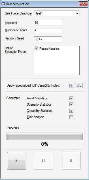
75

76 error 21 on the sample mean meaning one will arrive at a better approximation of the average performance. However, the greater the number of Iterations, the longer the total run time. If the input file has been run to produce a simulation before, the parameters from the last simulation run are saved to the input file and will automatically be loaded into the window in Figure 35. If the input file is new, the default number of Iterations is 1,000. Allowed values are integer values greater than zero and less than 32, Number of Years The run time is also dependent upon the Number of Years chosen for the simulation, as steady state performance is not achieved immediately. There are starting and ending effects due to increased asset availability at the beginning of an iteration and due to truncated scenarios at both beginning and end of an iteration that must be discarded; otherwise, they would significantly skew the asset assignment results. This is similar to the process of burn-in [30]. Empirical testing during past studies has shown that a period of one year at the start and end of each simulation is sufficient to remove all starting and ending effects. Therefore, the user must enter a total number of Years that includes two years that will automatically be discounted and removed from the statistics generation. For example, to have three full years of valid statistics generated, the user must enter five years in the input field in Figure 35. Allowed values are integer values greater than 0 and less than 50; the default value is five years Random Seed The Random Seed is used as the input to the random number generator in Tyche. By selecting a Random Seed, the user can choose to either a) hold the seed constant and vary inputs to determine the effect of the inputs under the same conditions, or b) vary the seed using the same input to determine the effect of the input distribution on the output. Doing both at the same time does not hold any value for an experimenter. The default value is -2,147; the allowed range of integer values is between -2,147,483,648 and List of Scenario Types The list of Scenario Types is also displayed in Figure 35. The user may choose to remove one or more of them from the run by simply deselecting the box beside the appropriate Scenario Types. The default value is to include all Scenario Types Apply Specialized Lift Capability Rules The Apply Specialized Lift Capability Rules checkbox in the Run window allows the user to apply specialized Lift Capability rules to the simulation run. As discussed in Section 4.2.1, specialized assignment rules can be applied to Assets that only provide Capabilities whose names start or end with the term Lift (such as Sealift or Airlift) to a mission. If selected, only the Lift Capabilities are assumed to be required at the beginning and at the end of the mission. This represents delivery and pickup of items at the start and finish of a mission. 21 For a further discussion of sample error, please refer to and Annex B. 58 DRDC CORA TM

77 Generate Statistics The user can also choose to have the Asset Statistics (.tya extension), Scenario Statistics (.tys extension), Capability Statistics (.tyc extension), and/or the Risk Analysis (.xls extension) computed by selecting the appropriate box in the Run window. Checking any of these boxes tells Tyche to compute those statistics as soon as the run is completed and the output file has been written (.tyo extension). If these boxes are not selected, then the Data Analysis Environment must be used to compute the statistics (see Section 4.5) after the fact. The Risk Analysis requires Microsoft Excel to be installed, with the corresponding version of Risk.xls file that depends on the version of Excel installed. These files are automatically installed with Tyche in the install folder, and will be copied to the same folder as the.tyi file used for conducting the simulation. However, the entire risk analysis procedure has not yet been fully automated within Tyche. At this time, the Excel file must be tailored specifically to the simulation input data; otherwise, the Risk Analysis will fail. For more detailed information on the Risk Analysis and how to set up the file, refer to Annex B. If all of the previous conditions are not met, the Risk Analysis is skipped Run buttons A run using the parameters as displayed in Figure 35 can be performed. Once the user presses the Run Simulation button, a window will be displayed proposing a folder name and an input file name: the folder name will be given to the name of the folder where the files will be saved. Since Tyche creates many different files for the same input (one input file, one output file, and up to four Data Analysis files, as discussed), the creation of a single folder for all simplifies the management of these files. The input file is then re-saved in this folder to ensure an unadulterated copy of the input data is available with the output data. It is recommended that the user accept the default names and press the Save button. During the run, Tyche will create an output file with the same name as the input file, but with the extension.tyo. The progress bar at the bottom of the Run Simulation window will show the percentage of completed iterations as time progresses. The Pause button allows the user to halt the simulation currently in progress (freeing up CPU resources to perform another task), and resume when the Start button is pressed (once the user wishes to continue the simulation where they left off). The Stop button terminates a simulation (in case of an error, for restarting debugging, to free up resources, to shut down one s computer, etc.); when the Stop button is used in the GUI, the simulation cannot be resumed from where it left off and must be re-started from the beginning. After terminating a simulation, the input file and a partial output file will exist in the save folder location, allowing the user to view the results up until the last completed iteration that was run Running a Monte Carlo discrete event simulation (MCDES) At its core, Tyche is a scheduling program that runs a MCDES (through the Tyche Simulation Engine). The user specifies the total number of iterations, as well as the number of years simulated per iteration for the Monte Carlo [31] portion of the simulation. For the discrete event implementation for each iteration [32], Asset data are first initialized. A list of events is then generated from both the Scenarios, as well as specific Asset Levels, to become the demand function for Assets. The best available Assets are assigned to the events (refer to subsection DRDC CORA TM

78 for detail on the function of events). The output is then written to a file and the process repeats. Figure 36 illustrates the various steps executed by the Tyche SE for a single iteration. Initialize Assets Data Create List of Events Assign Assets to Events Output Data to File Figure 36: Illustration of the list of steps followed for any given iteration. The following subsections describe each step of Figure 36 and the programmatic logic in more detail. Such description is not required for a user guide but was added to help analysts (advanced users) obtain a thorough understanding of Tyche processes and outputs. In particular, an analyst operating Tyche would need to know what statistical distribution is used when creating the list of events and how Tyche selects Assets for each event. The reader who does not need such details may skip the following subsections and go directly to Section 4.4 for the OpSched Environment Simulation initialization At the beginning of the simulation run, Tyche creates an instantiation of all Assets of the selected Force Structure for the run. As mentioned in Section 4.2.5, Assets have four fixed attributes: a name, an Asset Type, a home Base, and a scheduling offset. In addition, it also possesses two dynamic lists: a Level History List and a Future Event List. The Level History List keeps track of previous Levels associated with the Asset, as well as the corresponding starting and ending dates. The Future Event List temporarily stores the list of events to which the Asset is pre-assigned. The Future Event List is important since the Level History List is built from it. At the beginning of each iteration, the Assets have their History Level List and Future Event List emptied. These two lists are populated during each iteration. For each iteration, a single list of all events will be generated with no Assets assigned. On the day an event occurs, Tyche will then search to assign the best group of Assets for this event. Functionally, once an Asset is assigned to a particular event, then this event is added in the Future Event List of this Asset. It is called the Future Event List because the Asset will not be dedicated to this event right away. In general, the Asset is likely already occupied with some other activities and will require some preparation time to get ready for the new assigned event. On the day the Asset will formally take part in the activities associated with the event, the event will be removed from the Future Event List and a corresponding Level History List element will be created Creation of a discrete list of events An event occurs every time a mission begins or an Asset changes Levels. A Source, Cause, Location, Start Date, and Duration are associated with each event. The Source of an event is the initial trigger for asset assignment, which can be either an Asset or a Scenario. Because Assets can have multiple Levels and Scenarios can 60 DRDC CORA TM

79 have multiple Phases, the Cause of the event must also be identified. For example, if a specific Asset required maintenance, with Maintenance being one Level of that Asset, then the Maintenance will be requested by an event that has the Asset as the Source and the Maintenance Level as the Cause. Tyche treats events having an Asset as Source differently from those having a Scenario as Source. In the former case, the event will only occur if its associated Asset (the Source) is available or can be bumped to the requested Level (the Cause). In the latter case, the event will occur regardless of the availability of any Assets. The Location of an event is either a Base or a Theatre. More specifically, if the Source is an Asset then the location is the Base of that Asset. If the Source is a Scenario, the location is determined randomly using the list of possible Theatres for the Scenario and their associated probabilities (see Section ). The Start Date and Duration specify, respectively, the date the event starts and the number of days it will last. The duration is determined by using a triangular distribution built from the minimum, most likely (mode) and maximum durations associated with the Cause of the event (see Sections and where the durations were entered). The determination of the start date is more complex and is best understood through a discussion of the full list of events. To build the list of events, Tyche first selects a random value that is used as an offset from day 0 for all scheduled events. This effectively shifts time window for the simulation such that the portion of the schedule that is fixed will be randomized for each iteration (i.e., start of simulation t=0 for the simulation will not always align with day 0, or January 1). This is illustrated in Figure 37, with the time window shown as the shaded yellow portion of the schedule on a list of events (random in blue, scheduled in orange), and the scheduled (pink/orange) events offset with respect to day 0. Random Schedule Offset Scenario Phase Offset Day 0 t=0 Figure 37: Selected time window for events. The time window for the iteration is thus from the initial random date until initial random date + [ number of years simulated * 365 days/year], where the number of years simulated is DRDC CORA TM

80 specified by the user in the Run window (see Section 4.3). 22 Once a time window has been specified, the events expected to occur during this time interval are generated and stored chronologically in a list. Events that start on the same date are listed in the order generated, and all events are processed one at a time. The number of Events generated and their Start Dates depend on the Cause of these events. If the Cause is either a Scheduled Level (Source is Asset) or Scheduled Phase (Source is Scenario), Tyche creates an event every time this Cause is scheduled inside an iteration s selected time window. More specifically, if the Start Date (or Start Date + Offset if the Source is an Asset) of the Scheduled Cause is x and its frequency f, then the Scheduled Cause will occur every day given by: x + [n365/f] where n (where is the set of all integers). All such Scheduled Causes that fall inside the selected time window will be added to the list of events. Note that the duration of the events that overlaps with the beginning or the end of the time window will be truncated to fit completely inside the time window, as shown in Figure 37. Also, events that are too short to have any Assets assigned (Based on minimum preparation and travel time) are removed from the simulation. As a result, the first and last year of all simulation iterations are not counted in the statistics generation to eliminate this burn-in effect. If the Cause is a Random Level or Random Phase, then the number of events falling in the time window is determined from a Poisson distribution since the events are assumed to be independent of one another 23. Explicitly, for a time window of n years and a Random Cause, which has a frequency of occurrence per year, the number of events, N, is determined by selecting a random number, r, uniformly distributed on [0,1], and applying Equation (7) to rescale the probability. Equation (7) determines the number of events, N, to be equal to i only when the conditions are satisfied for r; i is evaluated from 0,1,2,3, until the limit of the upper constraint is reached at ( * n )*2 *n (or at least 1 event, whichever is greater). The Start Date of each of Random event is randomly selected from the set of days inside the time window using a uniform distribution. N i where i1 ( n) ( n) iz exp( n) r exp( n) (7) j0 j! j i j0 j! j NOTE that the sum over the integer j from 0 to i-1 is set to 0 in the case i=0. The events corresponding to Levels or Phases that are of the follow-on type are treated differently. For follow-on Phases, one event is created every time there is an event generated by the Phase that they follow. Thus the preceding Phase determines the start date for the follow-on ones. For follow-on Levels, no associated events are generated until the Asset (the Source) goes to the Level that precedes the follow-on Level. 22 Noting that Tyche does not take leap years into account. 23 In reality, the geo-political situation is a complex set of inherently interconnected events. However, under the assumption that no knowledge can be obtained about where or when such events might be predicted to happen in a Monte Carlo simulation, the events can be considered independent from one another. 62 DRDC CORA TM

81 Assigning and registering Assets to events Once a list of events for the iteration (k) has been built, Tyche will assign Assets to each event (l) in a chronological order. However, first each Asset is set at its default Level. Then, starting with the earliest event, Tyche assigns Assets to each event (the specific assignment algorithm will be discussed in the following sub-section). The flow chart in Figure 38 illustrates how Tyche processes each simulation run with respect to the list of events. When dealing with a new event l, Tyche first determines whether or not the Source of the event is a Scenario or an Asset. In the former case, Tyche assigns Assets to the event. In the latter case, Tyche determines whether or not the Asset (the Source) is currently at the default Level. If the Asset is at the default Level, then Tyche assigns the Asset to the event. If the Asset is not at the default Level, then Tyche determines whether or not the Asset can be bumped from its current activity (the Asset can be bumped if the bump rank of the current Level is less than or equal to the one of the Cause of the event refer to section 4.2.4) and reschedule the current activity to a later date. If the Asset can be bumped, then Tyche assigns Assets to the event. The event that the Asset was bumped from is evaluated to determine if the remaining time in the current activity (Level) should be re-scheduled. The new event is re-scheduled depending on the re-schedule instruction specified in the bump data associated with the current Level of the Asset (see Section ). If the Asset cannot be bumped from its current activity, then Tyche verifies whether or not the new event should be re-scheduled. The new event is re-scheduled depending on the re-schedule instruction specified in the bump data associated with the Level corresponding to the Cause of the event. If the event is re-scheduled, the start date is set to the day the Source of the event is ending its current activity. Once an event has been processed, the event list is checked to see if new events have been added. If all events have been processed, the next iteration can begin. If all iterations have been processed, the simulation is complete, and the data analysis can begin. DRDC CORA TM

82 k th Iteration Start date, sample frequency and duration l th Event Is source Scenario? Yes No Is source available? Yes No Can source activity be rescheduled? Assign assets through capability matching Yes No Should J th event be rescheduled? Yes No Reschedule current activity for source, if necessary Reschedule event for when the current activity ends No assets are assigned to event No All events processed? Yes No All iterations processed? Yes End simulation Figure 38: Flow chart describing the logic used by Tyche. 64 DRDC CORA TM

83

84 corresponds to selecting a matching on the graph. Every Asset for which at least one Capability Supply in a link pertaining to the matching belongs to the group of selected Assets. As noted above, only the Capability Cost and Timeliness Score can be assigned as a weight associated with the links in a bipartite matching. This is possible because these two scores are given as a sum over the Capability Demands that are matched (see Equations (2) through (5)). The Excess Score and Conflict Score cannot be obtained through a distributed sum along the links pertaining to the matching. Thus, if the Excess Score and Conflict Score do not belong to the selected Scoring Criteria then the optimal matching corresponds directly to the highest weight matching, which is a well-known problem in graph theory [33]. In particular, the Backtracking and Backjumping algorithm has been applied successfully to this type of problem [34]. Because the weights for the excess and conflict Scoring Criteria are typically small, this algorithm produces solutions that are near-optimal and efficient to compute. The Backtracking and Backjumping algorithm was thus selected as the assignment algorithm for Tyche Version 2.0 and onwards. In more detail, the algorithm used by Tyche 3.0 follows these steps: 1. Create nodes for every Capability Demand and Capability Supply of the event s Source. Note that if there is a Capability Demand requiring, for example, three Interdiction Capabilities at a level of 0.8, then three nodes are created each requiring Interdiction Capability at a level of 0.8. The Capability Demand from the event is the first layer of capability that must be matched. 2. Store all the Capability Demands into a dynamic list that will keep track of the Capability Demands met. 3. Create nodes for every Capability Supply and Capability Demand of all Assets that belong to the Search Domain associated with the event s Cause. 4. Store these available Assets in a dynamic list. Note that the available Assets are filtered to remove infeasible solutions (i.e., those Assets that cannot be bumped to the necessary Level, those Assets that cannot make it to Theatre before the timeliness threshold, and those Assets that have Level and Multi-Level Constraints that would prohibit their use). 5. Add links between corresponding Capability Demands of the event s Source and Capability supplies of available Assets. 6. Using the Scoring Criteria of the event s Cause (see section ), calculate the score for each available Asset using Eq. (1). Select the Asset with the highest score. If no Asset has a positive score, no Assets are selected. 7. If there is a selected Asset, remove all the Capability Demands met by the selected Asset from the list of Capability Demands and select the links corresponding to these matched Capabilities. 8. If there is a selected Asset, remove the selected Asset from the list of available Assets. 66 DRDC CORA TM

85 9. Repeat steps 6, 7 and 8 as long as the overall score across all assigned Assets increases (unless all available Assets have been selected or have been exhausted). Note that every time step 6 is repeated the incremental score for each individual Asset tends to decrease since the only positive components to the score is the Capability score (see Section ) and this score decreases as less and less Capabilities are left in the list of Capability Demands (the matched Capability Demands are removed in step 7). 10. If the Source of the event is a Scenario and the first layer of Capability Demand is being evaluated, verify that the group of selected Assets meets the various Scoring Criteria thresholds. If one or more of the thresholds are not met, remove the selected Assets for the event and retry the layer. 11. Verify if Essential Capabilities are left unmatched. If so, then unselect every Asset (the selected Assets are unsuitable) and exit the algorithm. No Assets are assigned to the event. 12. Move to the second layer and look for Assets to meet the Capability Demands of the Assets selected at the first layer (the Asset Capability Demand of those Assets already matched to the event). If no Assets were selected at the previous layer, go to step For all Assets selected at the previous layer, repeat these steps: a. Looking at all previously selected Assets, investigate whether or not any of these Assets belong to the Search Domain of one Asset selected at the previous layer and can meet some of its Capability Demands. In terms of the graph, this operation corresponds to looking for additional possible matches before adding new nodes to the graph. b. Remove Capability Demands met from the Capability Demand list. c. Add nodes for every Capability Demand and Capability Supply for Assets pertaining to this Asset s Search Domain if nodes for this Asset have not already been added. d. Store these available Assets in a dynamic list. e. Add links between corresponding Capability Demands of the event s Source and Capability supplies of available Assets. f. Using the Scoring Criteria of the event s Cause, calculate the score for each available Asset. Select the Asset with the highest score (zero and negative scores are not allowed). g. Remove all the Capability Demands met by the selected Asset from the list of Capability Demands and select the links corresponding to these matched capabilities as part of the optimal matching. h. Remove the selected Asset from the list of available Assets. i. Repeat steps f, g, and h as long as the overall score increases. DRDC CORA TM

86 j. Verify whether or not essential Capabilities are left unmatched. If so, then remove all the nodes and links that were added at this layer. Remove also the Asset for which the Capability Demand cannot be met and backtrack to the previous layer to look for a different set of Assets to select at this previous layer. k. Check for redundancy. More explicitly, check whether or not a newly selected Asset could have entirely provided the Capability supplies provided by a previously selected Asset at a higher layer. If there is such redundancy, then replace the redundant Asset by the newly selected Asset and backjump at the layer where the redundant Asset was selected. Remove all the nodes and links that were created after that layer and restart assigning Assets from this previous layer. 14. Go to step 12 until all Capability Demand matched at all layers, no feasible solution can be found, or the number of tries at each layer exceeds 32,000 (hard coded value). 15. Verify that all Assets are waiting for those which are essential to their Capability Demand matching (departure dates to Theatre must match for dependent demand chains). The algorithm may appear complex, but the basic concepts are very simple. The selection of Assets is done in a multi-layered way. At each layer, Assets are selected to meet the Capability Demands that were introduced at the previous layer. If at some layer the Capability Demands cannot be met (illustrated by the unmet Demand b in Asset 2 on the left in Figure 40), then the algorithm backtracks to the previous layer and selects a different group of Assets from what had previously been selected. At each layer, after a group of Assets has been selected, the algorithm checks for redundancy. If redundant Assets are found (Asset 3 in Figure 40), then the redundant Asset is removed and replaced by the new Asset (Asset 2 in Figure 40) that can provide the Capability that the redundant Asset was providing and the algorithm backjumps to the layer where the redundant Asset was selected. 2 1 Figure 40: Illustration of the backtracking (left) and backjumping (right) processes. If at some layer, Essential Capabilities cannot be met, then backtracking is required in order to step back to a previous layer and look for a different group of Assets to select. The need for backjumping is not quite so evident. Consider a mission occurring 1,000 nm from the Halifax naval base that requires some Capabilities provided by a Frigate and some provided by a 1 2 C 3 68 DRDC CORA TM

87 Helicopter. Assume that there are Frigates available in Halifax and Victoria; and no more Helicopters are available at Halifax, but some are available in Victoria. It is also assumed that the Helicopter requires Air Support Capability to be provided by a Frigate from the same Base. In this situation, the algorithm will select at the first layer a frigate from Halifax and a Helicopter from Victoria (the Frigate from Halifax will have a better score than one from Victoria since it is closer to the Theatre and will provide a more timely response to the mission). At the second layer, a frigate from Victoria will be selected to provide Air Support to the helicopter. Then the algorithm will look for redundancy and will observe that the second Frigate could have provided all the capabilities that the first selected Frigate was providing. The algorithm will then replace the Halifax-based Frigate by the Victoria-based Frigate and backjump to the first layer. The selected Assets from this first layer are now a Frigate and Helicopter both from Victoria. Proceeding to the second layer, the algorithm will match the Air Support Capability required by the Helicopter with the Frigate from Victoria and no additional ships are needed. Without the backjumping process, the algorithm will have ended with three selected Assets (two Frigates and one Helicopter) Run output to a.tyo file After Assets have been assigned to all the events occurring in the time frame of a given iteration, Tyche stores results from the run in a text-based output file (*.tyo). More precisely, details about the Cause, Source, selected Assets, and any Capabilities that are not met for an event are written on a line for each event (see Table 3 for an example output). This output file is used with the OpSched Viewer (Section 4.4) and Data Analysis (Section 4.5) environments, whose role and use in Tyche are described in the two subsequent sections. An important note about performing output operations in Tyche is that the output file generated from a simulation run is innately tied to the input file (*.tyi) from which the output file was generated. The file path of the original input file is written in the output file. DRDC CORA TM

88 Table 3: Sample partial simulation output file, formatted in columns for easier viewing. EVENTS: Source Type (String) Source Name (String) Cause Name (String) Start Date (Integer) End Date (Integer) Location (String) Rescheduled Activity (Boolean) [For each asset assigned to the event: Asset Name (String) Level Name (String) Scenario Sc9 Sanction Location1 FALSE Multi-Purpose Ship 5 Deployed FALSE Scenario Sc9 Sanction Location1 FALSE Multi-Purpose Ship 8 Deployed FALSE Scenario Sc9 Intervention Location1 FALSE BattleGroup 15 Deployed FALSE Asset Multi-Purpose Ship 6 Not Used Halifax FALSE Multi-Purpose Ship 6 Not Used FALSE Asset Multi-Purpose Ship 7 Not Used Halifax FALSE Multi-Purpose Ship 7 Not Used FALSE Scenario Sc9 Intervention Location1 FALSE BattleGroup 16 Deployed FALSE Asset Multi-Purpose Ship 8 Not Used Halifax FALSE Multi-Purpose Ship 8 Not Used FALSE Asset Multi-Purpose Ship 10 Not Used Victoria FALSE Multi-Purpose Ship 10 Not Used FALSE Asset JSS 3 Not Used Victoria FALSE JSS 3 Not Used FALSE Asset BattleGroup 15 Not Used Halifax FALSE BattleGroup 15 Not Used FALSE Asset Multi-Purpose Ship 5 Not Used Halifax FALSE Multi-Purpose Ship 5 Not Used FALSE Asset JSS 1 Not Used Halifax FALSE JSS 1 Not Used FALSE Asset JSS 1 Maintenance Halifax TRUE JSS 1 Maintenance FALSE Asset Multi-Purpose Ship 5 Maintenance Halifax TRUE Multi-Purpose Ship 5 Maintenance FALSE Asset JSS 3 Maintenance Victoria FALSE JSS 3 Maintenance FALSE Asset Multi-Purpose Ship 6 Maintenance Halifax FALSE Multi-Purpose Ship 6 Maintenance FALSE Asset Multi-Purpose Ship 10 Maintenance Victoria FALSE Multi-Purpose Ship 10 Maintenance FALSE Asset JSS 1 Not Used Halifax FALSE JSS 1 Not Used FALSE Asset Multi-Purpose Ship 5 Not Used Halifax FALSE Multi-Purpose Ship 5 Not Used FALSE Asset JSS 3 Not Used Victoria FALSE JSS 3 Not Used FALSE Asset JSS 2 Maintenance Halifax FALSE JSS 2 Maintenance FALSE Asset Multi-Purpose Ship 7 Maintenance Halifax FALSE Multi-Purpose Ship 7 Maintenance FALSE Asset Multi-Purpose Ship 6 Not Used Halifax FALSE Multi-Purpose Ship 6 Not Used FALSE Asset Multi-Purpose Ship 11 Maintenance Victoria FALSE Multi-Purpose Ship 11 Maintenance FALSE Asset Multi-Purpose Ship 10 Not Used Victoria FALSE Multi-Purpose Ship 10 Not Used FALSE Base Departure Date (Integer) Theatre Arrival Date (Integer) Theatre Departure Date (Integer) Base Arrival Date (Integer) Was Bumped (Boolean)] Headers specify the contents of each column and each line in the table is dedicated to a single event. The last seven columns shown here are repeated for all Assets assigned to the event (not shown here). Any Capabilities missing from the event are listed immediately afterwards. 70 DRDC CORA TM

89

90 segments. When the timeline is scaled, the axes for both panes will update together, maintaining a seamless look between the schedules. Along the horizontal axis for the left pane (at the top) are the names of the Assets, with their home Bases, in the order in which they were entered in the Force Structure that was selected in the simulation. If the Names and Base names are more than 24 characters long, they are partly truncated. This pane can display the OpSched of up to 39 Assets simultaneously. If the Force Structure is composed of more than 39 Assets, then a scroll bar will appear in the bottom of the panel to scroll between the various Assets, as seen in next subsection. Each column of text and coloured bars corresponds to one Asset. For each Asset listed above the pane, the colored bars represent the history of Levels corresponding to the Asset throughout the entire simulation time,24 such as operational levels and maintenance. Up to 10 different colours are automatically cycled through for each Level; however they can be changed by the user (more information on color schemes is available in Section 4.4.4). The right pane displays the missions (occurrence of Scenario Phases in space and time), colourcoded by Scenario Type, by default. These events are compressed into as small schedule as possible, showing overlapping events as new columns (non-overlapping events are added to existing columns wherever space is available). As a result, a finer resolution or a different color scheme may be required to determine when one event ends and another begins Asset OpSched pane The Asset OpSched pane displays the details of the simulation output, interpreted graphically so that the user can see how the state (Level) of each Asset changes over time. Each colored bar represents a Level for the Asset, which may correspond to an Asset-driven event (scheduled, random, or follow-on) or a Scenario Phase (on-demand) Level. The start and end of each bar corresponds to the start and end of the asset assignment to the event not necessarily the actual start or end of the event itself. This will take into account all of the timing considerations described in Section The one exception to this is the bump time. When an Asset is being bumped from one Level to another, the time does not display on the OpSched Viewer. This is a known flaw of the Tyche GUI that needs to be addressed in the next build. This bump time will not display any differently that the background black color; however the user will be able to find instances of it in several ways. By placing the mouse cursor over a coloured area (on either the left or right pane), then pressing and holding the right mouse button, the OpSched Viewer will display additional information about the item on which the right-click has occurred. This is very useful for learning precisely what a given Asset was doing at any given point in time. For areas in the OpSched with no data, either outside the Asset column area or during bump time, no data will be displayed on rightclick. 24 Note that the one year of data at the start and end of each simulation that is removed for data analysis purposes is shown here. This is to maintain the integrity of the output file, for debugging purposes, and to allow the user to complete additional analyses on the data, should they choose to parse it in another program. 72 DRDC CORA TM

91 Figure 42 shows an example of the information displayed when right-clicking on a coloured bar (the first blue rectangle in the JSS 1 column in Figure 41) in the left pane. The name of the Asset appears in the header of the information window. Below the header, two blocks of data are provided. The first one provides information about the Asset: Asset s current Level Name, Base Departure Date, Theatre Arrival Date, Theatre Departure Date, Base Arrival Date, and Rescheduled parameter value (specifies if the Asset was rescheduled to participate in this activity, either Yes or No). The second block of data provides information on the event to which the Asset was currently assigned: Event Source, Event Cause, Start Date, End Date, Location, and Rescheduled parameter value (specifies if this event was a rescheduled activity, either Yes or No). Figure 42: Asset OpSched Viewer information displayed on right-click Mission OpSched pane The Mission OpSched pane displays the Scenario Phase events as they occur in distributed space and time. Just as for the Asset OpSched pane, each colored bar represents an event corresponding DRDC CORA TM

92 to one Scenario Phase. The start and end of each bar corresponds to the start and end of the event not the asset assignment to the event itself. By placing the mouse cursor over a coloured area, then pressing and holding the right mouse button, the OpSched Viewer will display additional information about the item on which the right-click has occurred. However, here the data is tailored to Scenario Phases, including: Scenario, Phase, Start Date, End Date, Theatre, and Rescheduled parameter value. Figure 43: Mission OpSched Viewer information displayed on right-click Alternate colour schemes The Edit Asset Colours button, located to the left of the list of Assets, allows the user to change the colouring of Assets in the left pane. Figure 44 displays the Edit Asset Colours window. To view the colour of an Asset s Level, the user selects that Asset in the list entitled Assets. The Asset s Levels will be displayed in the second list. Upon selection of the Level of interest in the list entitled Levels, the colour of that Level for this Asset will be displayed in the Sample picture box. To change the colour, the user presses the Change button, and a window will be displayed for the user to choose a colour for this Level of the Asset. Once all colour viewing or changing is completed for the Assets, the user presses the OK button in the top-right corner of the Edit Asset Colours window. The viewing and changing of the colours in the Scenario (right) pane functions similarly to that of the Asset colours. There are two ways to view the colours though by Scenario Type or by Scenario. There are two radio buttons labelled Colour by Scenario Type and Colour by 74 DRDC CORA TM

93 Scenario, which allow the user to change the colouring of Scenario Types and Scenario Phases, respectively. These buttons are located just above the right Mission OpSched pane. The Scenarios are coloured by Scenario Type by default, so selecting either of the Edit Scenario/Scenario Type Colours radio buttons will open an editing window with the Scenario Types in the list labelled Scenario Types. The colour associated with a selected Scenario Type will be displayed in the Sample picture box. To change the colour, the user presses the Change button, and a window will be displayed for the user to choose a colour for this Scenario Type. Figure 45 displays the Scenario Type colouration and colour palette window. Once all colour viewing or changing is completed for the Assets, the user presses the OK button in the top-right corner of the Edit Scenario Type Colours window. The same can be done for individual Scenarios and Phases when the Colour By Scenario radio button is selected. Changes made to the colour scheme of either the Assets (or the missions) will be immediately reflected in the OpSched Viewer upon closing the Edit Colour window. They will apply to all iterations viewed, but will not be remembered when a new output file is opened. Figure 44: Asset Level colouration window. DRDC CORA TM

94 Figure 45: Scenario Type colouration window Alternate background color The user may also toggle the default Level colour for all Assets in the left pane from black to white by clicking the Toggle Default Level Colours button at the bottom left corner of the left pane in the OpSched viewer. Figure 46 shows the OpSched viewer with the default Level colour as white for each of the Asset columns. 76 DRDC CORA TM

95 Figure 46: OpSched Viewer with white Asset background Viewing Iterations By default, upon opening an output file, the OpSched Viewer will display information from the first iteration in the file. The user may change the iteration by using the controls in the upper-right corner of the OpSched window. In the frame entitled Iteration, the text field displays the current iteration that is being viewed. The value may be overwritten with any desired specific iteration number. Alternatively, the user may press the Up or Down arrows to view the previous or next iteration, respectively. Figure 47 shows the OpSched for the second iteration of a simulation. DRDC CORA TM

96 Figure 47: Second iteration of tutorial data displayed in the OpSched Viewer. In the top-right corner of the OpSched viewer, next to the Iteration frame, is a frame entitled Interval. The Start Date and End Date refer to the inclusive bounds of the time frame that is currently visible in the two panes of the OpSched Viewer. The user may manually change these values to view a specific interval. The OpSched Viewer may then change the values entered to ensure that the exposed interval is a multiple of ten so that it may be split into ten equal integer portions. Next to the Interval is the Zoom Throttle. This frame contains controls that allow the user to zoom in and out. This is useful to see precisely which day particular events begin and end. By default, the view is zoomed out as much as possible to allow the user to view the entire iteration at a glance. The Zoom In and Zoom Out buttons will zoom in on or out from the current centre of the exposed interval, growing or shrinking the interval by the number of days selected on the Zoom Throttle. The Zoom Throttle may be changed to zoom by more or less days as desired. When zooming, half the number of days shown on the zoom throttle will be adjusted on the top of the interval, and the other half from the bottom. For example, if the exposed interval is from 0 to 360 days, and the throttle is set to 80, if the user presses the Zoom In button, the new interval would be 40 to 320 days. 78 DRDC CORA TM

97 Finally, by left-clicking on either of the panels, the OpSched Viewer will attempt to zoom in on the click region by the number of days set by the Zoom Throttle. Thus, it will first centre the viewed interval on the area that was clicked, and then proceed to zoom in on that area Search Function Tyche output files can be extremely large (often greater than 256 MB) and, as a result, are slow or impossible to open using conventional text editors. However, the user may need to search through the output using keywords to identify specific events, Scenarios, Assets, or Capabilities. For example, a user may want to determine why no Assets are being assigned to a given Scenario. By searching for this event in the output, the user can determine if other events occurring at the same time may be interfering with asset assignment. The OpSched Viewer is meant as a graphical representation of the output and does not allow the user to search the output directly. A complex search function, built upon the idea of a "Find" function (commonly available in Notepad or WordPad ) for multiple strings is implemented to search the output directly. The search criteria are tailored to the Tyche output and constructed as a set of embedded controls in the OpSched Viewer shown in the bottom right corner of Figure 42. The criteria are constructed of common combinations of data that a user could use for debugging or analysis purposes. The search function looks for all instances in the Tyche output (.tyo) file, where all requested data are listed for the same event (on one line of the output file). Data in these strings are used to determine if the search criteria have been met. The.tyo output file has the following format for events in a simulation: Asset;Asset Name;Level;Start Date;End Date;Base;Rescheduled Event;Assigned Asset Name;Level;Base Departure Date;Theatre Arrival Date;Theatre Departure Date;Base Arrival Date;Asset Was Bumped;Number of Capabilities Missing at Required Level;Capability Names (if any);number of Capabilities Missing at Marginal Level;Capability Names (if any) Or: Scenario;Name;Phase;Start Date;End Date;Theatre;Rescheduled Event;Assigned Asset Name;Level;Base Departure Date;Theatre Arrival Date;Theatre Departure Date;Base Arrival Date;Asset Was Bumped;Number of Capabilities Missing at Required Level;Capability Names (if any);number of Capabilities Missing at Marginal Level;Capability Names (if any) where the first item (delimited by semi-colons) is the Cause of the event (either Asset or Scenario), and the second item is the event Source (i.e., the name of the Asset or Scenario and the name or the corresponding Level or Phase). The next four elements are ignored for the search. Then the list of assigned Assets can be used to help filter the search; the assigned Asset name and the next six data elements are repeated for each assigned Asset to an event. The Capabilities missing at the required and marginal Levels are not used in the search function. To structure one s search, the following subsections will lead the user through the fields in the search function, as shown in Figure 48. DRDC CORA TM

98 Sanction

99 Table 4: OpSched search functionality. Option Selected Rule Applied Search Results All Check Data boxes off. All Check Data on. All Number of Occurrences = 0. Check Data for one or more (but less than total) Asset Types on. Number of Occurrences = 0. Check Data for one or more (but less than total) Asset Types on. Number of Occurrences > 0. No specific matching requirements are set. Find events that contain exactly zero of each and every Asset Type. Find events that contain exactly zero of each checked Asset Type. Find events that contain exactly the number specified of each checked Asset Type. Table 5: OpSched searches in tutorial example. All events. Events where no Assets are assigned. Events where none of the specified Asset Types are assigned. Events where the exact number of the specified Assets Types are assigned. Option Selected All Check Data boxes off. All Check Data on. All Number of Occurrences = 0. Check Data for Battle Group on. Number of Occurrences = 0. Check Data for AAW Module on. Number of AAW Module Occurrences = 1. Number of Search Results Example Event String 40 (1);Scenario;Sc9;Sanction;24;204;Location1;False; Multi- Purpose Ship 5;Deployed;29;36;204;211;False;Multi- Purpose Ship 6;Deployed;29;36;204;211;False;Multi- Purpose Ship 7;Deployed;29;36;204;211;False;JSS 1; Deployed; 29;36;204;211;False;AAW Module 13; Deployed;29;36;204;211;False;;0;0 2 (1);Scenario;Sc9;Sanction;866;1046;Location1;False;;3; Interdiction;Interdiction;Interdiction;3;Interdiction; Interdiction;Interdiction 22 (2);Scenario;Sc9;Sanction;127;307;Location1;False;Multi- Purpose Ship 8;Deployed;132;143;307;318;False;Multi- Purpose Ship 9;Deployed;132;143;307;318;False;Multi- Purpose Ship 10;Deployed;132;143;307;318;False;JSS 3; Deployed;132;143;307;318;False;AAW Module 14; Deployed;132;143;307;318;False;;0;0 38 (3);Scenario;Sc9;Intervention;184;544;Location1;False;Batt legroup 15;Deployed;217;218;364;365;False;Multi-Purpose Ship 5;Deployed;217;218;364;365; False;JSS 1;Deployed;217;218;364;365;False;AAW Module 13;Deployed;217;218;544;545;False;;0;0 DRDC CORA TM

100 Search buttons There are two main buttons that start and stop the search, (number 2 in Figure 48). The Find button starts a search once the search criteria have been entered.. Once initiated, the search looks for all matching instances of the search criteria in the.tyo file on a line-by-line basis. To make sure that search results are available to the user as soon as results are found (as the full search may take some time on large output files), the search function automatically updates the tree view (pane 3 in Figure 48) containing the search results. When a search is running, it can be stopped by pressing the Stop button Search results display When the search is running (or complete) and results are found, they are automatically displayed in the search results pane (3 in Figure 48). Each item found is displayed in a tree view, grouped under its corresponding Iteration parent node for easier navigation. When the user clicks on a search item found, the OpSched Viewer will automatically update its view to display the appropriate iteration in the graphical representation above the search, with each search result numbered in brackets under the expanded node. Each search result contains the line containing the matching strings taken directly from the Tyche output file, using the format shown on page 79. The total number of matches resulting from the search will be displayed in numerical format following the Search Results title for the pane. For instance, if the user selects the JSS from the tutorial example at a Maintenance Level, the search function will return all events where the JSS goes through a Maintenance Level. There are 51 matches found in the.tyo file that the user can then view in the Search Results tree, which fills the pane labelled number 3 in Figure 48, and is shown with one iteration node expanded in Figure 49. Figure 49: Operational Schedule Viewer search function after a search has been run Save search results to file Once the search has completed or has been stopped by the user, the results can be exported to a text file using the Save button (4 in Figure 48). Tyche, by default, attempts to save the search results to a file named OpSchedSearchResults.txt by prompting the user with a Save As dialog box. Using this dialog, the user can choose any destination and/or file name to save the search 82 DRDC CORA TM

101 results to. Aside from the search results, the file also contains useful information such as title, date and time of the search performed. Figure 50: Sample search text results. 4.5 Data Analysis environment Performing a statistical analysis on an output file generated from the running of a Tyche simulation can be done automatically following the simulation run, or anytime afterward at the user s leisure. To perform the data analysis immediately after a run (when in debug mode), the user checks the Asset Statistics, Scenario Statistics, Capability Statistics, and/or Risk Analysis checkboxes on the Run window before starting the simulation, as shown in Figure 51. If the simulation is run through the Tyche SM, all analyses are automatically conducted Note that if WinZip 9.0 (or later) with the Command Line Support Add-On is also installed, the SE will also attempt to zip the.tyo output file. If the zip is successful, the.tyo file is subsequently deleted to save space. DRDC CORA TM

102 Figure 51: Options to automatically run statistical analyses. Alternatively, any time after a run has been performed, the user may press the Analysis button on the parent window (Figure 3), select the output file from which the statistics are to be derived, in addition to the statistics that are to be calculated, and press the OK button. Figure 52 illustrates the Data Analysis window immediately after the Analysis button on the main Tyche window has been pressed. To perform the Data Analysis, the user needs to enter the name of the output file in the top text box on the Data Analysis window, check the appropriate boxes corresponding to the desired statistics and press the OK button. Three types of statistics can be calculated: Asset, Scenario, or Capability statistics. The Risk Analysis can also be computed. These four types of calculations will be discussed in detail in the following sub-sections. As the analyses are progressing, the bar will display how much of the analysis has been completed. Below the progress bar is the corresponding percentage of work completed. 84 DRDC CORA TM

103 Figure 52: Data Analysis Environment window Asset statistics Asset statistics are defined as the average number of days per year each Asset in the simulation was at each of its Levels. This is calculated by counting, for each iteration, the number of days each Asset was at each of its Levels, dividing that sum by the number of years in an iteration and then computing the average of this number over all iterations. The standard deviation of the average time spent at each Level is also calculated. 26 These data can be useful in determining whether particular Assets are being over-utilized or under-utilized, which is useful to help determine how efficient a particular Force Structure is, given the particular set of Scenarios used in the simulation. When performing the asset statistics from an output file named tutorial1.tyo, the results of the asset statistics will be stored in a file called tutorial1 Asset Stats.tya. This output file can be opened later with Microsoft Excel to build a graphical representation of the output. Using the main example used throughout this report, the asset statistics graph shown in Figure 53 was produced. The list of Assets is displayed along the front axis, the list of Levels along the side axis and the number of days per year along the vertical axis. The contents of the tutorial example output files can be found in Annex D. 26 As a reminder to the user, the Tyche output file is available for additional analysis, should they require more detail or tailoring to a specific application than what is available through the statistics that are computed automatically. The text file can be parsed easily using the format shown in page 77. To date, a number of Visual Basic for Applications macros have been written for Microsoft Excel for precisely this application; these files can be obtained from the author. DRDC CORA TM

104 Days Per Year JSS 1 JSS 2 JSS 3 JSS 4 Multi-Purpose Ship 5 Multi-Purpose Ship 6 Multi-Purpose Ship 7 Multi-Purpose Ship 8 Multi-Purpose Ship 9 Assets Multi-Purpose Ship 10 Not Used Deployed Maintenance Multi-Purpose Ship 11 Multi-Purpose Ship 12 AAW Module 13 AAW Module 14 BattleGroup 15 BattleGroup 16 Levels

105 Table 6: Information provided by scenario statistics. Sc9:Sanction Frequency AAW Module Battle Group JSS Multi-Purpose Ship 92.9% % Sc9: Intervention Frequency AAW Module Battle Group JSS Multi-Purpose Ship 93.8% % Capability statistics Capability statistics are defined as the relative frequency that individual Capabilities demanded by Scenario Phases were not met at the required and marginal levels noting that each individual Capability Demand is broken out based on the Capability Demand name and Quantity. For example, an Interdiction Capability requested at a given Quality, for a Quantity of three, would generate three individual Capability statistics. This is calculated by counting, for each iteration, the number of times an individual Capability Demand for a given Scenario s Phase was not met at either the required or marginal level, then dividing this count by the number of times that particular Phase occurred and finally averaging this result over all iterations. This information is useful in determining which Capabilities the chosen Force Structure may be lacking, when faced with given sets of Scenarios. Depending on the types of studies, in addition to the combinations of Force Structures and Scenarios, the results of these statistics may be utilized for decision support for future strategic planning considerations. When performing the Capability statistics from an output file named tutorial1.tyo, the results of the Capability statistics will be stored in a file called tutorial1 Capability Stats.tyc. Using the tutorial example used throughout this report, the content of the capability statistics file obtained is displayed in Table 7. As shown by this table, only the Capability Demands of the Phase are considered by the Capability statistics. The probability that the Capability Demands of the Assets participating in the Scenario are not met is not provided. The three Interdiction Capabilities appearing under the Sc9: Sanction corresponds to the Capability Demand for three units with one Interdiction Capability. Although, in this example, the same percentage appears for each Interdiction Capability, in a generic case these percentages can differ. 27 The percentage for the first Interdiction corresponds to the percentage of time that (which can be interpreted as a 27 Ordinarily, the matching process would be independent of the order of the capability demand within the same capability. Because the Capability Demand is processed in an ordered list by a computer algorithm, the matching process will always match the first capability demand in a set (when the Quantity is greater than one for the same capability) first, and so on down the list. Thus, the second Capability Demand can never be matched unless the first is already matched, and so on. In the generic case, the percentage of time that the at least one Interdiction Capability Demand is not met is greater than or equal to the percentage of time that at least two Interdiction Capability Demands are not met, which is greater than or equal to the percentage of time that all three Interdiction Capability Demands are not met. DRDC CORA TM

106 probability) there is at least one Interdiction Capability Demand not met. The second percentage is the percentage of time that there are at least two Interdiction Capability Demands not met. Finally, the number under the third Interdiction provides the percentage of time that none of the Interdiction Capability Demands are met. The final column, labelled Any Capability, always lists the percentage of time that any one Capability is not met for the Phase. Table 7: Information provided by Capability statistics. Sc9: Sanction Degree Of Quality Interdiction Interdiction Interdiction Any Capability Required 7.14% 7.14% 7.14% 7.14% Marginal 7.14% 7.14% 7.14% 7.14% Sc9: Intervention Degree Of Quality Peace Keeping Interdiction Any Capability Required 6.25% 6.25% 6.25% Marginal 6.25% 6.25% 6.25% Risk analysis The data analyses described so far focus on individual Assets, Scenarios or Capabilities. What is missing is a way of evaluating overall force structure performance for comparison purposes. This is where the risk analysis comes in. Risk is commonly defined as a function of cost, threat, and vulnerability [35], and can be used to compare relative force structure performance. Since a dollar figure cannot be attributed with this model, a more subjective assessment of the impact of failure in a mission is made to substitute for cost. The threat is the frequency of mission failure over a given interval, and the vulnerability is the likelihood of a single mission failure. Since the planning process revolves around Capability Supply and Demand, mission failure was defined to mean at least one Capability was not brought to the Scenario Phase [12]. Thus, the mean yearly risk (R) for a set of Scenario Phases is defined in Eq. (8), where the risk for a given Scenario Phase (s) is defined as the product of the impact (I s ) of Scenario Phase failure, the annual frequency of Scenario Phase occurrence (f s ), and the percentage of time the Capability Supply deployed by the scheduler is inadequate (P s ) [12]. R = I s f s P s s (8) The first factor (I s ), known as impact score, can be provided as a subjective input. This allows the risk assessment to incorporate subject matter expert judgement, often critical to balance the perceived effect of low impact-high frequency and high impact-low frequency Scenarios. When many Scenario Phases exist, it is often easier to group them into impact categories applying the same impact score to the entire category of Scenario Phases. The interested reader is referred to [19] for more information on the methodology for the design of the impact score (and the risk analysis in general). 88 DRDC CORA TM

107 The second factor (f s ) is assessed by averaging the number of times the Scenario occurs yearly across all iterations in a Tyche simulation run. The third and final factor (P s ) is calculated from Eq. (9). The probability that the Capability Supply is inadequate is a weighted summation of the percentage of time (P Tyche ) that the scheduler fails to provide Capability to a Scenario with a given Asset assignment (A) [12]. P s = w A P Tyche (A) A P s = w A=0 P Tyche (A = 0) + w A=M P Tyche (A = M )+w A=R P Tyche (A = R ) (9) Given that the Tyche scheduler assigns Assets to meet capability at different levels, three categories are employed: where Tyche fails to assign Assets altogether (A=0), and where at least one Capability Demand is not met at only the marginal level (A=M ) (but is met at the required level), and at least one Capability Demand is not met at the required (A=R ). While there is only a single asset assignment for any given mission, the calculation for Ps is aggregated across the results for all occurrences of the Scenario Phase. The weights for each of the categories of capability failure are set to w A=0 = 1, w A=M = 0.5, and w A=R = 0.1. They could also be provided by subject matter expert input. While these values have been made available as inputs, it is recommended to leave modification of the base calculations in the risk spreadsheet to the advanced user who is able to study the methods presented in [12] and is willing to reproduce them with a full panel of subject matter experts in a similar fashion or substitute another relevant methodology. The variance (Var) on the mean yearly risk (R) for all simulation iterations can then be calculated. The sample error is twice the sample standard deviation (2) [13]. It is computed from the variance and the number of iterations (k) in the simulation run as per Eq. (10). 2σ = 2 ( Var(R) k ) (10) The risk analysis was derived specifically for the naval Fleet Mix Studies I [12] and II [13], for which Tyche has primarily been used. As mentioned previously, the risk analysis requires a Microsoft Excel file that must first be tailored by the user with the various Scenarios from the input file. The associated impact scores and the weights for each of the categories of capability failure are pre-loaded, and the user can simply associate the Scenario Phases in their output file to the existing categories. Annex B details how the provided Excel file must be tailored to suit the data. If the file is not altered, an error will be generated and noted in the log file for the simulation, and the simulation analysis will finish. To run the risk analysis in an automated fashion using Tyche, it is necessary to have the tailored risk file stored in either the same folder as the.tyi input file used to run the simulation, or in the same folder as the Tyche executables. Microsoft Excel must also be installed. Since the tutorial example does not include more than one Scenario or more than one Force Structure, it is not appropriate to apply the risk analysis to it. DRDC CORA TM

108 This page intentionally left blank. 90 DRDC CORA TM

109 5 User s guide to the Simulation Manager In versions of Tyche previous to 2.2, the Run button in the Tyche parent window (Figure 3) would simply run a simulation for the current input file. This method continues to be supported for debugging purposes (refer to Section 4.3); however, the focus of the following sections will be on the automated process for running and supervising simulations through the Simulation Manager. For a detailed description of the events that actually occur during a simulation within the Tyche SE, please refer back to Section 4.3.2, as well as Section 2.2 of Ref. [23]. The Tyche Simulation Manager is a separate program from the Tyche GUI and the Tyche SE for users interested in batch processing of unattended simulations. The Tyche SM streamlines simulation setup through the Simulation Editor and centralizes multi-simulation queue management under the Dashboard. The Simulation Editor is the entry point for starting new simulations. All of the values entered in the Simulation Editor are identical to those in the debugging Run environment; however, it assumes that all statistics and analyses will be completed. In addition, it allows the user to select one or more Force Structures from a single.tyi input file in a batch process. Once the simulation setup information is collected, an XML file for each simulation to be run is written, and control is passed to the Dashboard. The Dashboard automatically monitors and manages the queue of simulations through XML files and Windows registry settings. It allows the user to send instructions to individual simulations (such as run, pause, resume, and abort), and notifies the user of simulation progress. Through the Dashboard, the user can also modify settings that govern the management of the queue, as well as access simulation registry information, XML log files, and simulation input/output files. The Simulation Editor and Dashboard will each be discussed in subsequent subsections. 5.1 The Tyche Simulation Editor When the user opens the Run Environment from Tyche (assuming the Run In Debug Mode preference is set to false; refer to Section 4.3), the Tyche Simulation Editor illustrated in Figure 54 will appear. Each filed will be discussed in the following sub-sections. Please note that a simulation cannot start if the input file does not contain any Force Structures or Scenario Types; the user should check the input file for these attributes before continuing. DRDC CORA TM

110

111 For example, if the user opened the Tyche input file named tutorial1.tyi and set up a second simulation using the Force Structure named Fleet1, then the output directory will be created with the name: Fleet To manually specify the name and location of the output directory, deselect the Automatically Generate checkbox and press the second Browse button ; shown in Figure 55. Figure 55: Select an output directory. If the output directory is on a drive which is not recognized as a locally mounted hard drive, the user will be presented with the warning that the simulation may be interrupted or fail due to network instability. The following files will all be saved to this new output directory: The output file (.tyo, as per Section ); A copy of the input file (.tyi, as per Section 4.2.8); The XML log file (.xml); The file containing asset statistics (.tya, as per Section 4.5.1); The file containing scenario statistics (.tys, as per Section4.5.2); The file containing capability statistics (.tyc, as per Section 4.5.3); and, DRDC CORA TM

112 An Excel file with the risk analysis (.xls, as per Section 4.5.4). The XML log file is used to maintain a record of all input parameters used to set up a simulation run, all commands sent to the Tyche SE, any errors produced by the program, and note the date and time of each activity. The XML file allows the Tyche SM to reproduce the conditions of a simulation run, restart a simulation, and report on the progress over time. All simulation parameters are saved to an XML file before the simulation begins. Tyche SE instances read this file to begin unattended simulations. This file is also used to store log entries written while the simulation is in progress. Log entries appear at the bottom of the file in the order, in which they are written, dated with a time stamp, and appear like this: <log date=" " time="15:42:33">statistics Generation Starting</log> The XML log file can also be used to attempt to diagnose problems with simulations. For example, if the log file reveals that the simulation was instructed to abort and the user did not manually abort the simulation, the timeout threshold may need to be increased. Refer to Annex E for a comprehensive index of log entry descriptions Force Structure The user can select one or more Force Structures from the Force Structure(s) drop-down box. The user can hold down the SHIFT (for continuous selection) or CONTROL (for discontinuous selection) button while clicking on Force Structure names to have more than one Force Structure selected for batch processing. Note that the default is not to have any Force Structures selected; however, if the user does not select a Force Structure, no simulation will run. The tutorial example has only one Force Structure, and it should be selected here Iterations This field specifies the number of iterations that the simulation should run. The number of iterations must be a valid 32-bit integer value greater than 0. By default, the number of iterations is one, if no value is loaded from the input file, as saved by the last simulation to be completed. Ten iterations are used in the tutorial example. For a discussion on the number of iterations to choose and statistical significance, please refer to Section , Annex B, and [19] Years The Years field is used to specify the Number of Years the simulation should execute during each iteration. The Number of Years must be a valid integer between 1 and 50. By default, the number of years is seven if no value is loaded from the input file, as saved by the last simulation to be completed. Five years are used in the tutorial example. For a discussion on the number of years to choose and the amount of time removed at the beginning and end of each simulation iteration to ensure steady-state scheduling, please refer to Section and [19]. 94 DRDC CORA TM

113 5.1.6 Random Seed The random seed is an input to the random number generator upon starting simulation execution. The random seed must be a long integer value greater than -2,147,483,648 and less than 0. By default, the random seed is -2,147 if no value is loaded from the input file, as saved by the last simulation to be completed Scenario Types The user can select one or more Scenario Types to be utilized during the simulation. By default, all Scenario Types are selected Apply Specialized Lift Capability Rules Selecting this checkbox will apply specialized rules for treatment of Capabilities that contain lift at the beginning or end of their names. By default, this checkbox will be selected. Refer back to Section for more detail on how this affects the asset assignment to Scenarios Simulation control buttons There are four buttons along the right-hand side of the Simulation Editor. The OK button will start a simulation once all of the fields have been filled out. The Cancel button will exit the Simulation Editor window, and return the user to the Dashboard. The Help button will open up the context-sensitive help (.chtml) file; a sample of which was shown in Figure 4. Finally, the? button will open up the Tyche About window shown in Figure 56, which simply indicates the version of the software currently running, the copyright information, and the version and author history. DRDC CORA TM

114 Figure 56: Tyche About window. From the About window, there is a button called System Info. This can be used to retrieve the system information about the computer on which Tyche is installed. It is useful for determining the actual number of CPU s available for running simulations (compared to the Task Manager, which will reflect number of threads available), as shown in Figure 57. Figure 57: System Info window. 96 DRDC CORA TM

115

116

117 may double the number of simulations per processor core without a significant loss of computational speed. Additional simulations above these recommendations will increase the amount of time required to complete each running simulation. Following the recommended maximums will ensure that the batch of simulations will complete in the same amount of time Notifications When the notifications boxes are checked, the user will be presented with a Windows balloon notification when the specified event occurs. The possible notification options are as follows: Queue is empty: There are no simulations running or in queue. All simulations have either completed successfully or have failed. In either case, no computing power is being utilized. Checked by default. Simulation is completed: A single simulation has finished successfully. Unchecked by default. Simulation fails or times out: A single simulation has encountered a fatal error during processing, has not contacted the Dashboard during the timeout threshold or a new simulation could not be queued because its destination directory conflicts with an existing simulation. Checked by default Failure Timeout If a simulation encounters a fatal error due to a run-time error in the Tyche SE, the error will be reported to the Dashboard and documented in the log file corresponding to that simulation. However, if the simulation instance is interrupted through some other unexpected problem, such as an operating system or hardware failure, the Dashboard may not be able to detect this failure directly. Each simulation reports the current time to the Dashboard after each iteration. In order to ensure that simulations waiting in the queue are not standing by indefinitely, the timeout specifies the maximum tolerance for communications before a simulation is deemed a failure and automatically aborted. In these instances, the log file may not display any information regarding the failure. The default timeout interval is sixty minutes. The timeout threshold must be set to a number of minutes greater than zero and less than one thousand minutes. Note that a thousand minutes is roughly seventeen hours; if the simulation is taking longer than this threshold to complete a single iteration, there is probably a problem with the input file or an as yet undetected bug in the SE program code Administering all simulations There are three buttons that pause, resume or stop, respectively, all simulations simultaneously in the queue. The pause button pauses all running simulations; this frees up CPU resources for DRDC CORA TM

118 the user to perform other tasks while maintaining the existing simulations in the queue for completion at a later time. The play button resources are made available again. The stop button resumes all paused simulations once CPU stops all running simulations. There are two more buttons that are used to clean up the queue: the clear completed and clear failed/aborted buttons. The clear completed button removes all completed simulations from the queue. The clear failed/aborted simulations button removes all simulations that failed during startup or run, as well as those that were aborted by either the user or the SM during a run. Once the simulations have been removed from the queue, their associated registry information is also deleted Dashboard window management The Reposition Dashboard Window button (number 4 in Figure 58) moves the Dashboard window to the bottom right-had corner of the screen, aligning the bottom of the window with the top of the Windows Taskbar. This is useful when the user has moved windows around on the screen and needs to move the Dashboard out of the way to declutter the view. The i button will open up the Tyche About window, which indicates the version of the software currently running, the copyright information, and the version and author history. This is the same windows as shown in Section The? button will open up the context-sensitive help (.chm) file. This is the same windows as shown in Section Administering individual simulations Every simulation that has been queued or started by the user through the Tyche SM will appear as a colored task in the dynamic list of tasks maintained by the SM. Each simulation task will be colored according to its status, based on the colors noted at the bottom of the Dashboard: Grey: queued. These tasks are queued and waiting for a CPU thread to become available, according to the limits set out in the Dashboard settings (Section ). Technically, an instance of the Tyche SE has been started and is waiting for orders to begin computations; Green: in progress. These tasks are currently running (Section ); Yellow: paused. These tasks are paused, with the Tyche SE waiting for orders to either resume or abort the simulation; Blue: completed. These tasks have finished the simulation and analysis, and the associated Tyche SE has terminated; and Red: aborted. These tasks have been terminated prior to simulation completion by the user (or the Dashboard). 100 DRDC CORA TM

119 Each simulation, depending on its current status, has a variety of commands available. The user may right-click a simulation entry in the Dashboard to bring up its available commands context menu; an example is shown in Figure 60. These options include pausing, aborting, or clearing the current simulation (enabled as appropriate, depending on the run status), open the folder location where the output is written to, view the XML log file, duplicate the simulation run (by opening the Simulation Editor), editing the input file (by opening the Tyche GUI), or opening the debug window (which allows the user to see the values that are written to the registry for that simulation node). Figure 60: Simulation context menu on right-click. In Table 8, a checkmark indicates that the command is available for a particular simulation s context menu. A solid box around a checkmark indicates the default action in other words, the command which is executed when the entry is double-clicked. Each of these commands will be discussed in the following subsections. It is important to note when issuing commands to running simulations, users may experience a lengthy response time. This is a result of the Simulation Engine s inability to respond to commands during the computations in an iteration. At the end of each iteration, the SE checks for new commands from the Dashboard. The longer it takes for an iteration to complete depending on factors within the input file the longer it will take for a command to take effect. For simulations that have not been started and are waiting in the queue, the user can adjust the order in which they are executed by adjusting their priority order; queued simulations at the top of the list are started first. The up and down arrows indicated in Figure 61 can be used to either promote or demote a simulation s ranking in the queue. The control does not appear until the user selects the entry by clicking the item on the list. DRDC CORA TM

120 Table 8: Available simulation commands. Commands Status Completed In Progress Paused Aborted Queued Force Start Pause Resume Abort Clear Open Output View Log Duplicate Edit Input File Debug Figure 61: A queued simulation Force The Force command overrides the maximum number of concurrent simulations permitted to begin the selected simulation immediately. This will divide the computational power between running simulations, potentially slowing the process (depending on how many processors are in use). This will also not change the normal maximum rule; when this forced simulation completes, a queued simulation will not take its place Pause For a simulation that is running, the user may interrupt the processing temporarily, while being able to resume at a later time. Pausing a simulation does not open a new slot for a queued 102 DRDC CORA TM

121 simulation to begin, nor will the Dashboard ever automatically resume a paused simulation. The user must always manually resume or stop a paused simulation for normal operations to continue Resume For a simulation that is paused, the Resume command will return the simulation to normal processing. This is referred to as a warm resume. For a simulation that has been aborted, this command will attempt to recover the existing output data and restart the simulation from the last iteration successfully completed. This is referred to as a cold resume. An aborted entry can only be resumed if the original output file contains at least two iterations. This is due to the fact that the final iteration in any output file is discarded because it cannot be guaranteed to be correct, and the recovery data for iteration is stored in the iteration before it. Therefore, an output file with only a single iteration recorded cannot be recovered Abort The Abort command terminates a running or queued simulation. This will cause the Tyche instance running the simulation to cease execution. The current iteration in progress (if running) will be written to file and the process will then be stopped. The simulation can be restarted at a later time from the point where it left off using the Resume command Clear The Clear command removes the simulation from the Dashboard window when it has finished or stopped Open Output The Open Output command displays the output directory in Windows Explorer to view the generated output files View Log The View Log command opens the XML log file for the simulation (using Windows Notepad) to view simulation parameters with time stamped activity entries. This command is only available when a simulation is finished, paused or aborts. Viewing the log file is not recommended while there is a possibility it is being written to; a file access conflict could result in log data not being saved to the file. If the user wishes to view the log file while a simulation is running, the simulation should be paused first Duplicate The Duplicate command starts a new simulation for the same Tyche input file as the selected simulation. The simulation parameters will reflect the simulation parameters contained within the selected input file. DRDC CORA TM

122

123 time is greater than the user-defined timeout threshold. The user may click on the Information button to compare the last reported time with the current time Orders The Orders field displays the last command dispatched to the simulation by the Dashboard automatically (such as starting a queued simulation) or by a user manually Simulation The Simulation field displays the percentage completion of the simulation (number of iterations) itself. This component is weighted as 95% of the total progress being displayed on the main Dashboard window progress bar for the task Statistics The Statistics field displays the percentage completion of the data analyses. This component is weighted as 5% of the total progress being displayed on the main Dashboard window progress bar for the task. Statistics generation does not begin until the simulation itself is completed Status The Status field displays the current mode of the simulation. This mode could be running, paused, killed (aborted), failed or waiting (queued) Process ID The Process ID field records the identification number utilized by the Windows Task Manager to track the process. This enables the Dashboard to track the execution of multiple processes with the same name in the Task Manager, and associate each one to the node assigned to the simulation run. As a result, the Dashboard is now able to track when processes are killed in the Task Manager, and update the Dashboard automatically Command buttons Clicking the Refresh button will update all fields on the Debugger to reflect the most up-todate information reported by the simulation. The Clipboard button Windows clipboard. updates all fields on the Debugger and copies all text fields to the The Force Remove button will force the removal of the selected entry from the Dashboard and the Windows Registry, if the update on process ID fails or to abort a currently running simulation. The option for Force Removal of the simulation is present to enable the user to remove the simulation s entry from the Dashboard window if the user is confident that the DRDC CORA TM

124 simulation is defunct and no longer responds to commands, or needs to be shut down and is not responding to the Dashboard normally. For example, if a simulation is paused and a user kills the Tyche_SE.exe manually with the Task Manager or reboots the computer, any orders to resume will not be processed and the clear command is not available for a paused simulation. This option can be used as a last resort to perform housekeeping on the Dashboard and Registry Applet tray icon and toolbar When the main window is closed by clicking on the X button on the top-right corner of the window, the Dashboard continues to run silently in background, unless explicitly closed. To reach the Dashboard again, the Tyche Dashboard applet tray icon can be double-clicked. (in the Windows System Tray) All of the toolbar functions of the Dashboard are replicated in the context menu which is displayed when the user right-clicks the applet tray icon. This menu is also displayed when the user right-clicks on the background of the main window. See Figure 63 for illustrations of the applet tray icon functionality and messaging. Figure 63: The Dashboard applet tray icon with menu and balloon message. If the user has a large number of simulations in the simulation and queue manager, instead of manually clearing each entry, the user may select the option to clear all completed entries or to clear all failed/aborted simulations. The applet tray icon also serves as the source of balloon notifications regarding status changes of individual simulations. For example, if a simulation fails, the user may be notified as soon as the problem occurs. When the user quits the Dashboard using the Quit button or by selecting the Quit command from the applet tray context menu, queued simulations will not be started but running simulations will continue uninterrupted. It is not recommended to exit the Dashboard while there are simulations running or in queue, as the user will not be notified if simulation errors occur. 106 DRDC CORA TM

125 6 Conclusions and future work The upgrade from Tyche to Tyche 3.0 did not introduced a lot of visible changes to the user interface. It did, however, modernize the code base, streamline the data structures, reduce the number of executables required, and significantly reduce the run time for simulations (by approximately half, for those samples compared from FMS II) [2][3]. There were some small improvements made for bug fixes, minor functionality, and most notably, the changeover from fleets to force structures in the nomenclature. This does not mean that Tyche cannot be further improved. Planned functional changes for Tyche include the following: Modification of the hard-coded timescales (days, years) to user-selectable timescales (seconds, minutes; minutes, hours; or days, years). The Tyche SE has already been modified to include these changes [14]; only the GUI and SM require updating to accommodate. This will allow the program to work on smaller timescales for more detailed problems in different application areas; Implementation of attrition and/or capability degradation over time. This would enable the consideration of the possibility of accidents reducing availability of particular capabilities, such the 2014 fire onboard HMCS Protecteur [37] or combat loss; Inclusion of Theatre-to-Theatre distances so that Assets can transit directly from one location to another when rescheduled. In terms of data input, this is a major change significantly increasing the requirements for the user to define the values for each Theatre pair. Functionally, this affects very few Scenario occurrences in examples examined to date and, while it improves the fidelity of the model, it does so at significant expense 29 ; Refinement of the Asset selection algorithm to eliminate double-counting between marginal and required Capability Supply, as well as take into account layered capability contributions to the matched capability score. Both are necessary to ensure the best combination of Assets are selected, at all layers under consideration; Implementation of a user-selectable assignment heuristics. This would allow the user to apply user-defined rules like the specialized lift Capability rule (Section ) to specific Asset Types or specific Scenarios to better model force structure scheduler-specific exceptions and special cases; Redesign of the event handler so that it allows for modeling of concurrent operations (two or more Scenarios provided with Capability from a given Asset at the same time), waypoints/forward basing, and alternative locations for events (such as Bases). This would create a flexible, joint tool that would be able to handle many common and unique military operational scheduling Scenarios; and 29 However, it is a realistic option, as witnessed in recent history (e.g., the reassignment of HMCS Winnipeg from Op ARTEMIS to Op REASSURANCE [38]. DRDC CORA TM

126 Full integration of the risk analysis, so that no user intervention is required to set up the Excel file before the simulation run. Both as an immediate need and throughout future development, the user guide and help files will require continuous updating as the software continues to evolve. 108 DRDC CORA TM

127 References... [1] Eisler, C. (2009), Applied Research Project (ARP) Proposal 11ic01 (Approved), Defence Research & Development Canada Centre for Operational Research and Analysis. [2] Eisler, C. (2012), Tyche 3.0 development: Comparison of development environments for a Monte Carlo Discrete Event Simulation (MCDES), (DRDC CORA TM ), Defence Research & Development Canada Centre for Operational Research and Analysis. [3] Restoule, T. (2013), Notes on the conversion of the Tyche simulation engine from Visual Basic 6.0 to Visual C#.NET : Tyche 3.0 development project, (DRDC CORA CR ), LeverageTek IT Solutions, Ottawa, ON. [4] Allen, D., Eisler, C., and Forget, A. (2006). A user guide to Tyche Version 2.0: Providing a joint flavour to Tyche, (DRDC CORA TR ), Defence Research & Development Canada Centre for Operational Research and Analysis. [5] Heppenstall, D. (2007). A user's guide and programmer's manual to Tyche Version 2.2: Handling simulations with greater efficiency and flexibility, (DRDC CORA CR ), Defence Research & Development Canada Centre for Operational Research and Analysis. [6] Michalowski, P. (2009), Tyche 2.3: Supporting documentation, (DRDC CORA CR ), Defence Research & Development Canada Centre for Operational Research and Analysis. [7] Avery, L. (Ed.) (2013), Tyche 3.0 help files (electronic edition), Defence Research & Development Canada Centre for Operational Research and Analysis. Updated from Eisler, C., Allen, D., Forget, A., Heppenstall, D., and Michalowski, P. (2009), Tyche 2.3 help files (electronic edition), Defence R&D Canada - CORA. [8] Eisler, C. (2015), Force structure evaluation for Capability-Based Planning: an illustrative methodology, (DRDC-RDDC-2015-R026), Defence Research & Development Canada Centre for Operational Research and Analysis. [9] Massel, LCdr P.L., Burton, R.M.H., Mason, D.W., Mclean, LCdr D.M., and Jesion, Dr. A. (1999), The Canadian Maritime Forces 2015 study phase II: Analysis of maritime force structure using the FleetSim model, (ORD Project Report PR9903), Operational Research Division. [10] Hunter, D.G. (2013), Model and data management tool for the Air Force Structure Analysis model final report, (DRDC CORA CR ), Defence Research & Development Canada Centre for Operational Research and Analysis. [11] Eisler, C., Allen, D., Blakeney, D., Burton, R.M.H., and MacDonald, G. (2007). Tyche (Version 1.0): Software architecture and design documentation, (DRDC CORA TR ), Defence Research & Development Canada Centre for Operational Research and Analysis. DRDC CORA TM

128 [12] Allen, D., Blakeney, D., Burton, R.M.H., and Purcell, D., LCdr (2005), Fleet mix study: Determining the capacity and capability of the future naval force structure, (DRDC CORA TR ), Defence Research & Development Canada Centre for Operational Research and Analysis. [13] Bourque, A., and Eisler, C. (2010), Fleet mix study iteration II: Making the case for the capacity of the "Navy After Next", (DRDC CORA TR ), Defence Research & Development Canada Centre for Operational Research and Analysis. [14] Restoule, T., and Hossain, D. (2013), Timescale enhancements in the Tyche simulation software: Programmer's reference, (DRDC CORA CR ), LeverageTek IT Solutions, Ottawa, ON. [15] Eisler, C., and Allen, D. (2012). A strategic simulation tool for capability-based joint force structure analysis, ICORES 2012 Proceedings of the 1st International Conference on Operations Research and Enterprise Systems, Vilamoura, Algarve, Portugal, 4-6 February, [16] Eisler, C., Allen, D., Forget, A., Heppenstall, D., and Michalowski, P. (2009), Tyche 2.3 help files (electronic edition), Defence Research & Development Canada Centre for Operational Research and Analysis. [17] Wesolkowski, S. and Eisler, C. (2015), Capability-based models for force structure computation and evaluation, NATO Workshop on Integrating Modelling & Simulation in the Defence Acquisition Lifecycle and Military Training Curriculum (STO-MP-MSG-126), October [18] Wu, T.T., Powell, W.B. and Whisman, A. (2009), The optimizing-simulator: an illustration using the military airlift problem, ACM Transactions on Modeling and Computer Simulation, No.19 (3), [19] Bourque, A., and Eisler, C. (2008), Fleet mix study: Measures of performance and sensitivity analysis, (DRDC CORA TM ), Defence Research & Development Canada Centre for Operational Research and Analysis. [20] Eisler, C., and Pelletier, E. (2012), Scenario frequency and concurrency analysis, (DRDC CORA LR ), Defence Research & Development Canada Centre for Operational Research and Analysis. [21] Bourque, A., and Eisler, C. (2014), A capacity study for the replacement of the PROTECTEUR class, (DRDC CORA TM ), Defence Research & Development Canada Centre for Operational Research and Analysis. [22] Eisler, C., Allen, D., Blakeney, D., Burton, R.M.H., and MacDonald, G. (2007), Tyche (Version 1.0): Software architecture and design documentation, (DRDC CORA TR ), Defence Research & Development Canada Centre for Operational Research and Analysis. 110 DRDC CORA TM

129 [23] Eisler, C. (2007), Improving the ability to model future maritime force structures: From Tyche 1.0 to 2.1, (DRDC CORA TR ), Defence Research & Development Canada Centre for Operational Research and Analysis. [24] Eisler, C., and Augusta, C. (2008), The addition of help support to Tyche, (DRDC CORA TN ), Defence Research & Development Canada Centre for Operational Research and Analysis. [25] Restoule, T. (2012), Notes on the SimulTest programs used in the language selection process: Tyche 3.0 simulation engine project, (DRDC CORA CR ), LeverageTek IT Solutions, Ottawa, ON. [26] Restoule, T., and Hossain, D. (2014), Timescale enhancements in the Tyche simulation software: Programmer's reference, (DRDC CORA CR ), LeverageTek IT Solutions, Ottawa, ON. [27] Restoule, T. (2014), Tyche 3.0 Simulation Engine project review, (DRDC-RRDC C220), LeverageTek IT Solutions, Ottawa, ON. [28] Okazawa, S. and Ormrod, M. (2012), Managed Readiness Simulator (MARS) V2: the graphical simulation output system, (DRDC CORA TM ), Defence Research & Development Canada Centre for Operational Research and Analysis. [29] Mason, D. (May 2004), Analysis of past Canadian Forces operations, Canadian Operational Research Society Conference, Banff, Canada. [30] SAS Institute Inc. (Unknown), SAS/STAT(R) 9.2 User's Guide, Second Edition (online), g_introbayes_sect007.htm (Access date: 8 April 2016). [31] Robert, C.P. and G. Casella (2004), Monte Carlo Statistical Methods, Springer-Verlag, New York, NY. [32] Banks, J. ed. (1998), Handbook of simulation: principles, methodology, advances, applications, and practice, John Wiley & Sons, New York, NY. [33] Diestel, R. (2005), Graph Theory. Graduate Texts in Mathematics, Vol Springer- Verlag, Heidelberg. [34] Wolf, A. (2006), Intelligent Search Strategies Based on Adaptive Constraint Handling Rules. Theory and Practice of Logic Programming, Vol. 6, pp , January [35] International Charter (2015), The Risk Equation (online), (Access Date: 25 April 2016). [36] Intel Corporation (2016), Intel Hyper-Threading Technology (online), (Access Date: 27 April 2016). DRDC CORA TM

130 [37] Cudmore, J. (26 Mar 2014), HMCS Protecteur crew fought engine fire for 11 hours (online), CBC News, (Access date: 21 Jul 2016). [38] Royal Canadian Navy (2016), Operation REASSURANCE (online), Department of National Defence, /op-reassurance.page (Access date: 21 Jul 2016). [39] Government of Canada (2008), Canada First Defence Strategy, Department of National Defence. Retrieved from (Access Date: 22 March 2016). 112 DRDC CORA TM

131 Annex A Definition of the Asset Types used in the tutorial This annex provides the inputs that define the Asset Types used for the tutorial. A.1 JSS The JSS is a dynamic Asset Type with three Levels. The default Level of JSS is the Not Used Level. This Level is simply defined as Follow-On with its name Not Used and is not displayed here. The content of the other Levels is displayed subsequently. Figure A-1: Parameters used to define the JSS Asset Type. DRDC CORA TM

132 Figure A-2: Maintenance Level for the JSS Asset Type. 114 DRDC CORA TM

133 Figure A-3: Deployed Level for the JSS Asset Type. DRDC CORA TM

134 A.2 Multi-Purpose Ship Like the JSS, the Multi-Purpose Ship is a dynamic Asset Type with three Levels. The default Level of the Multi-Purpose Ship Asset Type is the Not Used Level. This Level is simply defined as Follow-On with its name Not Used and is not displayed here. The content of the other Levels is displayed in the subsequent figures. Figure A-4: Parameters used to define the Multi-Purpose Ship Asset Type. 116 DRDC CORA TM

135 Figure A-5: Maintenance Level for the Multi-Purpose Ship Asset Type. DRDC CORA TM

136 Figure A-6: Deployed Level for the Multi-Purpose Ship Asset Type. 118 DRDC CORA TM

137 A.3 AAW Module The AAW Module is a static Asset Type with two Levels. The default Level of the AAW Module Asset Type is the Not Used Level. This Level is simply defined as Follow-On with its name Not Used and is not displayed here. The definition of the Deployed Level is displayed in Figure A-8. Figure A-7: Parameters used to define the AAW Module Asset Type. DRDC CORA TM

138 Figure A-8: Deployed Level of the AAW Module Asset Type. 120 DRDC CORA TM

139 A.4 Battle Group The Battle Group is a static Asset Type with two Levels. The default Level of the Battle Group Asset Type is the Not Used Level. This Level is simply defined as Follow-On with its name Not Used and is not displayed here. The Deployed Level is displayed in Figure A-10. Figure A-9: Parameters used to define the Battle Group Asset Type. DRDC CORA TM

140 Figure A-10: Deployed Level of the Battle Group Asset Type. 122 DRDC CORA TM

141 Annex B Entity relationship diagram Connecting Distance Connecting Distance Has Note that dashed line indicates either/or relationship Event Has Asset Assignment Can be Asset Has Can be Base Connecting (2,2) Theatre Phase Has (1,4) Has Has Has Scenario Belongs to Has Has Level History Has Can be Asset Type Has Level (2,2) Has Has Fleet Member Belongs to For Asset Force Structure Bump Data Multi-Level Constraint Has Scoring Criterion Scenario Type (2,2) Has Has (0,4) Has Has Capability Supply Has Constraint Has Capability Demand Has Capability Figure B-1: Entity relationship diagram for Tyche. DRDC CORA TM

142 This page intentionally left blank. 124 DRDC CORA TM

143 Annex C Risk analysis workbook The risk analysis Excel workbook was specifically designed to collect data from the Tyche output files, compute the risk for individual Scenarios Phases (as per Eq. (8)) and across impact categories, and graph the results. The user must alter a number of locations on different spreadsheets, as well as some of the Visual Basic for Applications macros, to utilize the analysis on their own data. This annex describes the various spreadsheets in the workbook and what alterations 30 are required before the Tyche SE can be run on the data. The example data shown here was derived specifically for FMS II [13], for which Tyche has primarily been used. After the Tyche SE has been run, the analysis in the workbook can be output in a variety of formats for presentation or further analysis. Within this annex, all steps provided are based on the assumption that the user has an intermediate knowledge of Microsoft Excel. C.1 Overview of workbook There are eleven spreadsheets within the risk workbook. Table C-1 provides the name and a description of each, as well as the role the user must play in the data formatting or entry. Much of the functionality of the workbook is contained in macros, and can easily be run outside of the Tyche SE, provided that the statistics files are available from a simulation run. However, only the SE is capable of computing the sample error on the mean values of the risk (for individual Scenario Phases and for each impact category) in Eq. (10) as this must be done during the course of collection of data from the.tyo output file. Table C-1: Risk analysis workbook tabs. SPREADSHEET NAME Raw Asset Data Raw Scenario Data Raw Capability Data DESCRIPTION Used to hold the data from the assets statistics file (.tya). Used to hold the data from the scenario statistics file (.tys). Used to hold the data from the capability statistics file (.tyc). DATA ENTRY This is auto-populated via a macro. This is auto-populated via a macro. This is auto-populated via a macro. 30 Knowledge of Microsoft Excel and Visual Basic for Applications is required, although code changes will be detailed specifically for the macros involved. DRDC CORA TM

144 SPREADSHEET NAME Consequence Weights Risk Cumulative Risk Risk Breakdown Risk to CFDS Missions [39] DESCRIPTION Used to hold the categories of impact and the associated impact scores. Also contains the categories of capability failure (due to Asset assignment A) and their associated weights. Computes the components of risk and risk total for each Scenario Phase. Variance on the risk is recorded from the Tyche SE. Graphically displays the risk for each Scenario Phase, as well as the frequency of failure to provide the three categories of Capability. Collects the individual Scenario Phase risks into impact categories, and displays the overall results. Computes the components of risk and risk total, and then displays them graphically. Collects the individual Scenario risks into CFDS mission categories and displays them graphically. DATA ENTRY The user must enter the category names and weights for both sets of data. If the user must add or subtract from the number of categories for their own data, they must update the following four spreadsheets: Risk (Section C.3), Cumulative Risk (Section C.4), Risk Breakdown (Section C.5), and Category (Section C.7). The user must enter the Scenario Phase names and their associated impact category. The remainder of the data is auto-populated via macro or the Tyche SE. If the user changes the impact or capability failure categories, the referencing formulae in this sheet must be updated. The data is auto-populated via macro or the Tyche SE. If the user changes either the impact/ capability failure categories or the Scenario Phases, the referencing formulae in this sheet must be updated. The user must enter the Scenario Phase names and their associated impact category. The remainder of the data is auto-populated via macro. If the user changes the impact or capability failure categories, the referencing formulae in this sheet must be updated. The user must enter the Scenario Phase names and the CFDS mission to which they are associated. The summation of risk for each mission must also be updated if the Scenario Phases change. 126 DRDC CORA TM

145 SPREADSHEET NAME Category Chart - All Vignettes Chart Major Contr. DESCRIPTION Allows the user to collect the individual Scenarios Phase risks into impact categories, with stacked columns based on categories of their own choosing, for entry into pivot tables and charts. Displays the stacked column pivot charts with Scenario Phases grouped into vignettes. Displays the stacked column pivot charts with Scenario Phases grouped into major contributors of risk. DATA ENTRY The user must enter the Scenario Phase names, their associated impact category, and the aggregation of Scenario Phases into vignettes and major contributors or risk. As the aggregation is updated, so must the summation of risk. This is automatically generated from a pivot table in the Category sheet (Section C.7). If the user has to add rows to the table that is the source for the pivot; the pivot table and this pivot chart must be regenerated. This is automatically generated from a pivot table in the Category sheet (Section C.7). If the user has to add rows to the table that is the source for the pivot; the pivot table and this pivot chart must be regenerated. C.2 Consequence weights The Consequence Weights sheet contains two tables: one for the impact categories and impact scores (I s ), and the other for the categories of capability failure and their associated weights (w A ) from Section These tables are reproduced together in Figure C-1: on the left are the five impact categories from Minor through to Severe used in FMS II [13], and on the right are the three categories of capability failure. Impact Minor Measurable Significant Figure C-1: Consequence weights spreadsheet. If the user is simply changing the values entered for the weights, then the spreadsheet will automatically update most of the calculations. Note that the values of the error on the mean values of the risk will not be updated. The user should update the weights before running any Tyche simulations, or they will have to re-run the simulation to compute the error. Critical Severe Missing Required Missing Marginal Consequences Weights No Show DRDC CORA TM

146 If the user is modifying the number of categories in either table or redefining the categories of capability failure, then the user must update the following three spreadsheets: Risk (Section C.3), Cumulative Risk (Section C.4), and Risk Breakdown (Section C.5). The interested reader is referred to [19] for a discussion of the derivation of the consequence weights and their impact. C.3 Risk The Risk sheet is the primary repository for data in the workbook. Data is read from the sheets containing the statistics via a macro and written to this spreadsheet, and subsequent spreadsheets then pull data from this sheet. It contains one table and two graphs. The table is used to calculate the risk for each Scenario Phase, with columns for each of the elements of risk as shown in Figure C-2. Column A (Scenario Name) contains the names of each Scenario and Phase in the simulation. This must be manually entered by the user before the workbook can be used in conjunction with the Tyche SE. The format for the names is in the following format: ScenarioName:PhaseName. Only one Scenario Phase is permitted per row. Figure C-2: Screenshot of empty risk table. Column B (Scenario Frequency) is populated via macro ( RetrieveData ), from the Tyche scenario statistics. Columns C through G are also populated via the same macro, from the Tyche Capability statistics. It is important to note here that the choice of the three categories of capability failure (columns C-E) is related to the output from the Capability statistics. If the user alters the number of categories or definitions of capability failure, columns F (probability at least one Capability not met at required Level, but all met at marginal Level) and G (probability that at least one Capability not met at marginal Level) plus additional columns as required and the formulae in J (Eq. (8)) would need to be updated in the table. Column H contains the impact category that the Scenario Phase is assigned to by the user (cell colors can be implemented by the user to match the consequence weights table). Column I automatically retrieves the impact score from the first table in the Consequence Weights sheet, 128 DRDC CORA TM

147 associated with the category given in column H. The risk for each Scenario Phase in column J is computed from columns B through I using Eq. (8), and then plotted in the upper graph to the right of the table (e.g., top image of Figure C-3). The risk variance is populated via the Tyche SE at run time. Columns L and M convert the total risk for the Scenario Phase to a frequency of failure (frequency of occurrence times probability of failure, column L) and probability of failure (column M), with the latter plotted in the lower graph to the right of the table (image b in Figure C-3). The sample bar graphs illustrated in Figure C-3 indicate the performance of the CFDS fleet from FMS II [13] (noting that only every second Scenario Phase name appears in the figure due to the text and font size). If the user has more data than will fit in the number of rows the spreadsheet is currently designed for, they must fill the table in the downwards direction to expand the formats and formulas for the risk component calculations. As well, the source data for the two graphs will have to be updated to include the additional information. DRDC CORA TM

148 % 90% 80% 70% 60% 50% 40% 30% 20% 10% 0% Scenario Scenario Fail. Prob. Risk (a) Figure C-3: Screenshots of risk (a) and failure probability (b) graphs for individual Scenario Phases. (b) 130 DRDC CORA TM

149 C.4 Cumulative risk There are two tables and three graphs on the Cumulative Risk sheet. These tables sum the individual Scenario Phase risk into impact categories, and display the overall results. The upper table in the spreadsheet is shown in Table C-2, with data for the CFDS fleet [13]. The mean risk for each impact category is a summation from the Risk spreadsheet, which the user must update if either the Scenario Phases or impact categories change. The variance on the mean risk is populated by the Tyche SE at run time. Twice the sample standard deviation (2 or sample error [13]) is computed from the variance and the number of iterations in the simulation run as per Eq. (10). Note that the number of iterations in the run is not automatically populated; the user must alter the value in the cell if the simulation was run for a value other than 1000 iterations. Table C-2: Risk, variance and error for each of the impact categories. Impact Risk Variance Error Minor Measurable Significant Critical Severe Total Number of iterations in run: 1000 The risk for each impact category is plotted in the upper right graph, as shown in Figure C-4. The error bars reflect ±2, and a line is automatically plotted at the risk value of one across all impact categories. This white line represents the risk threshold that was derived as part of FMS I [12]. The second (lower) table calculates backwards from the total risk per impact category (R I ) to get the probability of failure for each impact category using Eq. (11), where I I is the impact category score and f I is the frequency of occurrence of all missions in the category. P faili = R I I I f I (11) Again, the user must adjust the rows according to the impact categories, and the summations in columns B and C to reflect the user s data. The acceptable frequency of failure is given from FMS I [12] for the categories shown in Figure C-5 (data from the CFDS fleet example). Columns E and F compute the failure probability and acceptable failure probability (from the acceptable frequency of failure per impact category) for graphing in the lower-middle bar chart (see Figure C-5). The black bars indicate the acceptable frequency of failure, which corresponds to the white risk threshold line in Figure C-4. The final stacked-bar graph on the right of Figure C-5 shows the performance (cumulative risk) of the fleet as a measure out of the maximum possible risk for the simulation. This maximum risk is computed assuming no Capability is sent to any Scenario in the simulation (P s = 1 for Eq. (8)), DRDC CORA TM

150 based on the Scenario Phase frequencies of occurrence. The fleet performance is also computed as a percentage of risk (cumulative risk divided by maximum possible risk). Again, if the impact categories change, the associated formulae must be updated in the table from Figure C-5. Figure C-4: Screenshot of the risk graph for individual impact categories. Figure C-5: Screenshot of the remainder of the Cumulative Risk spreadsheet. 132 DRDC CORA TM

151 C.5 Risk breakdown The Risk Breakdown sheet is used to examine where the major sources of risk arise out of all of the Scenario Phases. There is one table and two graphs on this sheet. The table (similar to that of the Risk sheet, in Figure C-2) calculates the components and total risk for each Scenario Phase. The first (top) graph plots the total risk for each Scenario Phase as a bar chart. The second (bottom) graph plots the components of risk, based on the categories of Capability failure, for each Scenario Phase as a bar chart. To update the table on this sheet, the user should copy and paste the Scenario Phases from the Risk spreadsheet into column A. Columns B to G are set to automatically get the data for the risk calculations from the Risk sheet. Column H should have the impact categories copied over by the user from the Risk sheet. Column I automatically retrieves the value of the associated impact score from Consequences Weights with the impact category listed in Column H. This is a conditional statement that assumes there are five impact categories. If the user has fewer/greater than five impact categories, the conditional must be updated to reflect the data on the Consequences Weights sheet. Columns J through M calculate the components and total risk automatically. Column M is the data source for the top graph (identical to (a) in Figure C-3); columns J to L are the source for the bottom graph, an example of which can be seen in Figure C-6. If the user changes the number of categories of Capability failure, columns F and G (plus additional columns as required), and the formulae in J would need to be updated in the table. In addition, the source data for the bottom graph (Figure C-6) would have to be updated to display the appropriate columns of data. If there are more Scenario Phases than the 112 (rows 3 through 114) already provided, the user must fill the table in the downwards direction to expand the formats and formulas for the risk component calculations. As well, the source data for the two graphs will have to be updated to include the additional information. DRDC CORA TM

152 Scenario Not All Required, All Marginal Not all Marginal No Show Risk Figure C-6: Screenshot of the risk breakdown by categories of Capability failure. 134 DRDC CORA TM

153 C.6 Risk to CFDS missions The Risk to CFDS Missions sheet is used to collect the data for each of the Scenario Phases under the Canada First Defence Strategy (CFDS) missions, of which there are six. Columns A to C form the first table on the sheet, as shown in Figure C-7. Column A requires the user to enter each of the Scenario Phase names (in the same order as the Risk sheet). Column B gets the associated risk values for each Scenario Phase from the Risk sheet. Column C is for the user to enter the number associated with one of the six CFDS missions, to which the Scenario Phase is appropriate (for example, a search and rescue mission would be considered part of CFDS Mission 1: Conduct daily domestic and continental operations, including in the Arctic and through NORAD). Figure C-7: Screenshot of Risk to CFDS Missions spreadsheet. The second table on the sheet is in columns E through G. Column E gives the CFDS mission number and column F is the associated description (for reference). Column G is the summation of the risk for all Scenario Phases that are associated with the given CFDS mission. The user is required to enter an equation in Column G that sums each of the risk values from the appropriate category in column C. The graph on this sheet automatically plots the cumulative risk for each of the CFDS missions. An example using the CFDS fleet [13] is shown in Figure C-8. DRDC CORA TM

154 Cumulative Risk CFDS Core Missions Figure C-8: Screenshot of the cumulative risk by numbered CFDS missions for the CFDS fleet. C.7 Category The Category sheet is used to collect the data for the risk for each individual Scenario Phase from the Risk sheet, and then group it into categories for pivot tables and then display the data on the following two charts: Chart All Vignettes (Section C.8) and Chart Major Contr. (Section C.9). There are a number of tables on this sheet, as shown in Figure C-9. Columns A to C (Scenario Phase, impact category, and risk) form the first table that collects the data from the Risk sheet. Columns E to G (vignettes, impact category, and risk) group individual Scenario Phases together to form vignettes. These vignettes have been tailored to the maritime environment for the FMS II to cover a range of Force Employment, Force Generation, and routine activities expected of the Canadian navy [13]. Maritime vignettes are different than Tyche Scenarios, in that a vignette may be comprised of one or more Scenarios, each with one or more Phases. The user may group the data using their own vignettes; this is simply a way of aggregating the information for display purposes. Below the table in column E is a pivot table formed from the data. The risk for each of the vignettes in the pivot table is then used to create the pivot chart described in Section C DRDC CORA TM

155 Figure C-9: Screenshot of the Category spreadsheet. Columns I to K further aggregate the data from columns E to G, focusing only on the major contributors to the risk. The selection of which vignettes become major contributors is dependent upon the data for a given fleet and must be tailored in each individual case. The risk for any vignettes that are not major contributors must then be summed by the user in the Remaining Vignettes cell for each impact category, so that the risk totals display correctly. The risk for each of the vignettes in the pivot table is then used to create the pivot chart described in Section C.9. To customize this spreadsheet, a user must first update column A with the names of all of the Scenario Phases from their simulation input data file (.tyi). Rows 3 through 114 will automatically get this data from the Risk sheet. If the user has more or less rows of data, dependent tables will have to be updated. Column B requires the associated impact category name for each Scenario Phase. Column C, rows 3 through 114 will automatically get the risk values for each Scenario Phase from the Risk sheet. Again, if the user has more or less data, the tables will need to be adjusted. Once the first table in the Category sheet is up-to-date, the second table should be customized by the user to reflect any groupings of Scenario Phases that are required to display their data on the associated pivot table and chart. This will require manual data entry for vignette names and impact categories. The risk cells should be entered by the user as equations. If the number of rows in the table is more than the current amount, the pivot table will have to be regenerated 31 (as the source data will be beyond the scope of the current pivot table). All instructions relating to the second table (and its associated pivot table) also apply to the third table (and its associated pivot table) on the sheet. The main difference with the third table is that there is a Remaining Vignettes row for each impact category. Any vignettes that are removed 31 The pivot table field list has: column label = scenario name, row label = impact category, and values = sum of risk. No filters are applied. DRDC CORA TM

156 from the rows in this table (as minor contributors, based on values) should have their associated risk added to the summation in the risk cell for the correct impact category. C.8 Chart of all vignettes The chart ( Chart All Vignettes ) of the risk of all vignettes broken down by impact category is a pivot chart automatically created from the data on the Category spreadsheet. It is the same graph as produced on the Cumulative Risk spreadsheet, except that risk bars are broken down by contributions of individual vignettes. The groupings for vignettes are determined by the user from the Category spreadsheet and the coloration is automatic. An example of a graph produced by this chart can be seen in Figure C-10, from the CFDS fleet in FMS II [13]. Figure C-10: Screenshot of chart of all vignettes contributing to risk for CFDS fleet. The user will need to add titles to the axes (impact categories along the x-axis and risk along the y-axis), and may need to re-color this graph. The order and colors selected by Excel may not be visually appealing or easy to distinguish, depending on the number of vignettes. The legend on the right hand side of the chart may not show all of the elements graphed if there are a large number of vignettes (as is the case in Figure C-10). Adjusting the font size of the legend will help to resolve this issue. With a large number of vignettes, the user may wish to tailor their chart to limit the number of Scenarios displayed. This is where the next chart, described in Section C.9, is used. 138 DRDC CORA TM

157 C.9 Chart of major contributors The chart ( Chart Major Contr. ) of the risk of major contributors broken down by impact category is a pivot chart automatically created from the data on the Category spreadsheet. It is the same graph as produced on the Cumulative Risk spreadsheet, except that risk bars are broken down by contributions of individual Scenarios (vignettes). The groupings for vignettes are limited to the major contributors to the risk and must be determined by the user on the Category spreadsheet. The selection of which vignettes become major contributors is dependent upon the data for each fleet and must be tailored in each case. Any vignettes that are not a major contributor must then be included in the Remaining Vignettes category, so that the graph totals display correctly. An example of a tailored graph produced by this chart can be seen in Figure C-11, from the CFDS fleet in FMS II [13]. Note here that the legend has been removed, and text was added on top of the chart. The sample error (Eq. (10)) was also added as error bars on each category RIMPAC Remaining vignettes Average Risk 8 6 TGEx Domestic SubSAREx Route Survey ASWEx TGEx Continental SAR:Trawler Crew (SARv1) Cued Surveillance/ Interdiction (C3v1a) Minor Measurable Significant Critical Severe Impact Categories Political Unrest (C7v1) Foreign Claim to Arctic (C3v2:East) Subsurface Incursion (C9v2) Figure C-11: Chart of major contributors to risk for the CFDS fleet. C.10 Macros There are three macros in the workbook: ClearData, RetrieveData, and SaveData. ClearData empties the workbook of any current data, and RetrieveData open up the Tyche statistics files for input into the workbook. Only the first two require modification by the user, as SaveData simply saves the entire workbook to disk. The main for loop in ClearData should be updated if the number of Scenario Phases exceeds rows 3 through 114, so that the contents of the appropriate columns in said rows in the Risk and DRDC CORA TM

158 Cumulative Risk sheets will be cleared when the macro is run. ClearData also empties the first three spreadsheets of data imported from the Tyche statistics files. This ensures that the workbook is ready to accept new data before RetrieveData is run. RetriveData is used to load the data from the Tyche statistics files, and process the data for entry into the various spreadsheets in the workbook. The only code in RetrieveData that the user may need to alter is in the refresh of the pivot tables on the Category sheet. If the user moves or creates new pivot tables, the referencing cells and tables names must be updated. 140 DRDC CORA TM

159 Annex D Tutorial output files D.1 Asset statistics (.tya) ASSET STATISTICS: Asset name (String); Base name (String); [For each level: Level name (String); Average time at level (Double); Standard Deviation of time at level (Double)] AAW Module 13;Halifax;Deployed; ; ;Not Used; ; AAW Module 14;Victoria;Deployed; ; ;Not Used;295.9; BattleGroup 15;Halifax;Deployed; ; ;Not Used; ; BattleGroup 16;Victoria;Deployed;13.9; ;Not Used; ; JSS 1;Halifax;Deployed;85.9; ;Maintenance;4.9; ;Not Used;272.3; JSS 2;Halifax;Deployed; ;16.7;Maintenance;4.9; ;Not Used;353.8; JSS 3;Victoria;Deployed;0;0;Maintenance;4.9; ;Not Used; ; JSS 4;Victoria;Deployed; ; ;Maintenance; ; ;Not Used; ; Multi-Purpose Ship 10;Victoria;Deployed;0;0;Maintenance;4.9; ;Not Used; ; Multi-Purpose Ship 11;Victoria;Deployed;0;0;Maintenance;4.9; ;Not Used; ; Multi-Purpose Ship 12;Victoria;Deployed; ; ;Maintenance;5.4; ;Not Used; ; Multi-Purpose Ship 5;Halifax;Deployed;85.9; ;Maintenance;4.9; ;Not Used;272.3; Multi-Purpose Ship 6;Halifax;Deployed; ; ;Maintenance;4.9; ;Not Used;304.8; Multi-Purpose Ship 7;Halifax;Deployed; ; ;Maintenance;4.9; ;Not Used; ; Multi-Purpose Ship 8;Halifax;Deployed; ; ;Maintenance; ; ;Not Used; ; Multi-Purpose Ship 9;Victoria;Deployed; ; ;Maintenance;4.9; ;Not Used; ; Please note that the first and last year of a simulation is not counted in the asset statistics. DRDC CORA TM

160 D.2 Scenario statistics (.tys) SCENARIO STATISTICS: Scenario:Phase name (String); Scenario Frequency per Year Frequency (Literal); [For each distinct asset type (separated by semicolons): Asset Type name (String)] [For every distinct combination of Asset Types (separated by newline characters): Relative Frequency (Double); [For each distinct asset type (separated by semicolons): Number of assets of this type included in this combination] Sc9:Intervention; Frequency;AAW Module;BattleGroup;JSS;Multi-Purpose Ship ;0;0;0; ;1;1;1;1 Sc9:Sanction; Frequency;AAW Module;BattleGroup;JSS;Multi-Purpose Ship E-02;0;0;0; ;1;0;1;3 D.3 Capability statistics (.tyc) CAPABILITY STATISTICS: Scenario:Phase name (String) Degree Of Quality (Literal); [For each capability demand (separated by semicolons): CapDem name (String)] Sc9:Intervention Degree Of Quality;Peace Keeping;Interdiction;Any Capability Required;0.0625;0.0625; Marginal;0.0625;0.0625; Sc9:Sanction Degree Of Quality;Interdiction;Interdiction;Interdiction;Any Capability Required; ; ; ; Marginal; ; ; ; DRDC CORA TM

161 Annex E XML log entries The following table is a comprehensive index of all possible simulation log entries. Table E-1: Log entry index. LOG ENTRY Saved simulation parameters to new XML file Simulation Starting: My unique ID is Node AAAA 111 Simulation Completed Statistics Generation Starting Built the Assets used for collection and calculation Built the Phases used in collection and calculation Collected data from output file Completed Asset Statistics Generation Completed Scenario Statistics Generation Completed Capability Statistics Generation Completed Risk Spreadsheet Update or Risk Spreadsheet Not Available to Update Statistics Generation Completed Output file was successfully zipped or An error occurred - No file was zipped Run Finished DESCRIPTION The Tyche Simulation Editor has finished writing the simulation parameters to a new XML file. The time stamp on this log entry also indicates when the simulation was placed into the queue. Dashboard has started the queued simulation and the Tyche instance has generated a unique identification code which can be used to identify it. The simulation has concluded and the Tyche output file is complete. The statistics generation procedure is starting. Any failures after this point will not affect the output file. The Asset data set has been built for statistics generation. The Phase data set has been built for statistics generation. Data has been collected from the output file and statistics are ready to be calculated. Asset Statistics have been saved to file. Scenario Statistics have been saved to file. Capability Statistics have been saved to file. Risk analysis has completed and the results have been saved to file. If the Excel file cannot be found in either the folder where the Tyche executables or the.tyi file used to run the simulation, then the risk analysis is skipped. All statistics generation procedures have been completed successfully. WinZip was either successful or unsuccessful at zipping the.tyo output file. If it was successful, the.tyo file is deleted to save space. The simulation has concluded successfully and statistics generation has concluded successfully. There are no tasks remaining. DRDC CORA TM

162 A sample log file is given below: 144 DRDC CORA TM