Tutorial 3. Correlated Random Hydraulic Conductivity Field

Transcription

1 Tutorial 3 Correlated Random Hydraulic Conductivity Field Table of Contents Objective. 1 Step-by-Step Procedure... 2 Section 1 Generation of Correlated Random Hydraulic Conductivity Field 2 Step 1: Open Adaptive Groundwater Input (.agw) File 2 Step 2: Change Porous Media Type to Correlated Random K Region. 3 Step 3: Open Random K Field Dialog.. 4 Step 4: Define Random K Field Parameter Values... 5 Step 5: Generate Random K Field and View Plan-View Contour Map 6 Step 6: Generate Cross-Section Flood Map of K Values.. 8 Step 7: 3D Volume Plot of Random K.. 9 Step 8: 3D Surface Plot. 11 Section 2 Simulation Results Visualization.. 12 Step 1: Generate Plan-View Map of Simulated Solute Concentrations 12 Step 2: Plot Groundwater Pathline. 16 Step 3: Cross-Section View of Plume 16 Step 4: 3D Volume Plot of Plume. 20 Step 5: 3D Fence Diagram of Plume. 23 Step 6: Define Fence Diagram Type and Slice Locations. 23 Step 7: Add Concentration Blanking to Fence Diagram 24 Objective Illustrate the generation of a three-dimensional, correlated random hydraulic conductivity field (K). The completed Adaptive Groundwater input files for this tutorial are included in the Tutorial_3 subdirectory of the tutorials directory under the Adaptive_Groundwater program folder: C:\Adaptive_Groundwater\Tutorials\Tutorial_3\Tutorial_3_Completed.agw Because Tutorial 3 builds upon the input data and boundary conditions for Tutorial 1, you can refer to this first tutorial for illustrations of basic input data preparation (e.g., grid design, basic 1

2 boundary condition specification, time step control, etc.). The completed Tutorial 3 project files are provided to you as a reference (you can check the completed input data if you have questions while working through the tutorial). Many output times are also provided so that you can view the variations of hydraulic heads and solute concentrations over a long time period. As discussed below, you will work with a separate set of project files. This tutorial is divided into two sections. The first part covers the random K field generation. The second section shows how to create two- and three-dimensional visualizations of the simulation results. Step-by-Step Procedure Section 1 Generation of Correlated Random Hydraulic Conductivity Field Step 1 - Open Adaptive Groundwater Input (.agw) File Go to File > Open in the main menu to open the file Tutorial_3_Start.agw that is stored in the following subdirectory: C:\Adaptive_Groundwater\Tutorials\Tutorial_3 The Base Grid is initially displayed on the screen (Figure 1). 2

3 Figure 1 Step 2 Change Porous Media Type to Correlated Random K Region On the main menu select Simulation > Simulation Control Parameters and in the Simulation Control Parameters dialog select the Media tab (Figure 2). Observe that the hydraulic conductivity type has been changed to Correlated Random K Region. The Porous Media Zones > Correlated Random K Field menu selection is inactive unless this media tab is changed to Correlated Random K Region. Note that you still must define material property zones for the solute transport solution, as illustrated in Tutorial 1. 3

4 Figure 2 Step 3 Open Random K Field Dialog On the main menu select Porous Media Zones > Correlated Random K Field (Figure 1). Because you have not yet generated a random permeability field, you will receive the message in Figure 3. Click OK in this dialog and the Assign Random Hydraulic Conductivity Field dialog pops up (Figure 4). Note that the initial parameter values in the various fields of this dialog will be different than those shown in Figure 4. Figure 3 4

5 Figure 4 Step 4 -Define Random K Field Parameter Values Enter the parameter values from Figure 4 in the various fields of your random K field dialog. The following is an overview of the four key parameters groups (color boxes) in the random K dialog (Figure 4). You can read a full discussion of the parameters and options in this dialog by clicking the Help button. In this example, the average K of the lognormal distribution (the geometric mean; red box) is equal to 8.64 m/day (0.01 cm/sec). A ln(k) variance of 1.0 (purple box), which is representative of coarse-grained sediments, is used (see Help discussion). Because random field generators approximate the target input parameters, the dialog shows the actual computed ln(k) variance. Therefore, if necessary, you can adjust your target value so that the computed variance satisfies your objectives. 5

6 For this hypothetical example (and to illustrate macrodispersivity) we have selected correlation lengths (green box) that create several thin (z-dir.) high- and low-k lenses that are elongated in the flow (x) direction. Note: To generate different random K field realizations (i.e., same statistical parameters but different values from cell to cell) you must vary the Random Seed integer number (light blue box). The Random K Region (blue box) is the portion of the model domain where the hydraulic conductivity is randomly distributed. This region is delineated by the Base Grid column, row, and layer ranges. Any cells that lie outside of this region are assigned the geometric mean K. In this example, the three columns at both ends of the grid are not included because the random field generator requires that the mesh spacing is uniform in each coordinate direction (but cell dimensions may vary with direction). (The random K distribution in this area is shown in Step 5). As explained in the Help discussion, the random K field is generated using the finest cell size (i.e., highest level Subgrid cell sizes) in the AMR mesh. Therefore, field generation can be computationally intensive when many levels of AMR refinement are used. One approach to lowering this computational overhead is to limit the random K region to the plume area. Step 5 Generate Random K Field and View Plan-View Contour Map To generate a random K field select the Compute K Field button (orange box in Figure 4) to start the computation of the random hydraulic conductivity distribution for all levels of the AMR mesh. This computation may take a few minutes for larger grids. The progress dialog in Figure 5 provides updates on the computational effort. You can use the Figure 4 parameter values or perform your own sensitivity analyses [e.g., vary the ln(k) variance and/or the correlation length scales]. To reduce the computational time for sensitivity analyses you can limit the size of the Random K Region (e.g., only use one Base Grid layer). Figure 5 6

7 When the computation is complete a horizontal slice through the random permeability field is shown (Figure 6). You can change the slice location by varying the layer number (corresponds to the Base Grid layers) or entering a coordinate ( View Plane Coord. ); refer to Figure 4. Figure 6 Figure 7 is a plan view of the grid near the left-hand boundary showing the assigned geometric mean K to the first three columns. 7

8 Figure 7 Step 6 Generate Cross-Section Flood Map of K Values Figure 8 is an x-z cross-section through the aquifer. To create this view, click on the Switch to XZ view button (circled in Figure 6) and then use your mouse to select a model slice (any row). You can also change the view by selecting View > Change View Plane on the main menu. When you first switch to the cross-section view, you will want to add vertical exaggeration (e.g., VE = 10-20) by going to View > Vertical Exaggeration in the main menu. 8

9 Figure 8 Step 7 3D Volume Plot of Random K To create a three-dimensional Volume Plot of the computed random K field simply (i) click the Contour Options button (Figure 4) and (ii) in the Contour Parameters dialog select the 3D Volume radio button next to Contour Type (Figure 9). As a result, the volume plot in Figure 10 is generated. 9

10 Figure 9 10

11 Figure 10 Step 8 3D Surface Plot To create a three-dimensional Surface Plot of the computed random K field select the 3D Surface radio button (Figure 9) next to Contour Type, and Figure 11 is automatically generated for an x-y slice through the mid-depth of the aquifer. Vary the slice plane coordinate by using either the +/- layer selection buttons or directly entering a coordinate (see bottom Random K Field dialog; Figure 4). 11

12 Figure 11 Section 2 Simulation Results Visualization In this section we show how to create various two- and three-dimensional plots of the simulation results for Tutorial 3. You can use either the supplied Tutorial_3_Completed project files or your working copy of the Adaptive Groundwater files for this tutorial: Tutorial_3_Start.agw. It does not matter if you have made new runs with shorter simulation times than those shown here; select whatever output time that you want. Step 1 Generate Plan-View Map of Simulated Solute Concentrations In the main menu select Output > Solute Concentration and the View Simulation Results dialog appears (Figure 12). Click the Go To button at the top of the dialog to pop up a child dialog with available output times; click on any output time you want and select OK in the Go to 12

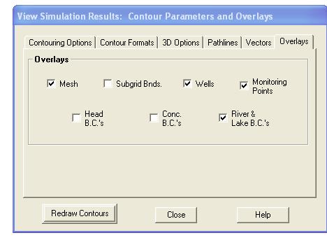
13 Output Time dialog. You may also use the + / - buttons to toggle through the output times. Under Plot and Contour Types you see that 2D (i.e., two-dimensional) plots are the default. Figure 12 A plan-view flood map through the middle of the aquifer is automatically generated (Figure 13). The AMR mesh is also shown as an overlay. The mesh overlay can be turned off by unchecking the Mesh box in the Contour Options dialog (under the Overlays tab; Figure 14). Figure 15 is the same x-y slice through the plume without the grid overlay. 13

14 Figure 13 Figure 14 14

15 Figure 15 You can change the slice coordinate by selecting the Go To button or the Layer no. +/- buttons (Figure 12). Further, you can view an animation of the different plan-view slices by changing the Animation Type to Layer (K-plane) and clicking the Start Animation button. Note: the layer number refers to the Adaptive Mesh Refinement (AMR) mesh associated with the multi-level AMR grid created during the simulation. In highly-refined mesh areas the vertical discretization is equal to the grid spacing in the highest-level subgrid (e.g, Level 5 in this example which utilizes five AMR levels). In less-refined areas the grid layer thickness for the output is equal to the grid spacing in the most-refined subgrid (e.g., Level 1, 2, 3, or 4). For any of these illustrations, you can save the plot format (and import it later) by clicking on the Save Plot Format button at the bottom of the View Simulation Results dialog. You can also print or export drawings in various graphics formats using the File > Print/Export option in the main menu. 15

16 Step 2 Plot Groundwater Pathline If groundwater pathline starting locations are defined in the input data (Pathlines > Assign in the main menu) their computed trajectories can be shown in the output by checking the Show Pathlines box in the Contour Options dialog (under the Pathlines tab; Figure 16). Check the with Time Markers box to add specified travel-time symbols. If the Include Retardation box is checked the pathline length and travel-time markers are based on the pore velocity divided by the retardation factor. Figure 16 Step 3 Cross-Section View of Plume To display the cross-sectional view of the plume in Figure 17, click on the X-Z Slice (Row) button in the lower left hand corner (red circle), and then select a row of cells going through the center of the plume (or select View > Change View Plane in the main menu). When you first switch to the cross-section view, you will want to add vertical exaggeration (e.g., VE = 10-20) by going to View > Vertical Exaggeration in the main menu. 16

17 Figure 17 Figures 18 (no grid overlay; see travel-time marker specification in red box) and 19 (with AMR mesh overlay) are vertical (x-z) cross-section views of the plume, including a groundwater pathline with 5-year travel time markers. 17

18 Figure 18 18

19 Figure 19 Figure 20 is a close-up view of the plume and the pore velocity vectors (activate under the Vectors tab in the Contour Options dialog). You can change the vector length [ V Length(%) ] and spacing ( Vector Indices Skip ) under the Vectors tab. 19

20 Figure 20 As usual, you can Zoom In, Zoom Last, or Translate the view by clicking one of the icons in the upper-left corner of the display (Figure 17) or by making the appropriate selection under View in the main menu. Step 4 3D Volume Plot of Plume Create a three-dimensional volume plot of the plume by selecting the 3D Volume radio button in the View Simulation Results dialog. Click on the Contour Options button to load the Contour Parameters and Overlays dialog (Figure 21). Click on the Contour Options tab and change the concentration contour range to mg/l. 20

21 Figure 21 Select the 3D Option tab in the Contour Parameters and Overlays dialog (Figure 21). Activate the first blanking parameter (click checkbox) and select C (mg/l) as the blanking parameter. Select the.le. operator and enter a value of mg/l to blank all cells with C.LE mg/l. Click the Redraw Contours button to view an isosurface of the central core of the plume. Now add a second blanking parameter to also view a slice through the plume. Click the + button and activate Y (m) (y-coordinate) as a blanking variable and enter y.le. 880 m. Click the - button to return to the first blanking variable (C) and select.or. as the logical operator. Click the Redraw Contours button to view a drawing similar to Figure

22 Figure 22 Note: the two blanking variables and logical operator are now: C.LE mg/l.or. y.le. 880 m Zoom in by increasing the Magnification to 1.5 and reduce the vertical exaggeration by increasing the Aspect Ratio to 2.0. Translate the drawing to the left by changing the x Translation to -10. Click Redraw Contours. Finally, show the computed groundwater pathline (activate under the Pathlines tab). You may also generate a higher resolution plot by changing to the High Graphics Resolution under the Contour Options tab (click Redraw Contours to generate). 22

23 Step 5 3D Fence Diagram of Plume Under Plot and Contour Types, choose the 3D Fence Diagram radio button (Figure 23). Click the Set Fence Type button, and in the Fence Diagram Type child dialog change (scroll) the fence diagram type to I- & K-planes. Click OK in the Fence Diagram Type child dialog. NOTE: you can increase the plot resolution to high resolution for final hardcopy output by selecting the Contour Options button, but the screen redraw times are longer. Figure 23 Step 6 Define Fence Diagram Type and Slice Locations Click on the Set Fence Location button, and choose the following locations (Figure 24; you can also vary the values as you wish): y-z planes: x =1617 m, x = 2001 m, x = 2348 m, x = 2610 m, and x = 2995 m (hold down the ctrl key to select multiple planes); x-y plane: z = 26.4 m. When you are finished, click the OK button and the plot is automatically regenerated (C blanking is added in the next step). 23

24 Figure 24 Step 7 Add Concentration Blanking to Fence Diagram Concentration blanking is also used to generate the fence diagram. Click on the Contour Options button and make the following changes in the 3D Options tab (Figure 25). The C blanking option renders any model areas with concentrations less than mg/l transparent. Click the Redraw Contours button to refresh the screen. Figure 26 is the final plot. Figure 25 24

25 In Figure 26 you could also blank parts of the plot based different combinations of x-, y-, and z- coordinates. For example, you could activate x.ge. 1,000 m as the second blanking variable and use.or. as the logical operator. In this case, any portion of the 3D model domain in which either C.LE mg/l or x.ge. 1,000 m would be blanked. Conversely, selecting.and. as the logical operator would only blank regions where both C.LE mg/l and x.ge. 1,000 m. Similarly, you could blank portions of the model domain in the y- and/or z-directions by adding third or fourth blanking variables. Figure 26 The 3D Graphics Viewing options include: view angle [ Rotation (around z-axis) and Elevation (tilt about horizontal axes)]; translations of the plot in any of the three coordinate directions; changes in the overall plot size ( Magnification ; increasing the magnification is similar to zooming in); and the plot aspect ratio (increasing the Aspect Ratio reduces the 25

26 vertical size of the plot; decreasing the Aspect Ratio is analogous to vertical exaggeration in cross-section diagrams). Selecting the Fit to Full Size button restores the default view parameter values and fits the simulation domain to the axes. 26