DCSP-10: Applications

Size: px

Start display at page:

Download "DCSP-10: Applications"

Dominic Goodman
6 years ago
Views:

1 DCSP-10: Applications Jianfeng Feng Department of Computer Science Warwick Univ., UK

2 Applications Power spectrum estimate Image Sampling theorem

3 Applications Power spectrum estimate Compression Image Sampling theorem

4 Understanding the plot Sampling rate is F s, the largest (fastest) frequency from the data is then F s /2 Remembering that our frequency domain is in [0 2p] which matches to [0 F s ] Divide [0 F s ] into N intervals and plot abs X[k] against kf s /N which gives power against frequency Since it is symmetric, we sometime only plot out [0, F s/ /2] Here F s =1 0 Hz

5 Spectrogram In real life example, all signals change with time (music for example) Using sliding window to sample signals and calculate PSD -- STFT

6 ; A Matlab Example close all clear all load handel; figure(1) plot(y); xlabel('time') T=size(y); for i=1:t(1,1) fre_x(i)=i*fs/t(1,1); end figure(2) plot(fre_x, abs(fft(y))) xlabel('hz') figure(3) spectrogram(y,128,120,[],fs); T1=floor(T(1,1)/2); omega1=1000; for i=1:t(1,1)-t1; z(i,1)=y(i,1)+.3*cos(2*pi*omega1*i/fs); end omega2=2000; for i=t-t1+1:t(1,1); z(i,1)=y(i,1)+.3*cos(2*pi*omega2*i/fs); end figure(5) plot(z); xlabel('time') figure(6) plot(fre_x,abs(fft(z))) xlabel('hz') figure(7) spectrogram(z,128,120,[],fs); for i=1:t(1,1); zn(i,1)=y(i,1)+.3*randn(1,1); end figure(8) plot(zn); xlabel('time') figure(9) plot(fre_x,abs(fft(zn))) xlabel('hz') figure(10) spectrogram(zn,128,120,[],fs); Three signals

7 ; A Matlab Example Original signal close all clear all load handel; figure(1) plot(y); xlabel('time') T=size(y); for i=1:t(1,1) fre_x(i)=i*fs/t(1,1); end figure(2) plot(fre_x, abs(fft(y))) xlabel('hz') figure(3) spectrogram(y,128,120,[],fs); T1=floor(T(1,1)/2); omega1=1000; for i=1:t(1,1)-t1; z(i,1)=y(i,1)+.3*cos(2*pi*omega1*i/fs); end omega2=2000; for i=t-t1+1:t(1,1); z(i,1)=y(i,1)+.3*cos(2*pi*omega2*i/fs); end figure(5) plot(z); xlabel('time') figure(6) plot(fre_x,abs(fft(z))) xlabel('hz') figure(7) spectrogram(z,128,120,[],fs); for i=1:t(1,1); zn(i,1)=y(i,1)+.3*randn(1,1); end figure(8) plot(zn); xlabel('time') figure(9) plot(fre_x,abs(fft(zn))) xlabel('hz') figure(10) spectrogram(zn,128,120,[],fs); + disturbance + noise

8 ; A Matlab Example close all clear all load handel; figure(1) plot(y); xlabel('time') T=size(y); for i=1:t(1,1) fre_x(i)=i*fs/t(1,1); end figure(2) plot(fre_x, abs(fft(y))) xlabel('hz') figure(3) spectrogram(y,128,120,[],fs); T1=floor(T(1,1)/2); omega1=1000; for i=1:t(1,1)-t1; z(i,1)=y(i,1)+.3*cos(2*pi*omega1*i/fs); end omega2=2000; for i=t-t1+1:t(1,1); z(i,1)=y(i,1)+.3*cos(2*pi*omega2*i/fs); end figure(5) plot(z); xlabel('time') figure(6) plot(fre_x,abs(fft(z))) xlabel('hz') figure(7) spectrogram(z,128,120,[],fs); for i=1:t(1,1); zn(i,1)=y(i,1)+.3*randn(1,1); end figure(8) plot(zn); xlabel('time') figure(9) plot(fre_x,abs(fft(zn))) xlabel('hz') figure(10) spectrogram(zn,128,120,[],fs); Abs(fft) vs Frequency

3*cos(2*pi*omega1*i/fs); end omega2=2000; for i=t-t1+1:t(1,1); z(i,1)=y(i,1)+.

9 ; A Matlab Example close all clear all load handel; figure(1) plot(y); xlabel('time') T=size(y); for i=1:t(1,1) fre_x(i)=i*fs/t(1,1); end figure(2) plot(fre_x, abs(fft(y))) xlabel('hz') figure(3) spectrogram(y,128,120,[],fs); T1=floor(T(1,1)/2); omega1=1000; for i=1:t(1,1)-t1; z(i,1)=y(i,1)+.3*cos(2*pi*omega1*i/fs); end omega2=2000; for i=t-t1+1:t(1,1); z(i,1)=y(i,1)+.3*cos(2*pi*omega2*i/fs); end figure(5) plot(z); xlabel('time') figure(6) plot(fre_x,abs(fft(z))) xlabel('hz') figure(7) spectrogram(z,128,120,[],fs); for i=1:t(1,1); zn(i,1)=y(i,1)+.3*randn(1,1); end figure(8) plot(zn); xlabel('time') figure(9) plot(fre_x,abs(fft(zn))) xlabel('hz') figure(10) spectrogram(zn,128,120,[],fs);

10 ; A Matlab Example close all clear all load handel; figure(1) plot(y); xlabel('time') T=size(y); for i=1:t(1,1) fre_x(i)=i*fs/t(1,1); end figure(2) plot(fre_x, abs(fft(y))) xlabel('hz') figure(3) spectrogram(y,128,120,[],fs); T1=floor(T(1,1)/2); omega1=1000; for i=1:t(1,1)-t1; z(i,1)=y(i,1)+.3*cos(2*pi*omega1*i/fs); end omega2=2000; for i=t-t1+1:t(1,1); z(i,1)=y(i,1)+.3*cos(2*pi*omega2*i/fs); end figure(5) plot(z); xlabel('time') figure(6) plot(fre_x,abs(fft(z))) xlabel('hz') figure(7) spectrogram(z,128,120,[],fs); for i=1:t(1,1); zn(i,1)=y(i,1)+.3*randn(1,1); end figure(8) plot(zn); xlabel('time') figure(9) plot(fre_x,abs(fft(zn))) xlabel('hz') figure(10) spectrogram(zn,128,120,[],fs);

11 A Matlab Example Will come back to it in the next few weeks after we learn how to design filters

12 Image Processing two-dimensional signal x[n 1,n 2 ], n 1,n 2 Z indices locate a point on a grid pixel grid is usually regularly spaced values x[n 1,n 2 ] refer to the pixel s appearance

13 Image Processing Gray scale images: scalar pixel values color images: multidimensional pixel values in a color space (RGB for example) we can consider the single components separately:

14 DFT for image DFT for x N 2-1 N X[k 1,k 2 ] = å 1-1 å x[n 1, n 2 ]exp(- 2p jk 1 n 1 ) exp(- 2p jk 2 n 2 ) n 2 =0 n 1 =0 N 1 N 2 IDFT for X x[n 1, n 2 ] = 1 N 2-1 N å 1-1 å X[k 1, k 2 ]exp( 2p jk 1 n 1 ) exp( 2p jk 2 n 2 ) N 1 N 2 k2 =0 k 1 =0 N 1 N 2

15 Example I clear all close all figure(1) I = imread('peppers.png'); imshow(i); K=rgb2gray(I); figure(2) F = fft2(k); figure; imagesc(100*log(1+abs(fftshift(f)))); colormap(gray); title('magnitude spectrum'); figure; imagesc(angle(f)); colormap(gray) Original picture Gray scale picture

16 Example I

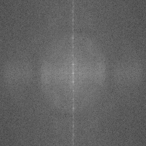
17 Example I FF=(100*log(1+abs(fftshift(F)))); for i=1:384 for j=1:512 ss=sqrt((i-192)*(i-192)+(j-256)*(j-256)); if(ss>100) FF(i,j)=0; end end end All low frequency information is here figure; imagesc(ff); colormap(gray); title('magnitude spectrum'); figure; imagesc(angle(ff)); colormap(gray)

18 Example I FF=(100*log(1+abs(fftshift(F)))); for i=1:384 for j=1:512 ss=sqrt((i-192)*(i-192)+(j-256)*(j-256)); if(ss>100) FF(i,j)=0; end end end All low frequency information is here figure; imagesc(ff); colormap(gray); title('magnitude spectrum'); figure; imagesc(angle(ff)); colormap(gray)

19 Example I? FF=(100*log(1+abs(fftshift(F)))); for i=1:384 for j=1:512 ss=sqrt((i-192)*(i-192)+(j-256)*(j-256)); if(ss>100) FF(i,j)=0; end end end All high frequency information is here figure; imagesc(ff); colormap(gray); title('magnitude spectrum'); figure; imagesc(angle(ff)); colormap(gray)

20 Example II Image processing

21 Example III: mind reading IDFT2

22 Sampling and reconstruction The question we consider here is under what conditions we can completely reconstruct the original signal x(t) from its discretely sampled signal x[n].

23 Sampling and reconstruction Theorem (Nyquist-Shannon sampling thm) Exact reconstruction of a continuous-time signal from its samples is possible if the signal is bandlimited and the sampling frequency is greater than twice the signal bandwidth Proof. The proof is again an application of FT, but we will not go through it here Please read around. It is based upon the sinc function.

24 Summary of FT At the end of the day, FT for signal x is only fft(x) it is deadly easy Hopefully and I am sure it will be useful for your future career

25 Summary of FT At the end of the day, FT for signal x is only fft(x) it is deadly easy Hopefully it will be useful for your future career I am proud of this

26 Filter A filter is a device or process that removes from a signal some unwanted component or feature. Filtering is a class of signal processing, the defining feature of filters being the complete or partial suppression of some aspect of the signal. Most often, this means removing some frequencies and not others in order to suppress interfering signals and reduce background noise.

27 Filter

28 A Filter will look like this Received signal x [n] (lifted it up for 5 units for visualization)

29 A Filter will look like this y ([i] = ( x[i] + +x [i-n]) / (N+1) N=9 here

30 A Filter will look like this y ([i] = ( x[i] + +x [i-n]) / (N+1) N=9 here

31 A Filter will look like this y ([i] = ( x[i] + +x [i-n]) / ( N+1) N=9 here

32 A Filter will look like this y ([i] = ( x[i] + +x [i-n]) / (N+1) N=9 here This filter is called moving average MA(10)

33 A Filter will look like this You might be able to guess what is the original signal

34 A Filter will look like this y ([i] = ( x[i] + +x [i-n]) / (N+1) + (y[i-1]+ y[i-n])/n This filter is called auto-regressive moving average ARMA(p,q)

35 A Filter will look like this y ([i] = ( x[i] + +x [i-n]) / (N+1) + (y[i-1]+ y[i-n])/n This filter is called auto-regressive moving average ARMA(p,q)

36 N th order filter Filter In general, we can include both the input x [n-k] and the previous outputs y [n-k] to generate y(n) = a 0 x(n)+a 1 x(n-1)+ +a N x(n-n) +b 1 y(n-1)+ +b N y(n-n)

37 Example In this case, when b i =0, it is an MA y(n) = [ x(n)+ x(n-n) ] / N In general it is called ARMA filter. AR for auto-regressive

38 DCSP-11: Filter Jianfeng Feng Department of Computer Science Warwick Univ., UK

39 Aim To find the coefficient a s and b s for certain purposes: for example, filter out noise, stop certain band signals, allow certain band signal to pass etc.

40 A Trick {y(n)} = a 0 {x(n)}+a 1 {x(n-1)}+ +a N {x(n-n)} +b 1 {y(n-1)}+ +b N {y(n-n)} Multiplying z -n on both size of the equation above where z is a complex number and summing over n Y(z) = a 0 X(z)+a 1 z -1 X(z)+ +a N z -N X(z) +b 1 z -1 Y(z)+ +b N z -N Y(z) Y(z)-( b 1 z -1 Y(z) + + b N z -N Y(z)) = a 0 X(z) + a 1 z -1 X(z) + + a N z -N X(z)

41 A Trick [1-b 1 z b N z -N ] Y(z) = [ a 0 + a 1 z a N z -N ] X(z) Y(z) ={ [ a 0 +a 1 z a N z -N ] / [1-b 1 z b N z -N ] } X(z) = H(z) X(z) H(z) is usually called transfer function: it characterizes the input output relationship of a filter

42 A Trick Y(z) ={ [ a 0 +a 1 z a N z -N ] / [1-b 1 z b N z -N ] } X(z) = H(z) X(z) For example, when z = exp(j w ) Y( w ) = H (w) X (w) X and Y are actually the DTFT of x and y In particular, look at a specific frequency w 0, for example Y( w 0 ) = H (w 0 ) X (w 0 ) The magic of FT!!!!!

43 A Trick Y( w 0 ) = H (w 0 ) X (w 0 ) H (w 0 ) = 1 the signal will not be affected at all H (w 0 ) = 0, the signal is stopped your ideas for developing filter?

44 Nonrecursive Filters When a filter is nonrecursive, its difference equation can be written y(n) = a 0 x(n) + a 1 x(n-1) + + a N x(n-n) Such filters are also called finite impulse response filters, for the obvious reason that their IR contain only finitely many nonzero terms. Correspondingly, the TF of a nonrecursive filter can be written as N å m=0 H(z) = a m z -m

45 Block diagram

46 Block diagram a N a N-1 z a 1 a 0

47 Three types of representation Linear difference equation Block diagram Transfer function

48 Zeros Trying to figure out how an MA filter will behave, is not always so simple. Another way of looking at it is through its frequency domain behaviors. We can make a start on this by examining the zeros of its transfer function H(z), i.e. those values of z for which H(z)=0 since H(z) is a polynomial of order N with real coefficients,

49 Zeros Trying to figure out how an FIR filter will behave, is note always so simple. Another way of looking at it is through its frequency domain behaviors. We can make a start on this by examining the zeros of its transfer function H(z), i.e. those values of z for which H(z)=0 H(z) is a polynomial of order N with real coefficients, the complex conjugate root theorem states that if P is a polynomial in one variable with real coefficients, and a + bi is a root of P with a and b real numbers, then its complex conjugate a bi is also a root of P

50 Zeros We can express H(z) in terms of the roots by writing N N z H( z) ( z z ) m 1 where in general z m = z m exp ( j arg [z m ] ) is the mth root, or zero of the transfer function. m The zeros of a transfer function are usually denoted graphically in the complex z-plane by circles, as shown in the following Fig.

51 Zeros

52 Recursive Filters Of the many filter transfer function which are not MA, the most commonly use in DSP are the recursive filters, so called because their current output depends not only on the last N+1 inputs but also on the last N outputs.

Digital Signal Processing Lecture Notes 22 November 2010

Digital Signal Processing Lecture otes 22 ovember 2 Topics: Discrete Cosine Transform FFT Linear and Circular Convolution Rate Conversion Includes review of Fourier transforms, properties of Fourier transforms,