A New CAD/CAM/CAE Integration Approach to Modelling Flutes of Solid End-mills

Transcription

1 A New CAD/CAM/CAE Integration Approach to Modelling Flutes of Solid End-mills Li Ming Wang A Thesis In the Department of Mechanical and Industrial Engineering Presented in Partial Fulfillment of the Requirements For the Degree of Doctor of Philosophy at Concordia University Montreal Quebec, Canada September 2014 Li Ming Wang, 2014

2 This is to certify that the thesis prepared CONCORDIA UNIVERSITY SCHOOL OF GRADUATE STUDIES By: Entitled: Li Ming Wang A New CAD/CAM/CAE Integration Approach to Modelling flutes of Solid End-Mills and submitted in partial fulfillment of the requirements for the degree of complies with the regulations of the University and meets the accepted standards with respect to originality and quality. Signed by the final examining committee: Doctor of Philosophy (Mechanical Engineering) Dr. Chun Wang Chair Dr. Deyi Xue External Examiner Dr. Leon Wang External to Program Dr. Mingyuan Chen Examiner Dr. Ramin Sedaghati Examiner Dr. Zezhong (Chevy) Chen Thesis Supervisor Approved by Chair of Department or Graduate Program Director Dean of Faculty

3 ABSTRACT A New CAD/CAM/CAE Integration Approach to Modelling Flutes of Solid End-mills Li Ming Wang, PhD. Candidate Concordia University, 2014 Milling is used widely as an efficient machining process in a variety of industrial applications, such as the complex surface machining and removing large amounts of material. Flutes make up the main part of the solid end-mill, which can significantly affect the tool s life and machining quality in milling processes. The traditional method for end-mill flutes design is using try-errors based on cutting experiments with various flute parameters which is time- and resources-consuming. Hence, modeling the flutes of end-mill and simulating the cutting processes are crucial to improve the efficiency of end-mill design. Generally, in industry, the flutes are ground by CNC grinding machines via setting the position and orientation of grinding wheel to guarantee the designed flute parameters including rake angle, relief angle, flute angle and core radius. However, in previous researches, the designed flute profile was ground via building a specific grinding wheel with a free-form profile in in the grinding processes. And the free-form grinding wheel will greatly increase the manufacturing cost, which is too complicated to implement in practice. In this research, the flute-grinding processes were developed with standard grinding wheel via 2-axis or 5-axis CNC grinding operations. For the 2-axis CNC flute-grinding processes, the flute was modelled via calculating the contact line between the grinding wheel and cutters. The flute parameters in terms of the iii

4 dimension and configuration of grinding wheel were expressed explicitly, which can be used to planning the CNC programming. For the 5-axis CNC flute-grinding processes, the flute was obtained with a cylinder grinding wheel via setting the wheel s position and orientation rather than dressing the dimension of grinding wheel. In this processes, optimization method was used to determine the wheel s position and orientation and evaluating the machined flute parameters. Beside, based on the proposed flute model, various conditions for grinding wheel s setting were discussed to avoid interference of flute profile. A free-form flute profile is consequently generated in its grinding processes. However, in the end-mill design, the flute profile is simplified with some arcs and lines to approximate the CAD model of end-mills, which would introduce errors in the simulation of cutting processes. Based on the proposed flute-grinding methods, a solid flute CAD model was built and a CAD/CAM/CAE integration approach for the end-mill was carried out to predict the cutting forces and tool deflection. And also, the prediction results with various methods are verified to demonstrate the advantage of proposed approach. This work lays a foundation of integration of CAD/CAM/CAE for the end-mill design and would benefit the industry efficiently. iv

5 ACKNOWLEDGEMENTS My deepest gratitude goes first and foremost to Professor Chevy Zezhong Chen, my supervisor, for his constant encouragement and guidance. He has walked me through all the stages of PhD s research, which benefits me with valuable research experiences and skills. Without his consistent and illuminating instruction, this thesis could not have reached its present form. I also owe my sincere gratitude to my friends, especially for my colleagues in the Lab, who gave me their generous help and advice in my studying and daily life. I would like to mention the engineers from Cutting-tool Design Company that benefited me a great deal for their advice and suggestions. Last my thanks would go to my beloved family and fiancée for their loving considerations and great support for me over these four years.. v

6 Table of Contents List of Figures... ix List of Tables... xiii Chapeter 1. Introduction Basics of end-mills Mechanism of milling processes Flute of end-mills Literature review Geometric model of end milling cutter Cutting forces in milling processes Research Problems & Objectives Proposed objectives Overview of proposed technical route Dissertation Organization Chapeter 2. 2-axis CNC flute-grinding with standard grinding wheel Introduction Basics of the 2-axis CNC grinding of end-mill flutes Parametric representation of a standard grinding wheel The flute machining configuration Mathematical model of the machined flute Formulation of the rake and the flute angles CNC programming for wheel parameters determination Relationship between the flute rake angle and the wheel parameters Relationship between the flute angle and the wheel parameters Applications Summary Chapeter 3. Research on the moment of inertia of end-mill flutes with the CAD/CAM integration model Introduction vi

7 3.2 Representation of flute shape Two-arc model Free-form model Calculation of area and moment of inertia The discritised method Statistical formulation of the inertia with various flute shapes Model Verification Application Summary Chapeter 4. Wheel position and orientation determination for 5-axis CNC flute-grinding processes Introduction Flute profile modeling with 5-axis CNC grinding Grinding wheel modeling aixs flute-grinding processes Flute parameters formulation within the cross-section Investigation of wheel s position and orientation on flute profile Contact area for the grinding wheel and cutter Interference of flute profile Solution for the wheel s position and orientation Modeling the optimization problem Verification Summary Chapeter 5. Application of CAD/CAM/CAE integration to predict cutting forces and tool deflection of end-mills Introduction CAD/CAM Integration for modeling end-mill Flute modeling Flank surface modeling Validation of the proposed CAD model Cutting Forces prediction vii

8 5.4 Tool deflection prediction Distribution of cutting forces Cantilever beam model for tool deflection Validation and application Summary Chapeter 6. Conclusions and future work References viii

9 List of Figures Figure 1.1 Illustration of solid end-mills Figure 1.2 Application of end mill in the milling processes Figure 1.3 Flute model of end mills Figure 1.4. Illustration of grinding end-mills... 6 Figure 1.5 Illustration of standard grinding wheels and dimensions Figure 1.6 Cross-section of 4-flute end mills: (a) Kivanc s model (b) Improved model Figure 1.7 Geometry and kinematics of the flute grinding operation.[16] Figure 1.8. Boolean operation in flute-grinding processes [19] Figure 1.9. Modeling the grinding processes of solid end-mills Figure 2.1 Illustration of the dimensions of the standard grinding wheel selected in this work and the wheel coordinate system Figure 2.2 Illustration of the wheel position in terms of the tool bar in the 2-axis flute grinding.30 Figure 2.3 Simulation of the 2-axis flute grinding with a standard wheel Figure 2.4 Illustration of the contact curve between the grinding wheel and the flute Figure 2.5 The segments of the flute profile on the cross section Figure 2.6 Plots of rake angles in terms of the wheel set-up angle and its dimensions Figure 2.7 Plots of the flute angles in terms of the wheel set-up angle and its dimensions Figure 2.8 The plot of the flute angles of the flute in terms of the wheel dimensions, H 1 and Figure 2.9 The solid flute models (a) to (e) by using the wheel dressed with the solution 1 to 5, respectively ix

10 Figure 3.1. The deflection model of solid end-mill: (a) cylindrical beam model (b) real model. 55 Figure 3.2. Illustration of 2-flute and 4-flute shapes Figure 3.3. Two-arc models for 2-flute and 4-flute end-mill Figure 3.4 Calculation of area and moment of inertia Figure flute shapes with different tool radius and core radius Figure 3.6. Variation of inertia regarding to tool radius with different core ratio for 4-flute shapes Figure 3.7. Variation of scaling factor in 4-flute power equations with the core ratios Figure 3.8. Various 2-flute shapes with different tool radius and core radius Figure 3.9. Variation of inertia about X axis regarding to tool radius with different core ratios for 2-flute shapes Figure Variation of scaling factors in 2-flute power equations with the core ratios Figure 3.11 Variation of inertia about Y axis regarding to tool radius with different core ratios for 2-flute shapes Figure 3.12 Variation of scaling factors in 2-flute power equations with the core ratios Figure Deflection of end-mill with various geometrical parameters: (a) Core ratio, (b) Tool radius and (c) suspended length Figure 4.1 Illustration of the cylindrical grinding wheel Figure axis CNC flute-grinding processes Figure 4.3 Flute profile generated by envelope of grinding wheel Figure 4.4 Projection of cutter profile and wheel edge within cross-section Figure 4.5 Simulation for the interference in the flute-grinding processes Figure 4.6 Flute shapes with various position and orientation x

11 Figure 4.7 Interference for flute profile within cross-section Figure 4.8 Flute grinding with various condition : (a) non-interference, (b) critical condition and (c) interference condition Figure 4.9 Illustration of flute-grinding model Figure 4.10 Flowchart of calculation of 5-aixis flute-grinding model Figure 4.11 Initial points for the optimization Figure 4.12 Solution for the wheel positon and orientation Figure 4.13 Flute proflie and parameters with the solution : (21.585, ,43.437) Figure 4.14 Equality constraints in the input processes Figure 4.15 Plot of the objective function: (a) 3D surface (b) Contour Figure 4.16 The solid flute model simulated by CATIA Figure 5.1 CAD/CAM integration for end-mill Figure 5.2 Illustration of the cutting-edge-grinding process Figure 5.3 Solid CAD model of the end-mill generated by CATIA Figure 5.4 End-mill manufactured with CNC grinding machine Figure 5.5 Moment of inertia I y along the tool axis Figure 5.6 Meshing of the cutter-workpiece Figure 5.7 Cutting simulation with ThirdWave Figure 5.8 Cutting forces prediction with the developed CAD model Figure 5.9 Comparison of proposed model and approximation model Figure 5.10 Cutting forces prediction with the approximation model Figure 5.11 Illustration of cutting forces measurement Figure 5.12 Cutting forces measured by experiment xi

12 Figure 5.13 Cutting forces prediction with different methods Figure 5.14 Cutting forces in the milling processes Figure 5.15 Cutting forces prediction flowchart Figure 5.16 Cutting forces measured for AISI Figure 5.17 Predicted milling forces for AISI Figure 5.18 Elemental cutting forces (Fy-max) distributed along the tool axis Figure 5.19 Unit loading algorithm for predicting the tool deflection Figure 5.20 Tool deflection prediction with FEA Figure 5.21 Tool deflection prediction with different models Figure 5.22 Tool deflection with various cutting depth xii

13 List of Tables Table 2.1 The values of the flute and the wheel parameters of the examples Table 2.2 Five selected solutions of H 1 and to the flute angle (80 degrees) Table 2.3 The measured rake and flute angles of flute models in simulation and their errors Table 3.1 Comparison of measured and predicted flute inertia Table 3.2. Deflection of end-mills with various geometrical features Table 4.1 Parameters for flute-grinding process Table 4.2 Verification of optimized model Table 5.1 Tool parameters of the developed CAD model and manufactured cutter Table 5.2 Material properties of the end-mill and work-piece Table 5.3 Machining parameters Table 5.4 Maximum cutting forces with proposed model Table 5.5 Maximum cutting forces with the approximation model Table 5.6 Machining condition for experiment Table 5.7 Maximum cutting forces with experiments Table 5.8 Machining parameters and average cutting forces with ThirdWave Table 5.9 Cutting coefficients of AISI xiii

14 Chapeter 1. Introduction Milling is used widely as an efficient machining process in a variety of industrial applications wherever the complex surface machining, removing large amounts of material. According to the International Institution of Production Research (CIRP), cutting tools nearly make up 30% of all the manufacturing cost [1, 2]. Due to its flexible operation, large material removing rate and high surface quality, cutting tool is one of the most important economic considerations in metal cutting process [3]. However, because of the complex structures of milling cutters, it is difficult to develop its accurate geometric model. 1.1 Basics of end-mills Total length Shank length Flute length Helix angle Cutter Diameter Gash Land Radial primary relief angle Radial secondary relief angle Short tooth Flute Primary land Secondary land Axial secondary relief angle Axial primary relief angle Long tooth Figure 1.1 Illustration of solid end-mills. 1

15 The milling cutter is generally manufactured using the CNC grinding machine through the specific commercial CAM software in industry. A typical end milling cutter is shown in Figure 1.1. It consists of four basic features: shank, flute, tooth and gash. Shank is the primitive shape of end-mill with a rotation features, such as cylindrical, cone, and it can be mounted on the tool holder with some specific and standard connection. Generally, the basic shape of shank was made by power metallurgy and then ground with CNC machine to guarantee the design tolerance and surface quality. Flute is the most important feature of the milling cutters. It formed the most important tool parameters in the flute structures including rake angle, relief angle, core radius, flute angle and helix angle, which will be elaborated in the following introduction and research. Tooth and gash are located at the bottom of milling cutter, which form the bottom cutting edge and enable the face milling at the bottom. According to the number of flutes or teeth, the end-mills are classified as 2, 3, 4-tooth cutters commonly. Generally, the more tooth, the high feed rated can be applied in the machining processes and also the better surface quality would be obtained. It is obvious that flutes make up the main part of the body. And the space of the flute will greatly affect the chip evacuation and dynamic performance. It is helpful to design flute shape to get suitable cutting performance [4-7]. Besides, with the advance of CNC technology, the precision of cutter is increasing, and it also brings kinds of features such as, the gashes, variable pitch and etc. In this thesis, we focus on modeling of the flute shape and flute parameters via modeling its manufacturing processes with different methods. 2

16 1.11 Mechanism of milling processes The performance of milling process is determined by the mechanism between the cutting tools held in a high-speed rotating spindle and the work-piece. A four-tooth down milling operation is shown in Figure 1.2.The milling cutter is in process with a varying and periodic chip thickness, which produces various cutting forces. Based on different cutting condition, one or more teeth are in cut with the work-piece [1, 8]. Therefore, the milling operation is an intermittent cutting process, which will result in the varying cutting forces. Feed Tool Holder Cutting Speed End-mill Workpiece Table Figure 1.2 Application of end mill in the milling processes. 3

17 Two basic problems in metal cutting are the cutting process efficiency and output quality such as the tool deflection, surface roughness. In order to balance the two aspects, continual researches have been done for centuries. A significant improvement in process efficiency may be obtained by optimizing the process parameters [9] including the cutting speed, feed-rate, cutting depth. Another method is to optimize the tool geometry, such as rake angle, relief angle, tool tip radius and so on. In this research, we will emphasis on the tool geometry, in other words, we will try to evaluate the cutting performance integrating the tool geometry with FEA method. However, for end milling cutter, aforementioned, it has a complex geometric structure. In the literature review, most of the researchers applied the simplified geometric models which use the lines and arcs to approximate the basic cutting angles. And the approximation differences between the simplified models and the real cutter model would introduce errors to the predictive results in the milling process. Besides, some researcher also pointed out that the predictive results depend on the accuracy of geometrical models [10]. Therefore, modeling the accurate geometrical features of end milling cutter is perquisite for the predicting cutting performance during milling process Flute of end-mills As mentioned, the flue is the main part in the milling cutter body. The geometric model is shown in Figure 1.3. It forms the important parameters such as rake angel, core diameter r c, flute (pitch) angle, and helix angle. In practice, the flute is machined by the grinding wheel moving with a helix motion, which will be discussed in the literature review section. 4

18 r T r c φ γ λ Figure 1.3 Flute model of end mills. The profile of flute plays important roles in the chip evacuation during the milling process. Generally, larger flute space is useful for the chip flowing, however, that will decrease the tool stiffness. Especial for the high strength material which will reach high temperature and larger cutting forces in the cutting process, this problem would be much more serious [11]. Therefore, in practice, the tool core radius is usually limited to no less than 0.6 times of the tool radius based on the engineering experience. In the literatures, especial in the tool deflection calculation, the flute is generally estimated as a cylinder with an equivalent radius as 0.8 times of tool radius [8]. With the CNC technology developing, a lot of new flute shapes appear, and this estimation is not suitable for all the shapes. Therefore, it is necessary to develop an accurate flute model to predict the dynamic behavior and improve tool design. Five or four axis CNC grinding machine is employed to program the grinding processes of end-mills and the NC programming is generated automatically through the specific commercial CAM software in industry. Figure 1.4 shows a general setting of grinding end-mills. The grinding wheel is mounted above the tool bar with a specific position and orientation relative to the grinding wheel in the machine coordinate system. With the intersection between 5

19 the grinding wheel and the tool bar, the flute shape of end-mill is formed based on the kinematics of the moving grinding wheel and cutter at each operation. It is difficult to model the exact three dimensional shapes of end mills, because a certain part of the shape is not determined until the actual machining operation [9]. Therefore, the accurate geometrical model of end-mill can only be developed via simulating and modeling its grinding processes. Besides, the flute parameters are also required to be guaranteed in the flute-grinding processes with a specific dimension and setting for the grinding wheel. Grinding Wheel Tool bar Base Figure 1.4. Illustration of grinding end-mills 6

20 As mentioned, the flute shape is closely related with the profile of grinding wheel applied in the grinding process. The grinding wheel is composed of a layer of abrasive diamond particle bonded together to formed its profile. Before using, the profile of grinding wheel should be measured and ground to guarantee its dimension. This operation is called dressing the grinding wheel. To reduce the cost of manufacturing end-mill, standard grinding wheel is always applied in industry. There are several types of standard grinding wheel with a basic geometrical profile: cylinder, cone and combination of both shown in Figure 1.5. In this research, standard grinding wheels are applied to modeling the flute-grinding processes. H Abrasive D Abrasive D H H2 Abrasive D H1 Figure 1.5 Illustration of standard grinding wheels and dimensions. 1.2 Literature review In this section, the related literature on the geometric model of end milling cutter, manufacturing process of flute, cutting forces prediction with milling processes are comprehensively reviewed. Besides, the comparison between linear cutting force model and 7

21 exponential cutting force model is presented. Through the reviews, we found the gaps in current methods and propose the objectives of this research Geometric model of end milling cutter As we mentioned, the structure of solid end-mill is very complex, for simplification, some early researches using cylinder model [12] to estimate the end milling cutter. This model is easy calculation for prediction of dynamic performance based on cantilever beam theory. Because of the effect of flute, an equality cylinder beam is recommended as 0.8 times [8] of the tool radius. However, such assumption ignored the flute shape of end-mill, such as the variation of core radius and the length of flutes. Therefore, the method is not accurate enough for calculating the deflection especially for slender tools. In order to raising the accuracy, another model is to assume the tool as a step beam with two sections. One section is for the shank and another for the flute. And the flute section is approximated with a two-arc profile shown in Figure 1.6 (a). Basically, the accuracy of this two section model is related with the difference of the approximated model and real flutes. Besides, taking 2-flute cutter for example, the area moment inertia of cross-section is not symmetrical in different directions; therefore, it cannot be modeled as a cylinder with uniform area moment inertia. From the above discussion, the only solution is to represent the real shape of the flute. Arcs [10, 13] are used as the approximation of the flute. As shown in Figure 1.6(a), the crosssection of 4-flute end mill is defined as two simple arcs ( ). The profile is governed by two key parameters: the flute depth fd and the BC s radius r. Kivanc [10] represent this model 8

22 using an equivalent radius R eq in terms of the radius r and the arc position. This model cannot reveal all the information of end mill, especially missing the key parameters: rake angle and relief angle. Besides, based on this structural model, Kivanc derived the area moment inertia to predict the static and dynamic properties of tools with different geometry and material via finite element analysis. A two section general equation for two-step cantilever beam deflection is formulated. And also the mode shape and natural frequencies of end-mills were predicted using the Euler-Bernoulli equations. However, the profile of the tool is far different to the real end mill in industry, and it ignored the most important flute parameters such as rake angle, relief angle, which will introduce errors to the predictive results. C F E α r D C rc B fd A rc γ B A γ fd : flute depth r : arc BC s radius r c core radius (a) γ : rake angle α : relief angle r c : core radius (b) Figure 1.6 Cross-section of 4-flute end mills: (a) Kivanc s model (b) Improved model. An improved model is proposed in Tsai s [14] research shown in Figure 1.6 (b). The profile comprise of five connected segments: three lines and two arcs for each flute. The basic parameters, such as tool radius rake angle, relief angle, the corresponding relief width FE 9

23 and EF (flank surface), rake width AB and core radius r c are also illustrated in the figure. The parametric representation of flute was derived a piecewise equations with five segments. Nevertheless, for the real end mill, the rake length is not a straight line, and the flute profile is free-form curve which is manufactured using grinding wheel. Therefore, the flute curve can be obtained through the kinematic relation of flute-grinding process. There are some papers focusing on the grinding methods of end mill, mainly building the flute shape [7,14-20]. Kaldor [15] first discussed two basic geometric problems in the flutegrinding processes: 1) The Direct Problem: the determination of the resulting flute profile for a given grinding wheel cross-section; 2) The Inverse Problem: the determination of the wheel profile for a desired flute crosssection. And also, in this research, the grinding wheel and cutter were defined with a mathematical representation. The result flute profile is obtained via CAD approach (image processes) which is to calculate the extreme point on the flute to form the contour of the flute with iteration processes. A programing package was developed in the research first to verify the direct problem and cited most in the following research. However, the accuracy of the flute model greatly depends on the iteration number. Due to the limitation of computer technology, the indirect problem was not discussed in the paper. 10

24 Figure 1.7 Geometry and kinematics of the flute grinding operation.[16] Following the above research, Ehmann [16] developed a program and presented a well solution for the indirect problem based on the principles of differential geometry. The kinematics of flute-grinding processes was elaborated via three frameworks: tool frame, machine frame, and the work-piece frame. The fundamental relationship between grinding wheel and cutter was established through the contact theory, that is the common normal at the contact point between the wheel surface and flute surface must intersect the axis the tool. Besides, he also pointed out that there is one unique relationship between the desired geometry of the flute cross-section and grinding wheel profile for a fixed machine setup and machine condition. This major contribution for this work was that the principle foundation for the contact points was deduced and solved. Kang [17, 18] gave a series papers on the detail calculation of the grinding processes base on the kinematics of grinding processes via CAD approach. A generalized mathematical model 11

25 for the inverse and direct problem for disk and axial-type tools was investigated in Kang s research. And the analytical solution for the resulting flute profile was provided. For the second part of this research [18], numerical solutions were developed with a calculation program and also the sensitivity analysis of the result flute profile in terms of the machining setting and grinding wheel profile errors were first investigated to identify the most sensitive parameters. Figure 1.8. Boolean operation in flute-grinding processes [19]. Recently, Kim [19] develop a more sophisticated CAD method (direct method) to obtain the machined shape of an end milling cutter using Boolean operations between a given grinding wheel and a cylindrical work-piece. The flute shape is obtained shown in Figure 1.8: a successive intersection between the work piece and wheel is iterated to get the final solid model, which is exactly the same with real cutter. The developed model can be used to verify the manufacture of rake angle and inner radius before the real grinding program implemented. 12

26 Furthermore, the solid CAD model can be accepted by most common software that would be used to FEA simulation to evaluate the cutting performance. In the following work, Kim and Ko [20] proposed a manufacturing model of flutegrinding processes (direct method), and gave the mathematical expression of the flue crosssection curve based on the envelope theory. The basic idea is discretize the grinding wheel as finite thin disk. Each disk would intersect with the cross-section after sweeping a volume. The swept disk is modeled using coordinate transformation. The program was integrated with the CAD/CAM system to generate the NC code, which was used to grind the end-mill for machining hardened steel. Chen [21] presented a method to grind rake face of taper end mill using a novel spherical grinding wheel for ball-end mill. In this work, the normal rake angle and helix cutting edge are ground uniformly via adjust the position and orientation of grinding wheel. And also, the cutting edge transition from the ball end to cone neck was guaranteed. Rather than previous research dedicated to the flute profile, the paper focused on the desired flute parameters-rake angle, which will greatly affect the cutting performance in the milling processes. Ren [22] developed a CAD/CAM integration method to grinding the flutes of end-mills with 2-axis CNC grinding machine. Nevertheless, most of those researches focus on shaping the helix flutes without considering modeling tool parameters including rake angle, core radius, flute angle and cutting edges (relief angle), which will affect the cutting performance most. It is difficult to model the exact three dimensional shape of an end mill because a certain part of the shape is not determined until the actual machining stage [20]. 13

27 Besides, in engineering, the flute-grinding processes cannot be simplified as the indirect or direct problem. Actually, in the CNC grinding processes, the grinding wheel is generally standardized, which means the shape of grinding wheel is constrained with some parameters. And the wheel position and location are required to be determined to guarantee the designed flute parameters. Until now, to the author s knowledge, there has been little work about modeling the flute parameters including rake angle, core radius, flute angle and cutting edges, and to determine the wheel s position and orientation. In order to solve the above problem, In this thesis, a parametric CAD model is provided base on the grinding processes including the helix flute, flank surfaces using the design parameters and grinding parameters based on modeling the kinematic of the grinding processes, that is CAD/CAM integration for end-mill Cutting forces in milling processes Cutting forces play an important role in the machining processes, such as the deformation of cutting tools, surface finish, tool wear, etc. Therefore, for decades, lots of research has been done on the mechanism of cutting processes so as to predict and optimize the cutting forces. In this work, cutting forces generated in milling processes will be considered as the criterion to evaluate the cutting performance of end-mills. The progress in formulating model of the milling processes must be based on the understanding of the mechanics of milling. Several models have been developed to derive cutting force, which can be classified into three types: 1) the experimental model, 2) the analytical model and 3) FEA model. 14

28 The early predictive models relied on empirical data to establish the forces. Obviously, this method will need much more experiments for different materials, cutters, and operating conditions. Sometimes, it cannot lead to a general predictive model for most of the conditions. However, because of its easy operation, it is still used widely in the field of engineering. Generally, for the experimental model, the cutting forces are considered as function of cutting processes parameters [23, 24], in terms of feed rate, cutting depth and cutting width shown in Eq. (1.1). x y z F Ca a f (1.1) p e Where, C is the cutting coefficients, and x, y, z is the exponential index, which should be determined experimentally; a p is the cutting depth and f is the feed rate. As mentioned in the introduction, the performance of milling process is determined by the mechanism between the cutting tools held in a high-speed rotating spindle and the workpiece. The cutting forces in the milling process can be predicted based on the analytical cutting force model [8, 25-30]. The milling forces is resolved into two direction: the tangential cutting force f t and the radial cutting force f r, which are respectively corresponding to the tangential and radial cutting forces in orthogonal cutting model. The major problem for analytical milling process is how to calculate the uncut chip thickness. In this research, a piecewise sinusoidal function is usually applied to estimate the chip thickness [8]: entry exit f sin, h 0, others, (5.2) 15

29 where, f is the feedrate per teeth; ф is the immersion angle shown in Fig. 2 and entry, exit are the entry and exit angle. There are two basic methods to calculate the cutting force with analytical model along the helix cutting edges: Numerical method and Integrate method [1,2,8,25-30]. A) Numerical method The milling cutter is divided into finite slides along the tool rotation axis. Using the linear cutting force model, the cutting force for each slide is represented in the matrix form: f khk dz, (5.3) N t tc te f r j1 krch k re where, dz is the discrete size in the rotation axis direction; N is the tooth number. In order to apply the cutting forces to predict the machining result, such as deflection, surface roughness, etc., normally, the cutting forces are resolved into X, Y direction via a transformation matrix: f N x cos sinkh tc kte dz f y j1 sin cos krch k. (5.4) re The total cutting force would be obtained by summing all the M element forces in Eq.(5.5). F M x fx F f. (5.5) y i1 y 16

30 B) Integrate method The integrate method is trying to get an analytical expression of the cutting forces through integrating the triangle function regarding to the immersion angle at different conditions. a F p N kh k x cos sin tc te dz F y z=0 j1 sin cos krch k, (5.6) re where, a p is the axial cutting depth. One important step for this method is to determine the effective boundary for the integration. It is summarized by Y. Altintas and E. Budak [1, 8] into six different cases based on the immersion angle with the rotation of end-mill. There are still other scientists using ANN [31-34] (Xu et al., 1994, Radhakrishnan 2005, Cus, et al., 2006, Zheng, 2008,) to estimate and control the forces in milling processes. The ANN approach requires neither rigorous knowledge of cutting mechanics nor the long development time. It is easy to get the result without considering the milling process based on complicated mathematical modeling approach. And in some cases, the results are acceptable as the theoretical approach. In this processes, the cutting forces considering the milling processes as a black box using neural network. In the black box system, the cutting parameters, tool parameters and workpiece properties as the input, while the outputs are cutting forces. Besides, the surface quality can also be discussed with the similar processes. The advantage of the neural network algorithm is greatly reducing the time-consuming of calculation work for the analytical method. But it also needs a training of the network with some experimental data. 17

31 In order to give some accurate and general model, some researchers simulated the milling processes via Finite element analysis (FEA) and the conventional cutting theory was used to predict the forces. A lot of researches [35-39] applied 2D simulation metal cutting with orthogonal cutting to predict cutting forces and temperature, but that does not exist physically. And all the milling processes are 3D cutting processes with oblique cutting in practice. Wu [40] used 3D FEA model to simulate the complex milling processes of titanium alloy (Ti6Al4V) with considering the dynamic effects, thermo-mechanical coupling, and material damage law and contact criterion with the software ABAQUS. The cutting forces, temperature, chip formation can be predicted. It was noted that the simulation processes can be fed back to improve the milling processes. Maurel-Pantel [41] developed an analytical finite element technique for simulation of shoulder milling operation on SISI 304L with end-mills. The approach was based on Lagrangian formulation using a penalty contact method. The prediction cutting forces by FEA was compared with experimental cutting force to show the validation of FEA. In the conclusion, the research pointed out that accurate tool geometry can be reconstructed and used in the simulation processes to improve the predictive results. But lot difficulties appear to exist in defining a complex CAD model, which will be a major topic in our research. Tool deflection caused by cutting forces in the milling processes will greatly affect the surface quality, especially for some slender tool or low-rigidity part. FEA is an efficient technology to predict the tool deflection. Ratchev and Liu, [42, 43] presented a virtual environment using 3D finite element technology for low-rigidly part system, which was able to compute cutting forces and the result surface error due to the tool deflection. It provided a 18

32 potential prospect of NC verification that considering of dynamic behavior of the cutters and part, which can be used in the optimization of tool path planning. Besides, the FEA results for cutting processes can also be used to improve the cutting performance of cutters. Abele [44] first presented a representation of twist drill geometry including all the design parameters which related to the drilling processes. A GA method was used to optimize the geometry of drill. The most novel and historic contribution is that the torsional stiffness, torsional stability, drilling torque, coolant flow and chip evacuation are quantized with mathematical expression and integrated with a fitness function. The FEA method was implemented in the research to calculate the drill stiffness and stability. And also the flute grindabiltiy was used as a constraint to check the validation of optimization results. Similarly, a 3D representation of flat end-mill include flutes in terms of surface patches and shank was proposed by Tandon [45] with CAD algorithm. The modelled end-mill was used to study the cutting flutes under static and transient dynamic load conditions. This research offered an efficient way for the design of flat end-mill in the concept stage. However, the geometry used in above FEA simulation is simplified, which has a great effect on the accuracy of the predication. And, the analysis process is also very time-consuming. Therefore, the software which can provide accurate information for end mill geometry and performed calculation and simulation of milling processes is in a great need nowadays. 1.3 Research Problems & Objectives According to reviewing the prior literatures, the geometry and mechanical model of endmill has been studied by many researchers. Those studies provided us a general direction in theory and technology: 19

33 1. The accurate geometric model of end-mill can be obtained from modeling its manufacturing (grinding) processes, which is the CAD/CAM integration technology; 2. Flutes as the major part of end-mill is determined by the shape of grinding wheel and the orientation and position in the grinding operation. The mathematical models of flute faces and curves of end-mill can be calculated via vectors and analytic geometry. 3. Modeling and FEA simulation of the milling processes is critical and efficient for the cutting force estimation. And accurate geometric model of end-mill in the machining are required. However, for current researches, there are three problems to be solved in this research: With the CNC technology advances, the grinding process of end-mill becomes easy to operate and more versatile. The profile of flute is determined by the shape grinding wheel and operation in grinding process (position and orientation). Although, the direct and inverse methods for has been developed by some pioneers researches, the flute is made by standard grinding wheel, which imply that the shape of the grinding wheel cannot be modified randomly. Therefore, to grind the designed flute with standard grinding wheel is a great challenge in this dissertation. As mentioned, the flute involves many key parameters such as rake angle, relief angle, core radius, which complicate the calculation of modeling the geometry. To the author knowledge, there are few literatures to formulate of the flute parameters generated from the grinding processes. 20

34 Some research used some arc and lines to represent in the geometry models of flutes in the CAD system which is different with the real cutter. Besides, the geometrical difference inevitably introduce errors in the prediction of cutting performance with FEA simulation, such as cutting forces and tool deflection. And, this model cannot combine the grinding process effectively Proposed objectives In order to solve the proposed problem, the following objectives are set to contribute in the end-mill research field. The first objective is to develop the kinematic model of the grinding processes of flutes and formulate the design parameters including rake angle, relief angles, core radius, and flute angle via differential geometry and coordinate transformation. Hereto, a solid CAD model of end-mills can be proposed with the CAD/CAM technology. The second objective is to determine position and orientation of standard grinding wheel for the designed flutes with CNC grinding operation. First, the designed flute is defined by the flute parameters in the first objective. And then an automatic CNC programing is required to determine the operation of grinding wheel via solving the representation of flute parameters in terms of wheel position and orientation. The third objective to implement CAD/CAM/CAE in the simulation of milling processes to improve the accuracy of cutting force and tool deflection prediction. 21

35 1.3.2 Overview of proposed technical route To achieve the above mentioned objectives, following technical route is proposed. The major work is to develop the 3D flute model of end-mill based on the kinematic grinding processes with integration of the CAD/CAM system. As mentioned, five axes CNC grinding machine is generally employed to construct the grinding processes of end mill and the NC programming is generated automatically through the grinding wheel operation planning. The shape of end mill is formed through intersection between cutting tool and grinding wheel. Thus proper wheel geometries must be determined prior to machining the helical flute for the end mills designed. The basic procedure shown in Figure 1.9 can be described as: inputting the design parameters and determining the grinding operation referring to the position and orientation, while, outputting the result shape through the calculation of operation of the grinding wheel. The key point in this step is to determine the wheel position and orientation. To solve this problem, first, the kinematic relation is required to build up for each operation. Then, based on the envelope theory to find out the contact curve or envelope profile generated by the grinding wheel, that is, for each point located on the wheel, the velocity is perpendicular to the normal of the wheel surface. As a result, the formulation for the designed parameters will be deduced from the result surface within the cross-section. In addition, the above method can also be reversed to adjust the grinding wheel dimension and operations. 22

36 Design parameters Grinding processes (CAM) CAD model of end- -mill 1. Rake angle 2. Core radius 3. Flute angle 4. Tool radius 5. Helix angle 6. Flute length 1. Wheel radius 2. Wheel angle 3. Wheel width Grinding Wheel Helix flutes 1. Land width 2. Relief angles 1. Position 2. Orientation Cutting edges Figure 1.9. Modeling the grinding processes of solid end-mills. In the literature review, the simulation-based milling processes are introduced briefly. In this research, the advantage of proposed CAD/CAM integration approach is combined with the FEA simulation to predict the cutting forces and tool deflection in milling processes. First the cutting coefficients are obtained through the cutting simulation for different cutting depth and feed rate with the developed CAD model of end-mill. The distribution of milling forces can be predicted with the cutting coefficients under machining condition. The tool can be regards as a cantilever beam with different cross-section while calculating the tool deflection. And the area moment inertia has been obtained from the developed CAD model. According to the unit-loading beam theory, the tool deflection is derived through summing the affect caused by distribution forces. 23

37 1.3.3 Dissertation Organization In this chapter, a basic introduction and comprehensive review were carried out on the end-mills modeling and its application. For the following sections, the basic structure of this dissertation is organized as follows. Chapter 2 developed a flute model with the 2-axis CNC grinding processes via calculating its contact line in the 3D space, which can be used to modeling the flute profile and program the CNC grinding processes. Chapter 3 discussed the effect of moment initial with various flute profile based on the CAD/CAM integration proposed in Chapter 2. However, for the 2-axis CNC grinding, there will be some limits such as, wheeldressing and interference-checking. Hence, Chapter 4 presented a 5-axis CNC grinding processes and also a novel method is proposed to determine the wheel position and orientation in the grinding processes. In Chapter 5, based on the proposed flute-grinding model, a CAD/CAM/CAE integration approach was implemented to evaluate the cutting forces and tool deflection in the milling processes. Finally, Chapter 7 contains the summary and future work of this work. 24

38 Chapeter 2. 2-axis CNC flute-grinding with standard grinding wheel 2.1 Introduction End-mills are widely used in CNC machining, and their helical flutes are crucial to their cutting performance. In industry, these flutes are usually defined with four parameters: the helical angle, the (radial) rake angle, the flute angle (pitch angle), and the core radius; and they are specified in the end-mill design. To grind the flutes, two-axis CNC tool grinding machines are often employed. During the 2-axis flute grinding, the wheel self-rotates in high speed and moves forward along the tool axis in a specified feed, while the tool bar rotating in a specified angular velocity. It is required that the flute parameters specification should be guaranteed after grinding. Since the wheel parameters the grinding wheel dimensions and the wheel set-up angle determine the machined flute parameters, the wheel parameters should be determined according to the flute specifications, which is conducted in the flute CNC programming prior to grinding. Unfortunately, the relationship between the wheel parameters and the flute parameters is very difficult; as a result, the wheel parameters are currently approximated on trial-and-error. This method is quite time-consuming and in-accurate. To improve quality of cylindrical endmills, it is in high demand that a new approach to determining the wheel parameters in CNC programming. Technically, it could be an effective solution to derive explicit formulae of the flute parameters with regard to the wheel. The main stream of the research on grinding flutes of end-mills and drills could be classified into two groups, the direct and the inverse (or indirect) methods which has been introduced in the Chapter 1. As mentioned, the direct method is to compute the flute shape 25

39 generated in the 2-axis or the 5-axis CNC grinding, based on the machining parameters of the given wheel And, the inverse method is to calculate the curved profile of a non-standard wheel based on the given flute of an irregular end-mill, which will be ground with this wheel in the 2- axis grinding. Ehmann and DeVrise [16] and Kang et al. [17, 18] proposed a direct method of modeling the flute shape generated with a given wheel in the 2-axis grinding. The principle of these methods is that, at any point of the 3-D contact curve between the wheel and the flute at a moment of grinding, the wheel velocity is perpendicular to the wheel surface normal. Hsieh [46] extended the above methods from the 2-axis to the 5-axis flute grinding. It should be noted that these direct methods are for the drill flutes. Different from the above methods, Pham and Ko [47] tried to find 2-D cross-sectional profiles of end-mill flutes ground on 2-axis machines. The mechanism of this method is to regard the wheel as a pile of thin disks, to find the profiles of the material on the cross-section cut by the disks, and to compute the envelope of the profiles, which is the flute profile. Unfortunately, Pham and Ko did not provide the equation of the flute profile for end-mill modeling. Besides the aforementioned direct methods, the existing indirect (inverse) methods are to find the profile of a wheel according to the profile of an end-mill flute and the wheel position in the 2-axis grinding. The principle of these methods is that, at any point of the contact curve between the wheel and the flute, the flute surface normal passes through the wheel axis. The research of the articles [48-53] applied the principle on different end-mills. In general, the calculated wheel profiles are complicate curves, and thus, the wheels are irregular and nonstandard. Moreover, some researchers [45, 54] have used the Boolean operations in CAD software to construct solid models of end-mills in order to predict their cutting performance in machining simulation. Unfortunately, all the above methods cannot be used in CNC 26

40 programming for the 2-axis grinding of the end-mill flutes with their parameters specified. Here, the CNC programming is to determine the dimensions of a standard wheel, its location and orientation to ensure the prescribed flute parameters. Although Kim et al. [19] proposed a CNC programming method, they used the Boolean operations to construct end-mill solid models, which is time-consuming, less accurate, and with large file size. Chen and Bin [21] rendered a 5- axis CNC programming method for grinding the rake face of a tapered end-mill. To establish an effective and accurate approach to CNC programming for the 2-axis grinding of cylindrical end-mill flutes, our work adopts a standard wheel and derives closed-form equations of the radial rake angle and the flute angle in terms of the wheel parameters, the wheel dimensions and the wheel set-up angle. By applying these equations, the wheel parameters can be efficiently and accurately determined in the CNC programming. In this work, first, the basics of the 2-axis CNC grinding of cylindrical end-mill flutes are introduced. Second, the mathematical model of the flute is established. Third, the closed-form equations of the rake angle and the flute angle are derived. Then, the relationships between the flute and the wheel parameters are discussed for CNC programming. Finally, several examples are rendered to demonstrate the validity and advantages of this new approach. 2.2 Basics of the 2-axis CNC grinding of end-mill flutes Parametric representation of a standard grinding wheel In industry, there are many types of standard grinding wheel available, and a popular wheel type is selected in this work. Figure 2.1 illustrates this type of standard grinding wheel and its 27

41 dimension notations. The wheel radius R and thickness H 2 refer to the wheel size, and the dimensions, H 1 and, refer to the wheel profile. Grinding wheels with different dimensions generate different rake and flute angles and different flute shapes in the 2-axis flute grinding. Thus, the wheel dimensions should be determined in the CNC programming. Referring to practice, the wheel radius and thickness are chosen according to the available wheel size, and the H 1 and are two parameters of the wheel in this work. Y g Y g R O g h Z g O g θ X g α H 1 H 2 Figure 2.1 Illustration of the dimensions of the standard grinding wheel selected in this work and the wheel coordinate system. To represent the wheel s revolving surface in a parametric form, a wheel coordinate system XYZO g g g g is established shown in Figure 2.1. The origin O g is at the center of the larger end of the wheel, and the Z g axis is along the wheel axis from the larger end to the smaller end. The X g and Y g axes are on the larger end and perpendicular with each other. In the wheel coordinate system, the parametric representation of the wheel h 28 W can be derived as g,

42 where h 0, H 2, 0, 2, and h h R cot cos W g h, R cot sin, (2.1) h h 0,0 h H1 h H,H h H (2.2) The equation of the normal vector of the wheel surface is derived as following, cos N g h, sin, (2.3) h where h 0,0 h H1 cot,h h H 1 2. (2.4) The flute machining configuration Currently, a lot of tool manufacturers produce cylindrical end-mills on 2-axis CNC tool grinding machines. To machine the end-mill helical flutes, the grinding wheel is set up so that it is right above the tool bar with the distance between the wheel and the tool axes (denoted as d) and these axes form angle. This angle is called the wheel set-up angle in this work, and it is fixed during machining. Figure 2.2 illustrates the machining configuration of the 2-axis flute grinding. In this machining, the wheel rotates swiftly and moves along the tool axis in a 29

43 specified feed v. Simultaneously, the tool bar rotates in a specified speed. In this configuration, distance d is equal to the core radius r C plus the wheel radius R. The wheel setup angle determines the rake angle of the machined tool, hence, it is a wheel parameter. To ensure the prescribed rake angle, this angle is not equal to the flute helical angle and should be accurately calculated in the CNC programming. Y g Z g X g β O g Y t d X t Z t O t Figure 2.2 Illustration of the wheel position in terms of the tool bar in the 2-axis flute grinding. 2.3 Mathematical model of the machined flute To determine the above-mentioned wheel parameters for a flute design, the wheel dimensions, H 1 and, and its set-up angle,, the conventional way is to grind end-mill flutes 30

44 by trial and error. However, it is costly and time-consuming. Now, an effective solution is to establish the mathematical model of the machined helical flute by using the parametric representation of the grinding wheel and the kinematics of the flute machining configuration. Based on this configuration, from a geometrical point of view, the wheel sweeps an imaginary volume during machining, and the external surface of this volume is in the same shape as the machined flute surface. Theoretically, the external surface can be modeled using the envelope theory. At any moment of the machining, the external surface of the volume contacts the flute at a curve, which is called the contact curve at this moment. According to the envelope theory, the wheel surface normal at any point of the contact curve is perpendicular to the corresponding wheel velocity with respect to the tool bar. Therefore, the flute geometry consists of all of the contact curves during machining. To establish the mathematical model of the contact curve, the grinding wheel should be represented in the tool coordinate system, which is established in the following. Figure 2.3 Simulation of the 2-axis flute grinding with a standard wheel. 31

45 To establish the tool coordinate system XYZO, T T T T the origin O T is at the center of the tool bottom, the Z T axis is along the tool axis and pointing to the tool shank, and the axes are perpendicular to each other and on the tool bottom plane (see Figure 2.2). The X T and Y T X T axis is horizontal and the Y T axis is vertical. According to the aforementioned wheel set-up in the 2- axis flute grinding, the parametric representation of the grinding wheel in the tool coordinate system can be found. First, the wheel coordinate system is assumed to coincide with the tool coordinate system. Second, the grinding wheel is translated along the Y T axis by the distance d. Then, the grinding wheel is rotated around the Y T axis by the wheel set-up angle. Therefore, the equivalent transformation matrix is cos 0 sin R r sin 0 cos C M 1. (2.5) In the 2-axis flute grinding, the grinding wheel moves along the tool axis in feed rate v, and, at the same time, the tool bar is rotated in angular velocity, (clockwise in terms of the Z T axis. The kinematics of this grinding is equivalent to that the tool bar is stationary and the wheel moves along a helix of the same helical angle as with the feed rate v along the tool axis and the angular velocity in counter-clockwise. The equivalent kinematics is useful to find the instantaneous velocity at any point on the wheel during machining. Due to the helical angle, the relationship between the feed rate v and the angular velocity is 32

46 v cot. (2.6) r T is T r cot system is From a geometric point of view, the value of can be simply set as 1, so the feed rate v. The corresponding matrix of the kinematics represented in the tool coordinate t t t t cos sin 0 0 sin cos 0 0 M 2 t (2.7) rt cot t where t represents the machining time. Therefore, the grinding wheel can be represented at any machining time t in the tool coordinate system as W T h,, t R r Rhcotcos coscos t R hcotsinsin t hsin cos t RrC sin t R h cot cos cos sin t R hcot sin cos t h sin sin t C cos t.(2.8) rt cot thcos Rhcotsin cos According to the above equation, the instantaneous velocity of the wheel in the tool coordinate system can be calculated as V T R h cot cos cos sin t R hcot sin cos t h sin sin t RrC cos t R h t h t RrC t. h,, t R h cot cos cos cos t cot sin sin sin cos sin rt cot (2.9) To formulate the machined flute in this work, it is necessary to find the envelope of the wheel in machining with the envelop theory. At any moment of machining, the grinding wheel contacts the flutes at a curve, which is on the envelope surface. The main feature of this contact 33

47 curve is that, at any point of the contact curve, the wheel surface normal is perpendicular to the instantaneous velocity. Here, the wheel surface normal in the tool coordinate system is denoted as N T, and the equation of the contact curve is N V. (2.10) T T 0 For a helical flute of cylindrical end-mills, the contact curves at different machining time are the same in shape. Therefore, the flute surface can be generated by sweeping the contact curve at the beginning t 0 along the helical side cutting edge. Assume the points of the contact curve are represented as h,, t, which is h,,0 here. It is not difficult to find the equation of this contact curve as T cot sin cos cos sin 0 sin h cos cos R h cot sin r cot sin cos cos h. (2.11) RrC R h h By solving this equation, the relationship between h and of the contact curve points can be found as follows. 0h H, If 1 T C h r cot Rr cot cot ; (2.12) H h H, and, if 1 2 h * c 1 2 1cot sin rt ct o cos cotcot Rr cot cot cos RH cot cotsin. (2.13) 34

48 Now, the contact curve can be partially found in the tool coordinate system by substituting Eq. (2.12), Eq. (2.13), and t 0 into Eq. (2.8). Specifically, the two segments C 2 C 3 and C 4 C 5 of this contact curve on the two revolving surfaces of the wheel can be found (see Figure 2.4). In addition, the coordinate xt,, y 5 T,, z C C5 T, C 5 of the point C 5 satisfies an equation 2 2 x C y C r. Thus, the parameters of the points C 2, C 3, C 4, and C 5, which are T, 5 T, 5 T h,,0 C2 C, 2 h,,0 C3 C, 3 h,,0 C4 C 4, and h,,0 C5 C 5, respectively, are known. Since these surfaces are not continuous in terms of their first derivatives, the segments C 2 C 3 and C 4 C 5 are disconnected. Moreover, in the helical fluting, the wheel circular edges, E 1 and E 2, grind part of the flute. In some cases, the wheel circular edge E 3 could generate the flute shape, which is not discussed here. Unfortunately, the envelope theory cannot be applied on finding the contact curve in the flute grinding with the edges. It is evident that an arc on each of the edges, E 1 and E 2, are contact curve segments. In Figure 2.4, the arc C 3 C 4 of the edge E 2 is a contact curve segment connecting C 2 C 3 and C 4 C 5 ; and the arc C 1 C 2 of the edge E 1 is a contact curve segment. The representations of C 1 C 2 and C 3 C 4 can be found easily. 35

49 C 5 C 1 C 3 C2 C 4 Z T Y T O T X T Figure 2.4 Illustration of the contact curve between the grinding wheel and the flute. According to Eq. (2.8) of the wheel representation in the tool coordinate system, the equation of the contact curve segment C 1 C 2 on the edge E 1 is derived with t as zero and h as zero, which is R cos cos C 12 RrCRsin, and, C1 C 2. (2.14) R sin cos where the parameter C of the point C 1 1 is * C R r r C T R rc cot 2 arcsin cot, and Rsin R sin. (2.15) R r r C T RrC cot 2 arcsin cot, and Rsin R sin 36

50 Similarly, the equation of the contact curve segment C 3 C 4 on the edge E 2 can be found by setting t as zero and h as H 1, which is C H1 sin Rcoscos Rr Rsin, and, C3 C 4. (2.16) H1 cos R sin cos 3-4 c After finding all the points h,,0 of the contact curve, the flute surface F t is generated by sweeping the contact curve along the helical movement of the wheel. So the equation of the flute surface is R h cotcos cos cos t R h cotsin sin t h sin cos t RrC sin t. (2.17) R h cot cos cos sin t R h cot sin cos t h sin sin t C cos t h cos R h cotsin cos rt cott F t R r 2.4 Formulation of the rake and the flute angles As convention, the rake and the flute angles of a cylindrical end-mill flute are defined on the flute profile within the cross-section. Since the flute profiles on different cross-sections are the same in shape, the cross-section of z T as zero is taken in this work. To find the flute profile P on this cross section, first, the following equation is obtained. T h cos R h cot sin cos r cott 0. (2.18) Then, by solving this equation, the machining time t is calculated as t h, R h cot sin cos h cos. (2.19) r cot T 37

51 Finally, the flute profile equation is found by substituting Eq. (2.19) into Eq. (2.17). It is easy to understand that this profile consists of several segments, which are co-related to the contact curve segments on the revolving surfaces and the circular edges of the wheel. Figure 2.5 shows four segments of the flute profile, P 1 P 2, P 2 P 3, P 3 P 4, and P 4 P 5, which are co-related to the four contact curve segments, C 1 C 2, C 2 C 3, C 3 C 4, and C 4 C 5, respectively. The parameters of the points, P 1, P 2, P 3, P 4, and P 5, are h,, t C2 C2 P, 2 h,, t C3 C3 P, 3 h,, t C4 C4 P 4, and h,, t C5 C5 P, 5 respectively. P 1 P 4 P 3 P 2 γ P 5 Ф O T Figure 2.5 The segments of the flute profile on the cross section. To formulate the rake angle of the side cutting edge, the equation of the flute profile segment P 1 P 2 should be derived. Since the points of the flute profile P 1 P 2 are on the edge E 1, 38

52 their parameter h is zero. According to Eq. (2.19), the equation of the machining time for the flute profile segment P 1 P 2 is Rsin cos tp. (2.20) 12 r cot T And the equation of the profile segment P 1 P 2 is P 1-2 P 1-2 P 1-2 C P 1-2 P 1-2 P1-2 C P 1-2 Rcos t cos cos Rsin t sin Rr sin t Rsin t cos cos Rcos t sin Rr cos t where, C1 C 2. Thus, the machining time 1 t P of the point P 1 is tp C 12 1, (2.21), and the position vector of the point P 1 is P C. Then, according to Eq. (2.21), the tangent vector T P C of P 1 P 2 at the point P 1 is where * 1 * * 2 C1 Rrc1R1sin C R 1 2cos cos C 1 1cot r * T cot sin T P R sin sin 12 C 1 C 1 * 1 * * 1cot C 1 Rrc2 R2sin C R 1 1cos cos C 1 2cot rt cot sin R sin cos 1 cos rt cot C1 Therefore, the rake angle can be calculated as cot R sin cos C, and 2 sin rt cot C P C , (2.22). (2.23) arccos P1 2 T. (2.24) To formulate the flute angle of the flutes, the position vector of the point P 5 on the cross section of zt 0 should be found. According to Eq. (2.19), the machining time t P of this point 5 39

53 is thc, C. By substituting the parameter 5 5 h,, t C5 C5 P5 of the point P 5 into Eq. (2.17), its position vector of P 5 is the x T and T flute angle is y coordinates of F hc, C, t P Hence, the formula of the * arccos P1 2 C P. (2.25) CNC programming for wheel parameters determination The main objective of CNC programming is to determine the wheel parameters to ensure the pre-specified values of the flute parameters after machining. Basically, the CNC programming is an iterative process of modifying the wheel dimensions and its position (its location and its set-up angle) and evaluating the machined flute parameter values. In this work, the wheel of standard shape with the dimensions, R, H 1, H 2, and shown in Figure 2.1, is employed in the 2-axis grinding of the cylindrical end-mill flutes. It is practical that the wheel is made by dressing an existing wheel, of which the R and H 2 are often kept the same and the H 1 and are changed to the values that are calculated by using the flute angle equation derived in above section. The location of the wheel can be easily determined according to the configuration of the 2- axis flute grinding. To ensure the core radius, the distance between the wheel and the tool axes is R r C ; therefore, the origin of the wheel coordinate system is an offset of the origin of the tool coordinate system along the Y T axis by r C. The wheel set-up angle is determined according to the rake angle equation derived in Section 2.4. The closed-form equations of the rake and the 40

54 flute angles are crucial to determining the wheel parameters more efficiently and accurately, compared to the prior direct methods. For better CNC programming, the relationships of the wheel parameters and the flute parameters are discussed in the following Relationship between the flute rake angle and the wheel parameters According to the equation of the rake angle, it is related to the wheel set-up angle, the wheel radius R, the tool radius r T, the core radius r C, and the helical angle. Usually, the grinding wheel radius R and thickness H2 are often determined according to an existing grinding wheel available in the company. Thus, for a flute with the r T, r C, and specified, the wheel set-up angle can be determined for the specified. It is worth to mention that the wheel parameters H 1 and do not affect the rake angle. Four examples are provided to demonstrate the relationship between the rake angle and the wheel parameters. For these examples, the flute parameters, the helical angle, the tool radius r T, and the core radius r C, are 35 degrees, 10 mm, and 6 mm, respectively. In the first example, the wheel dimensions are provided in Table 2.1, and the wheel set-up angle varies between 10 to 80 degrees. By Eq. (2.24), the rake angles are calculated with different wheel set-up angle, and the plot of the rake angles is shown in Figure 2.6. It is evident that the rake angle varies dramatically, changing from -28 to 58 degrees. In the second example, the wheel radius R increases from 20 to 150 mm, and the other wheel parameters are listed in Table 2.1. On the contrary, the rake angle decreases from 15.5 to 9.5 degrees. The plot of the rake angle is shown in Figure 2.6(a) and Figure 2.6(b). In the third and the forth examples, the 41

55 wheel dimensions, H 1 and are changed, respectively. But, the rake angle remains unchanged, and the plots are displayed in Figure 2.6(c) and Figure 2.6(d). Table 2.1 The values of the flute and the wheel parameters of the examples. Example 1 Example 2 Example 3 Example 4 Wheel radius R (mm) Wheel dimension H (mm) 2 H Wheel dimension 1 (mm) Wheel angle (Degree) Wheel set-up angle (Degree)

56 Rake angle ϒ (⁰ ) (a) Wheel-setup-angel β (⁰) Rake angle ϒ (⁰ ) (b) Wheel-radius R (mm) 43

57 Rake angle ϒ (⁰ ) (c) Wheel-height H 1 (mm) Rake angle ϒ (⁰ ) (d) Wheel-angle α (⁰) Figure 2.6 Plots of rake angles in terms of the wheel set-up angle and its dimensions. 44

58 2.5.2 Relationship between the flute angle and the wheel parameters For the flute angle of the flute, it is mainly related with the wheel parameters, R, H 1,, and. To demonstrate the relationship between the flute angle and the wheel parameters, the flute angles are calculated in the aforesaid examples 1 to 4, and the corresponding flute angle curves are plotted in Figure 2.7. It can be observed that the flute angle decreases while increases in Example 1, and the flute angle increases while R, H 1, and increase in Example 2, 3, and 4, respectively Flute angle φ (⁰ ) (a) Wheel-angle α (⁰) 45

59 Flute angle φ (⁰ ) (b) Wheel-radius R (mm ) Flute angle φ (⁰ ) (c) Wheel width H 1 (mm) 46

60 Pitch angle φ (⁰ ) (d) Wheel-Set up angle (⁰) Figure 2.7 Plots of the flute angles in terms of the wheel set-up angle and its dimensions. In CNC programming, first, R and H 2 are determined based on an available grinding wheel. Second, according to the prescribed rake angle, the wheel set-up angle can be determined. Then, by Eq. (2.25), the flute angles can be calculated in terms of different values of H 1 and. For the prescribed flute angle, a group of solutions of H 1 and can be found. Among these solutions, one pair of H 1 and can be determined according to the available grinding wheel. To illustrate this practical approach, an example is rendered here. In this example, the tool radius r T is 10 mm, the core radius r C is 6 mm, the rake angle is 10 degrees, and the helical angle is 35 degrees. Suppose a wheel with R as 50 mm and H 2 as 47

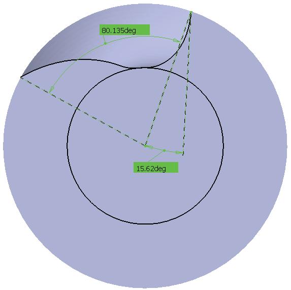
61 20 mm is available and it is to be dressed for grinding the flute. According to the rake angle, the wheel set-up angle should be 45 degrees. Then, by changing H 1 between 0 to 10 mm and between 25 to 90 degrees, the flute angles can be computed, and the flute angle surface is plotted in Figure 2.8. Since the flute angle should be 80 degrees, the red curve on the flute angle surface represents the options of H 1 and. According to the shape of the available wheel, one pair of H 1 and on the red dash curve that is close to the actual wheel size is chosen to dress the wheel into the required wheel in order to grind the flute. Solutions to flute angle of 80 H1 Figure 2.8 The plot of the flute angles of the flute in terms of the wheel dimensions, H 1 and. 48

62 2.6 Applications To demonstrate validity of this new CNC programming approach to determining the dimensions and position of a standard wheel for the 2-axis flute grinding of a cylindrical endmill, a practical example is provided and the results are discussed. In this example, the flute is designed with its parameters specified and is to be machined on a 2-axis CNC grinding machine. The tool radius r T is 10 mm, the core radius r C is 5.5 mm, the flute helical angle is 35 degrees, the rake angle is 15.5 degrees, and the flute angle is 80 degrees. This example shows the details of the CNC programming of wheel parameters determination. Suppose a grinding wheel of radius R as 50 mm and thickness H 2 as 20 mm is available in the machine shop. Here, it is employed to machine the flute. Thus, its dimensions, H 1 and, and its location and set-up angle should be determined in the CNC programming. Then, the wheel is dressed according to the values of H 1 and. Before the 2-axis flute grinding, the wheel is set up according to its location and the set-up angle in terms of the tool bar. In this approach, the wheel is offset along the Y T axis so that the distance between the wheel and the tool axes is R r C. To ensure the prescribed rake angle (15.6 degrees), the wheel set-up angle can be calculated as 45 degrees. To ensure the flute angle (80 degrees), many pairs of H 1 and are the solutions, five of which are selected and listed in Table

63 Table 2.2 Five selected solutions of H 1 and to the flute angle (80 degrees). Wheel parameters Solution1 1 Solution2 2 Solution3 3 Solution4 4 Solution5 5 Wheel dimension H 1 (mm) Wheel angle (degree) In practice, suppose the available grinding wheel can be dressed with one of the solutions. After dressing, the wheel can be used to grind the flute on a 2-axis CNC grinding machine. In this work, the flute grinding process is simulated in CATIA, and the solid models of the flutes generated with the wheel of different H 1 and are attained, which are shown in Figure 2.9. The rake and the flute angles of the solid flute models are measured in CATIA. The results are listed in Table 2.3, and it is clear that the errors of the rake and the flute angles are very small. Besides, the acceptable tolerance for the flute parameters in engineering is around 1 degree for angle and 0.1 mm for length. The main reason of these errors, we believe, is the error of constructing the solid flute models. Therefore, the CNC programming to wheel parameters determination is accurate. 50

64 (a) (b) 51

65 (c) (d) 52

66 (e) Figure 2.9 The solid flute models (a) to (e) by using the wheel dressed with the solution 1 to 5, respectively. Table 2.3 The measured rake and flute angles of flute models in simulation and their errors. Flute parameters Solution Solution Solution Solution Solution Specified rake angle (degree) Measured rake angle (degree) Rake angle error 0.3% 0.1% 0.1% 0.6% 1.2% Specified flute angle (degree)

67 Measured flute angle (degree) flute angle error 0.03% 0.1% 0.1% 0.04% 0.3% 2.7 Summary This work has proposed a new approach for automated and accurate CNC programming to determine the dimensions and orientation of a standard wheel in the 2-axis flute grinding of cylindrical end-mills. The main contribution of this work is the formulation of the rake and the flute angles in terms of the wheel parameters and the practical method of determining the wheel dimensions according to a wheel available in machine shops. Using this approach, the CNC programming is automated and accurate, instead of trial and error. Examples have demonstrated the validity of this approach, which can be implemented in tool manufacturers. This approach provided and integration approach for CAD/CAM of cylindrical end-mill. 54

68 Chapeter 3. Research on the moment of inertia of end-mill flutes with the CAD/CAM integration model 3.1 Introduction The performance of the milling process is determined by the mechanism between the end-mill held in a high-speed rotating spindle and work-pieces [3,8,25]. Consequently, tool deflection and vibration are caused in this process. Generally, End-mill is regarded as the most flexible part in the machine structure, which makes the largest contribution to the tool deflection and dynamic behavior. In industry, the core radius is usually limited to no less than 0.5 times of the tool radius to guarantee proper rigidity. Hereto, the tool stiffness would greatly determine machining accuracy and surface quality. A A-A Cylindrical beam 0.8 r T (a) A B B-B Shank Flute r c r T (b) B L 2 L 1 Figure 3.1. The deflection model of solid end-mill: (a) cylindrical beam model (b) real model. 55

69 In most studies [10,55-59], the solid end-mill is generally assumed as a cantilever cylindrical beam rigidly supported by the tool holder. Base on the cantilever beam model, Kline [55] predicted the surface error caused by the static deflection in the milling processes. To improve the accuracy of deflection prediction, Kops [56] proposed that the equivalent diameter of the cylindrical beam is approximately 80% of the cutter diameters shown in Figure 3.1(a). In Elbestawi s research [57], the tool stiffness was calculated using the cantilever beam bending theory and a dynamic milling model was presented. Recently, Xu [58] developed a more sophisticated dynamic milling model with considering the cutter flexibility to predict not only the tool deflection but also the dynamic surface errors. Clearly, all of these models is based on the cantilever beam with a cycle cross-section (Figure 3.1 (a) A-A), which ignores the variety of flute shapes. Hence, it inevitably introduces errors in the following deflection or surface error prediction. Solid area Flute space Core radius Core radius Figure 3.2. Illustration of 2-flute and 4-flute shapes. In practice, as shown in Figure 3.1(b), the solid end-mill consists of two geometrical parts: the shank and the flutes. As one major part of end-mills, flutes have significant effect on the tool stiffness. With advances of manufacturing of end-mill, the flute shapes are designed with a variety of structures, such as 2-flute and 4-flute shapes illustrated in Figure 3.2. Therefore, the 56

70 flute shapes should be considered in the evaluation of tool stiffness, especially for the variety of core radius. A detail investigation about the flute shape models will be elaborated in the following section. According to the beam bending theory, the tool stiffness can be evaluated through the moment of inertia. In order to investigate the effect of flute shapes, the inertias of flute crosssection are discussed in this work. For simplification, the inertia of the moment is simplified as inertia in the following description. In this chapter, an efficient and exact solution of calculating the inertia of solid end-mill flute was introduced, which can contribute to the accuracy of prediction of tool deflection and dynamic behavior. The outline of this work is organized as follows. Section 2 discusses two different geometrical flute shape models. Section 3 presents a finite method of calculating the inertia of flute cross-section. Besides, through fitting the inertia data for various flute shapes, an efficient power model in term of tool radius and core radius is proposed to predict the inertia. The proposed approach is compared with current model to show the accuracy. Finally, an application is undertaken. 3.2 Representation of flute shape Since flutes are critical for the tool geometry, developing of the mathematical representation of flute shape is the first step of calculating the moment of inertia. Throughout the literature reviews [7,10,17,19,60], according to the representation of flute cross-section, the flute model can be classified into two groups: the two-arc model which consists of two connected arcs and the free-form model deduced from the flute-grinding processes. 57

71 3.2.1 Two-arc model For the two-arc model, the flute shape was examined in E. Budak s research [10] to predict the dynamic properties. As shown in Figure 3.3, two arcs (AB and BC) are used to represent the flute in the cross-section. The mathematical representation for the arc BC of 2-flute and 4-flute end-mill is derived in the polar coordinate system shown in Eq. (3.1) and Eq. (3.2): 2 2 2, where Req a sin r a cos 2 2 2, where 0, Req a cos r a cos 0, / 2. (3.1). (3.2) C a r R eq B fd A r a R eq fd r c r c fd : flute depth r : arc BC s radius rc : core radius Figure 3.3. Two-arc models for 2-flute and 4-flute end-mill. Base on the two-arc model, Kivanc derived the area moment inertia to predict the static and dynamic properties of tools. The inertia for the 4-flute and 2-flue end-mill about the X and Y axis in the cross-section can be written as follow: 58

72 I 4x =I4y 4 cos /2 Req( ) fd dd , (3.3) I 2x =I2y 2 cos Req( ) fd dd, (3.4) However, this model cannot reveal all the information of end mill, especially missing the key parameters: rake angle and relief angle. The profile of the tool is far different to the real end mill in industry. For the real end-mill, the flute profile is free-form curve which is manufactured using grinding wheel. Therefore, the flute shapes can only be obtained through the kinematic relation of flute-grinding process Free-form model In practice, the flute is machined using a grinding wheel moving with a helix motion. The result flute is generally assumed as the conjugate surface of the moving grinding wheel surface. In chapter 2, the flute shape of peripheral end-mill was derived through modeling kinematics of flute-grinding process with a parametric standard grinding wheel. The modeling procedures are conducted with four steps illustrated in chapter 2. First, the grinding wheel is represented with a parametric equation with respect to the parameters: wheel width H 1, H 2 and wheel angle α, which are called wheel shape parameters. Second, the grinding wheel is configured in the machining coordinate system with a setting angle β and a translating distance d, which are denoted as configuration parameters. Third, the kinematic of flute-grinding process is governed by a helix motion, which is resolved into a translation v and rotation ω about the tool axis. Fourth, the representation of flute profile is deduced based on the surface conjugate theory, and the representation of rake angle, flute angle, core radius are also obtained. 59

73 To summarize, mathematically, the flute shape is a function of the grinding system regarding to the grinding wheel shape, machine configuration and kinematic motion of the grinding processes represented in Eq. (3.5). Various flute shapes would be obtained via combination of parameters of Eq. (3.5). In those parameters, the wheel shape parameters α and H 1 has a great influence on the flute profile. The configuration parameters are closely related to the rake angle and core radius. And grinding processes parameters are determined by the flute helix angle λ. F f, H, 1 H, 2, d, v,, (3.5) where, α, H 1 and H 2 are the wheel shape parameters; β and d are the configuration parameters; v and ω are the grinding processes parameters. With the above method, various flute shapes with different tool radius and core radius are obtained shown in Figure 3.5 and Figure Calculation of area and moment of inertia The discritised method As aforementioned, the flutes of end-mill play an important role in the chip evacuation and tool stiffness. In this work, the 4-flute and 2-flute end-mills are evaluated through the calculation of the moment of inertia of the solid area in the cross-section. As shown in Figure 3.4, the 4-flute and 2-flute end-mills are developed base on the grinding model introduced in last section and the flute spaces are identified with the number. The 60

74 flute space is discritised into a group of finite rectangular elements. Hereto, the inertia of the flute space would be approximated summing up all the finite rectangular elements. For the rectangular element, the inertia about X and Y axis are represented in the following equations: bh 3 I ex = bhyi h, (3.6) hb 3 I ey = 12 bhx, (3.7) 2 i where b and h are, respectively, the width and height of rectangular element which are governed by Eq.(3.8). h x x, b y y, i= M, (3.8) i i1 i i1 where M is the total number of discritised elements. Y b Y xi h xi 2 yi 1 1 yi O X O X Figure 3.4 Calculation of area and moment of inertia 61

75 As shown in Figure 3.4, for the 4-flute end-mill, the inertia of the flute space in region 1 can be obtained by summing up all the elements: M I 4x-1= I ex, (3.9) 1 M I 4y-1= I ey, (3.10) 1 where, I4x-1 and I4y-1 are the inertia of 4-flute in region 1 about X and Y axis, respectively. Because of its symmetrical geometry of 4-flute end-mill, the inertia of region 1 is the same with region 3, and region 2 equals region 4. Besides, through transformation of the inertias, it is also found that the inertia of region 1 about X axis equals the inertia of region 2 about Y axis, and the inertia of region 1 about Y axis equals the inertia of region 2 about X axis. Therefore, the total inertias are represented as follows: 4x 4y 4x-1 4y-1 I =I 2 I I. (3.11) Similarly, the formulation of inertia for the 2-flute end-mill can be written as: I 2I, (3.12) 2x 2x-1 I 2I, (3.13) 2y 2y-1 where, I2x-1 and I2y-1 are the inertia of 2-flute in region 1 about X and Y axis, respectively Statistical formulation of the inertia with various flute shapes 62

76 In the above section, a discritised method is proposed to calculate inertia with various flute shape obtained from the grinding-based method. However, the prerequisite for this method is to get the flute shape, which is too complex to be followed in practice. Therefore, a more efficient method of calculating the moment of inertia is required without resorting to the complicated flute shapes. Intuitively, the tool radius and core radius are two important factors to influence the flute inertia. In Kops research [56], an equivalent cylinder with 0.8 times of the tool radius is proposed to estimate the inertia but without considering the core s effect. In order to investigate the relationship between the moment of inertia and tool radius and core radius, a group of flute shapes developed from the grinding-based method are tested statistically. In the grinding processes of flute shapes, the grinding wheel used in the tests is 1V1 type (H 1 = 0 mm, H 2 = 10 mm) with radius 50mm. The result flutes have the common parameters: rake angle 5 degrees, flute angle 80 degrees, but various tool radius range from 2mm to 10mm with step 1mm, and core radius ratio ζ (the ratio between core radius and tool radius shown in Eq. (3.14) ) from 0.5 to 0.75 with step r r c, (3.14) T where, r c is core radius and r T is the tool radius. As described in Figure 3.5, it is important to highlight that the flute shapes are similar for the same core ratio and the size of flute is increasing with the tool radius. Therefore, it is assumed that the moment of inertia is a function related to the core radius and tool radius. In order to identify the relationship, the inertia for each flutes are calculated using the presented discretized method. And the result data are classified into 6 groups according to the core ratio. 63

77 For each group, the inertia is increasing dramatically with the tool radius raising; therefore the power model shown in Eq. (3.15) is used to fit the data. y b cx, (3.15) Where, c is noted as scaling factor and b is the power. The result data and fitting equations are plotted in Figure 3.6(a), which shows a significant fitness with R-square more than It is observed that the power values in the fitting equations are very close to 4, which is consistence with the definition of inertia with the unit: mm 4.In order to develop a generalized model for the prediction of inertia, the power equation in Eq. (3.15) is revised as: y 4 cx. (3.16) And Eq. (3.16) is used to re-fit the inertia data shown in Figure 3.6(b), which also presents a good fitness. 64

78 Figure flute shapes with different tool radius and core radius. 65

79 (a) (b) Figure 3.6. Variation of inertia regarding to tool radius with different core ratio for 4-flute shapes. 66

80 Whereas, it is also noted that the scaling factors in the power equations given in Figure 3.6(b) varies with the core ratios. In order to develop the relationship between the core rations and the scaling factors, they are plotted in Figure 3.7. A linear equation is applied to fit the data, which also shows a significant fitness. Consequently, the inertia of flutes can be represented regarding to the tool radius and core ratio with the combination of power equation and linear equation shown in Eq. (3.17), 4 I =I r. (3.17) 4x 4y T It should be noted that the equation comes up with the statistical data and only available while and. Figure 3.7. Variation of scaling factor in 4-flute power equations with the core ratios. 67

81 Figure 3.8. Various 2-flute shapes with different tool radius and core radius. Similarly, the inertia of 2-flute shapes is also developed with various tool radius and core ratios. Respectively, the inertias about the X and Y direction are calculated using the finite elements method. In the same way, the data of inertia are plotted, and the power equations with 4 th power are used to fit the inertia data as shown in Figure 3.9 and Figure And the scaling factors are predicted using linear equations shown in Figure 3.10 and Figure Finally, the inertias about X and Y axis for 2-flute shape is presented as: 68

82 2x 4 I r, (3.18) T where, and. 2y 4 I r, (3.19) T Figure 3.9. Variation of inertia about X axis regarding to tool radius with different core ratios for 2-flute shapes. 69

83 Figure Variation of scaling factors in 2-flute power equations with the core ratios. Figure 3.11 Variation of inertia about Y axis regarding to tool radius with different core ratios for 2-flute shapes. 70

84 Figure 3.12 Variation of scaling factors in 2-flute power equations with the core ratios Model Verification To demonstrated the accuracy of proposed power equation model, sseveral cutters were generated to verify the proposed equations shown in Table 3.1. The cutters were provided by one CAD/CAM software for cutting tool design, which is developed based on the VB and CATIA program. The flute inertias of those cutters were measured in the cross-section with the measure function with CATIA. Those nomenlences are defined for Table 3.1: I1 is the flute inertia mesearued by CATIA, I2 is the flute inetia calculated from the proposed power model and I3 is calculated by the two-arc model. Δ1 is the difference between I1 and I2 and Δ2 is the difference between I1 and I3. 71

85 Table 3.1 Comparison of measured and predicted flute inertia Flutes r T (mm) r c (mm) I1 (mm 4 ) I2 (mm 4 ) I3 (mm 4 ) Δ1 (%) Δ2 (%) % 6.1% % 7.0% % 13.8% % 6.4% / / / %/4.7% 3.9%/29.2% / / / %/8.9% 5.1%/35.2% / / / %/6.2% 23.5%/2.8% 3.4 Application As mentioned, the area inertia of end-mill is an indication of tool stiffness, which can be used to predict the static and dynamic behavior of end-mill in milling processes. In this section, a group of examples are demonstrated to calculate the tool deflection with the proposed moment inertia formula. According to the beam bending theory, the end-mill is regard as a two-step cantilever beam with cutting forces applied at the end. And the maximum deflection can be calculated using the following formula provide by Ref [10]. (3.20) Where, is the moment inertia of the flute, is the moment inertia of the shank, is the suspended tool length and is the flute length shown in Figure 3.1. For the two-flute end-mill, as we mentioned, the flute inertias are varying at different direction. Therefore we use the root mean square of inertias in the X and Y direction as the value of flute inertia in Eq. (3.20) while calculating the two-flute tool deflection. The material of end-mills are 72

86 high speed steel (HSS) with modulus of elasticity 250GPa, and the cutting forces are assumed as 300N applied at the bottom of end-mill. The tool parameters, moment inertia are listed in Table.2, and also the tool deflections are calculated in Eq. (3.20) taking advantage of the proposed inertia formula. Figure 3.13(a)-(c) shows the effect of various flutes number, core ratio, tool radius and suspended length on the tool deflection. Table 3.2. Deflection of end-mills with various geometrical features NO. Flutes L 1 (mm) L 2 (mm) r T (mm) r C (mm) I 1 (mm 4 ) I 2 (mm 4 ) d (um)

87 (a) (b) (c) Figure Deflection of end-mill with various geometrical parameters: (a) Core ratio, (b) Tool radius and (c) suspended length. 74

88 In Figure 3.13, by comparing the amplitude of tool deflection variation, it is observed that the tool radius and suspended length contribute the most to the tool deflection with a larger range of variation, whereas core ratio and flute number can further affect the tool deflection. Therefore, in engineering practice it is generally to apply the shortest tool to reduce the surface error caused by tool deflection. Without compromising chip evacuation, larger core ratio tools are also recommended. Besides, in Figure 3.13(a), it is noted that we cannot always conclude that 2-flute end-mill is flexible than the 4-flute end-mill, due to the effect of core radius. 3.5 Summary End-mill flute plays important roles in static and dynamic properties of milling processes. Generally, approximate models, such us two arc models, are used to estimate the flute shapes, which cannot provide accurate information. In this chapter, the inertia of end-mill flute is calculated based on the flute shapes generated from the kinematics of the flute-grinding processes. Further, an efficient formula for calculating flute inertia of end-mills was deduced from various real flute shapes. In order to demonstrate the difference, comparison between proposed model and the approximation model was carried out. Using the proposed model, the tool deflections with different combination of end-mill geometrical structures was discussed. Besides, since the flute shapes are obtained from the grinding processes, the approach presented here shows an example of using CAD/CAM/CAE integration for end-mills flutes design to evaluate the tool stiffness. 75

89 Chapeter 4. Wheel position and orientation determination for 5- axis CNC flute-grinding processes 4.1 Introduction As mentioned, in industry, the flute is ground using standard grinding wheel via adjust the position and orientation in the flute-grinding process. However, in previous researches [14,16,18,21], the position and orientation is fixed, and the grinding wheel is dressing with a free-form profile in advance to guarantee the designed flute parameters, which is high-cost and impractical. In chapter 2, a 2-axis CNC flute-grinding method was proposed to generate the design flute with standard grinding wheel. The basic idea for 2-axis flute-grinding is to grind the designed flute parameters including rake angle, core radius and flute angle by dressing the grinding wheel with a specific profile and also configured with a specific position (translation along Y axis) and orientation (rotation about Y axis). For this method, the wheel position in X axis is fixed and setting as zero. Therefore, there are only 2-axis motions in the configuration operation, which are translation along Y axis and rotation about Y axis. Due to the limitation of 2-axis configuration, the grinding wheel is required pre-dressed with specific profile (not freeform) which is defined by the wheel shape parameters: wheel width and wheel angle. And also, the dressed grinding wheel can only be used for the specific flute of end-mills, which will increase the manufacturing cost of end-mill. Hereto, in this research, a 5-axis CNC grinding algorithm is proposed to grind the flute with standard grinding wheel without pre-dressing. In the grinding processes (helix motion), the flute surface was generally obtained through calculating the contact line between the grinding wheel and tool bar with the conjugate theory 76

90 that is the velocity of grinding wheel is normal to the wheel surface at the contact points. However, for some specific position and orientation of grinding wheel, interference would happen, which result in the destruction of the flute surface (See Figure 4.5). For this case, the contact line method cannot be used to predict the interference. In this research, the flute profile is directly investigated in the cross-section using the envelope theory, and also the conditions for avoiding interference were also discussed. Besides, the tool parameters in the cross-section including rake angle, core radius and flute angle were re-defined directly in the envelope flute profile. As mentioned, for the given standard grinding wheel, the tool parameters are related with the position and orientation of grinding wheel in its grinding processes. The wheel position and orientation in this research refer to translation along X, Y axis, and rotation about Y axis (See Figure 4.2), which means 3 parameters are required to be determined in the grinding processes. In this research, the relation between the wheel s position and orientation parameters and tool parameters is converted to an optimization problem based on the envelope flute model, and it finally proved to be solved efficiently. 4.2 Flute profile modeling with 5-axis CNC grinding Grinding wheel modeling The helix flute is generated with intersection between the grinding wheel and the cutter with a helix motion. The working area of grinding wheel occurs at the wheel edge and wheel surface shown in Figure 4.1. A standard cylindrical grinding wheel is applied in this research, which consists of two functional parts: the peripheral surface and the wheel edge. The wheel model is governed by the parameters: wheel radius R, wheel width H. A wheel coordinate 77

91 system noted as O g is fixed at the center of wheel edge. As described in Fig.1, Z g axis is pointing from the left plane to the end plane; Y g axis is in the vertical direction and X g axis is horizontal. A parameterized representation of the grinding wheel referencing to O g is deduced regarding to the variable h and θ in Eq. (4.1). The wheel edge can be represented by setting h = 0, that is g W 0,. Rcos W g h, Rsin, (4.1) h where R is the wheel radius, h is wheel width and h 0, H, 0, 2. Y g Peripheral surface Y g Wheel edge H R R Og h Z g Og O T X g aixs flute-grinding processes Figure 4.1 Illustration of the cylindrical grinding wheel. In order to describe the flute-grinding processes, a tool coordinate system noted as O T is established illustrated in Figure 4.2, of which the origin O T is located at the center of left end of 78

92 the cutter. As described in Figure 4.2, Z T axis is the tool axis pointing from the left to the end plane; Y T axis is in the vertical direction and X T axis is horizontal. Grinding Wheel Y g O g β Z g v X g dy dz dx X T Y T Z T O T Tool bar Figure axis CNC flute-grinding processes. The 5-axis flute-grinding processes can be implemented with two operations: 1) Machine configuration (also called Machining setting) and 2) the relative helix motion between the cutter and grinding wheel. Initially, the grinding wheel is configured with a specified position and orientation represented by the wheel center coordinated value dx dy dz and set-up angle β shown in Figure 4.2. The configuration processes can resolve into several motions reference to O T : rotating about Y axis by β; translation along X, Y and Z axis by dx, dy and dz respectively. The configuration operation is expressed in O T using the homogeneous coordinate 79

93 transformation in Eq. (4.2). As mentioned in Chapter 2, the translation in Z axis will not affect the final flute profile and flute parameters, therefore, dx dy and β (3 parameters) are required to be determined in the flute-grinding processes. For simplification, in the following calculation, dz is set as zero. M 1 trans(z, dz) trans(y, dy) trans(x, dx) rot(y, ) cos 0 sin dx dy = sin 0 cos dz T T T T (4.2) After machine configuration, the grinding wheel will moving with a translation along Z T axis ( the tool axis ) v while the cutter rotate with a specific angular velocity to generate the helix flute surface. This operation can be represented in the tool coordinate system using another homogeneous matrix in Eq. (4.3) : M 2 rot(, z t) trans(, z v t) t t t t cos sin sin cos vt t t t t cos sin 0 0 sin cos vt (4.3) Integrating Eq. (4.1), Eq. (4.2) and Eq. (4.3), the representation grinding wheel in the 5-axis flute-grinding processes at any instant is obtained in the tool coordinate system shown in Eq. (4.4): 80

94 W T h,, t 1 M2M1Wg dx cos t dy sin t hsin cos t R sin sin t R cos cos cos t dx sin t dy cos t h sin sin t R sin cos t R cos cos sin t hcos +vtr sin cos 1 (4.4) And also the rotation velocity and translation velocity is governed by the helix angle using the following equation: r tan = T v (4.5) Where, r T is he tool radius and is the helix angle. Also, for simplifying the calculation, the angular velocity is setting as unit value: 1. As aforementioned, geometrically, the flute is generated between intersection of the grinding wheel and cutter in 3D space. In chapter 2, the intersection is expressed as the contact curve deduced with the conjugate theory. And then, the 3D flute surface is obtained through sweeping the contact curve with a helix motion. However, in this research, the Eq. (4.4) is first truncated within the cross-section to obtain the flute profile by setting Z element as a constant shown in Eq. (4.6). hcos + vtr sin cos dz C (4.6) Where, C 0,L and L is the flute length along the Z T direction. Solving Eq. (4.6), get the expression : * Rsincos C-hcos dz t. v 81

95 And the flute profile generated by the intersection grinding wheel within tool s cross- * section is expressed in terms of t in Eq. (4.7). F * * * * dxcost dy sin t hsin cos t R sinsin t R cos coscos t h, dxsint dy cos t hsin sint R sincos t R cos cossin t T * * * *. (4.7) As shown in Figure 4.3, the flute profile denoted by F T is generated by a family of curves, which can be regarded as discretizing the grinding wheel into a group of disks and each disk is swept and intersected with the cross-section. Consequently, the flute profile in the cross-section is enveloped by the family curves. The result flute profile consists of two parts: 1) the curve generated by swept wheel edge and 2) the curve generated by envelope curves. The first part can be calculated through setting h=0 in Eq. (4.8). * * * * dxcos t dy sin t R sinsin t R cos coscos t F T 0, * * * * (4.8) dxsin t dy cost R sin cos t R cos cossint According to the envelope theory, the enveloped part of flute profile is obtained by Eq. (4.7) with the condition in Eq. (4.9). Eq. (4.9) is solved easily via numerical methods (golden search method) and verified in Figure 4.3 with the envelope points which located in the envelope curve. x x h y 0. (4.9) y h Mathematically, we can represent the relationship between * points with a general solution denoted as: f h. * = envelope 82 and h for the envelope

96 Flute curve generated by the wheel edge P S P S : Start point P E : End point : Flute angle : Rake angle Flute curve generated by the envelope curves Envelope points O T Core radius P E Tool radius Swept disks Figure 4.3 Flute profile generated by envelope of grinding wheel Flute parameters formulation within the cross-section Generally, the flute parameters including rake angle, core radius and flute angle are defined within the cross-section. As shown in Figure 4.3, the flute profile is described in the reference of the tool coordinate system O. In order to define the flute parameters, two key T points are illustrated as following: The start point P S and end point P E are the intersection of flute profile with the tool boundary (tool circle), which are located in the flute profile curve with the geometric relation: OP T S= OP T E rt. Here, the point P S and point PE can be expressed by recalling Eq. (4.7) and Eq. (4.8) using the following equation: 83

97 dxcos t dy sint R sin sint R cos cos cos t.(4.10) * * * * * * * S S S S * * * * * * dxsin t dy cost R sins cost R cos coss sin t P 0, And * S satisfy the following condition: R dx dy +2R dy sin +2R dxcos cos R sin cos r (4.11) * * * 2 S S S T The solution for * S will be introduced in the following section. * * * * * * * * * * E E E E E he * * * * * * * * dx sin t dy cos t hesin sin t R sinecos t R cos cosesin t P dx cos t dy sint h sin cos t R sin sint R cos cos cos t (4.12) Similarly * E is governed by the following equation: R dx dy +2R dy sin +2R dx cos cos h sin R sin cos r * * E= fenvelope he * Where, * * * * 2 E E E E T he 0 H., (4.13) And also, Golden search method was used to solve Eq. (4.11) and Eq. (4.13) within the search * * range: and s 0 2 he 0 H. Since the two points P S and P E were deduced with the above equations, the flute angle refers to the open angle PO S TPE between the start point P S and end point P E, which can be expressed using the vector form in Eq. (4.14). 84

98 a cos OP OP T S T E OP T S OP T E (4.14) The core radius r c is the minimum distance from the flute curve to origin O T, which can be calculated using the following expression in Eq. (4.15). 2 2, where, FT rc min sqrt( x y ) xy. (4.15) Besides, the rake angle is also calculated as the angle between the tangent TP S shown in Eq. (4.16) and radius direction PO E T at point P S. * dfs 0, S TPS d * * * * dt * dt * * dt dx sin t dy cost R cos sin t R sin cost d d d * * * * * dt * R cos sins cost R cos coss sin t S d * * * * dt * * dt * * * * * dt * dx cost Sdy sin t SR coss cost R coss sin t S d d d * * * * * dt * R cos sins sin t R cos coss cost S d * * * * * S S S S S (4.16) Where, * dt Rsinsin =-. d v Hereto, the expression of rake angle is obtained with the vector angle with the following expression Eq. (4.17): cos TP P O S E T a TPS PEO T. (4.17) With the above deduction, the flute parameters are related with the grinding wheel shape, wheel positions and orientation. As mentioned, in practice, the grinding wheel is scandalized 85

99 with a fixed shape, which means the grinding wheel parameters are constant. Therefore, in this research, for a given cylindrical grinding wheel, the flute parameters are expressed in a general function in terms of wheel position dx dy and orientation β in Eq. (4.18) : frake dx dy f flute dx dy rc fcore dx dy (4.18) where r c, and represent the flute parameters: core radius, flute angle and rake angle respectively. 4.3 Investigation of wheel s position and orientation on flute profile Based on the above flute-grinding model with envelope theory, the flute profile is closely related with the setting of grinding wheel s position and orientation. With different combination setting parameters, there will be various flute shapes generated. A proper initial wheel setting parameters are required to guarantee the flute shape. Otherwise, interference of flute profile will happen as shown in the following figures. In this section, the geometrical relation between the grinding wheel and the cutter is investigated considering the engineering practice based on proposed envelope flute profile within the cross-section to avoid the flute interference Contact area for the grinding wheel and cutter Physically, the flute is machined by intersection between grinding wheel and cutter. Therefore, in the flute-grinding processes, the grinding wheel should always contact with the cutter in space. Besides, in order to avoid over-cut of core radius, the intersection part should not 86

100 exceed the boundary of core radius. This condition can be modeled through projecting the profiles of cutter and grinding wheel edge in the cross-section (X T Y T Plane) shown in Figure 4.4. Grinding wheel b r e dx O g a Y T P s dy r c0 r c P c P s X T O T r T Cutter Figure 4.4 Projection of cutter profile and wheel edge within cross-section. In Figure 4.4, the cutter profile is simplified by a circle with a tool radius r T and core radius r c. And the grinding wheel edge is represented by an ellipse which is the projection of wheel edge in the cross-section. And O g is the center of ellipse with the wheel location dx dy in the tool coordinate system. The ellipse of grinding wheel projection can be determined by wheel s position and orientation expressed in Eq. (4.19): r e dx a cos e dy b sin e, (4.19) 87

101 where a, b are the radius on the x and y axes respectively, and e is the parameters range from 0 to 2. arcos and b R. In addition, the contact point P c (see Figure 4.4) with coordinate value x y is the minimum distance from the wheel ellipse to point O T. In order to keep that the wheel ellipse is intersecting with the cutter circle while not exceeding the core circle, the point P c should be located inside of annulus area which is bounded between the core and tool radius denoted by a set S in Eq (4.20). c c c c c0 c T S r r r r (4.20) The area S is feasible set for wheel and cutter to guarantee intersection with each other. As shown in Figure 4.4, the ellipse is tangent with a specific circle at the contact point P c. The geometrical equation between contact point P c and O g is deduced as following: r r, (4.21) c e 0 where r c is the vector O T P c, r e is the derivative of r e expressed in Eq. (4.21) at point P c. Solving Eq. (4.21), we get the expression: arctan( by, a x ), where * e c c c rc = x y c and c c x y S. Substituting * e into Eq. (4.19), the expression of wheel position O g in term of the contact point P c referring to tool coordinate system is obtained in Eq. (4.22) : 88

102 O g dx x acos * c e * dy yc bsine (4.22) Through the above geometrical relation between wheel location O g and contact point P c, the intersection area S can be mapping to a feasible set as the constraint of the wheel setting parameters. In practice, the cutter and grinding wheel are only contact in the first quadrant area of S, that is c 0 2. Therefore, in this research various initial wheel position points in the first quadrant area of S are investigated to test the flute shape Interference of flute profile In the flute-grinding processes, the wheel trajectory is typically defined with a helix motion related with the helix angle and wheel configuration parameters. Improper wheel position and orientation in the grinding processes would result in the interference between the grinding wheel and machined flute surface. In practice, interference generally happened in the rake face of flute, which is ground by the wheel edge. As shown in Figure 4.5, an example is given to demonstrate the interference of flute-grinding processes. The cylindrical grinding wheel with parameters: width 20mm and radius 75mm is employed in this case. The wheel position and orientation parameter are described as following: dx = dy = and and the cutter is modeled with a radius 10mm and helix angle 45 deg. The machined flue is shown in the following figure. The dotted line in the cross-section is the rake face of designed flute profile and the solid line is the machined flute profile. It is observed that interference happened on the rake face of designed flute. The rake face profile is destroyed by the succeeding grinding of wheel edge in the grinding processes, which generally caused by a larger setup angle. In practice, the 89

103 value of wheel setup angle is recommended setting around the helix angle to avoid interference. Grinding Wheel Wheel edge Wheel surface Machined Flute curve Cutter Flute surface Designed Flute curve Cross-section Figure 4.5 Simulation for the interference in the flute-grinding processes. In this section, in order to avoid the interference, for a given wheel position, a limit range for wheel orientation β was investigated through modeling the rake face profile generated by the wheel edge grinding. Recalling the flute envelope modeling in above section, a group of flute profiles are generated and plotted in Figure 4.6. It is observed that the interference happened in the last two plots with wheel setup angle: 56 and 60 deg, which is coinciding with the fact that larger set up angle tend to result in interference. 90

104 dx= =40.00 dy= x0= y0= dx= =44.00 x0= dy= y0= dx= =48.00 dy= x0= y0= dx= =52.00 dy= x0= y0= dx= =56.00 dy= x0= y0= dx= =60.00 dy= x0=8.766 y0= Interference 5 Interference Figure 4.6 Flute shapes with various position and orientation. 91

105 P s P s ' 10 8 P c Envelope curve by the wheel edge (h=0) X T O T Figure 4.7 Interference for flute profile within cross-section. As shown in Figure 4.7, the red twist curve shows the envelope curve generated by the wheel edge. Point S P and S cutter profile. The point S P in the figure are the intersections between the twist curve and the P has been introduced in above section and the point S P also satisfy the following geometrical condition: OP T S rt. Recalling Eq. (4.10), the corresponding solution for point PS and S P is denoted as : * and solutions for Eq. (4.10) and the searching range for is setting as: S * SS. Golden search method is used to search the 0 * * S c * * for point P S, and SS c 2 for point P S, 92

106 where, * c is the parameter for point P c and can be calculated by minimizing the distance from point O T to the twist curve PP, which will be explained in the following section. S S Hereto, the solution for the corresponding poinsts S P and S P is denoted as following: * dx dy and dx dy * S S. SS SS Substituting * S and * SS. into Eq. (4.10), the point S P and S P can be expressed as: * * * * * dxcost dy sin t R sinssin t R cos cosscost P SS * * * * (4.23) dxsin t dy cost R sinscos t R cos cosssin t * * * * * dxcos t dy sint R sinss sint R cos cosss cos t P SSS * * * * (4.24) dxsin t dy cost R sinss cost R cos cosss sin t In Figure 4.7, the rake flute curve of segment PP c S is intersected by the other part of the segment PP. It can be explained that the flute profile generated by wheel edge PP c S c S is ground by wheel edge c S PP in the segment succeeding grinding processes. In order to avoid the interference, the curve PP should not cross the curve c PP. From the geometrical point of c view, it should satisfy the following condition: S S T S T S T 0 OP OP Z,` (4.25) Where and OP and T S O P are the vectors shown in Figure 4.8. T S 93

107 dx= dy= =50.00 P s' P s Y T 2 X T O T (O TP s O TP s') Z T< (a) dx= dy= =56.88 P s=p s' Y T 2 X T O T (O TP s O TP s') Z T= (b) dx= dy= =60.00 P s Ps' Y T 2 X T O T (O TP s O TP s') Z T> (c) Figure 4.8 Flute grinding with various condition : (a) non-interference, (b) critical condition and (c) interference condition. 94

108 As shown in Figure 4.8, the inequality for point s P and P s can be applied to check interference. And OPOPZ is the critical condition for the interference. For the T s T s T 0 given wheel position dx * dy, the critical setup angle can be calculated with the critical interference condition. And the setup angle should satisfy the condition: *. Figure 4.8 shows an example for the avoidance of interference with the proposed condition 1) Figure 4.8(a) is the normal condition for the enveloping flute with the condition: OP OP Z T s T s T 0 2) Figure 4.8(b) is the critical condition for the enveloping flute with the condition: OP OP Z T s T s T=0 3) Figure 4.8(c) is the interference condition for the enveloping flute with the condition: OPOPZ T s T s T Solution for the wheel s position and orientation Modeling the optimization problem The flute-grinding processes can be stated as following in its generalized form: frake dx dy f flute dx dy rc fcore dx dy (4.26) where r c, and represent the tool parameter core radius, flute angle and rake angle respectively. 95

109 Input Flute-grinding model output dx Validation Grinding-processes Wheel edge dy 1. P c S 2. (O T P s O T P S ) Z T <0 1. Wheel Configuration 2. helix motion Flute proflie Wheel surface r c Figure 4.9 Illustration of flute-grinding model. As shown in Figure 4.9, the flute-grinding model is illustrated integrating all the conditions with the input-output form. Mathematically, the flute-grinding model can be regarded as a black-box with the inputs (wheel position and orientation) and outputs are the tool parameters r c, and. The conditions introduced in last section can be used in the model to check the validity of input. However, in engineering, the problem is always described in the reverse direction, that is given the tool parameters denoted by to calculate the wheel s position and orientation denoted by 0 0 r c 0 dx dy. According to the generalized form of flute-grinding processes, this problem can be transferred into solving three equations with three independent variables: frake dx dy = 0 f flute dx dy 0, (4.27) fcore dx dy rc 0 where, 0 0 r c 0 is the known variable provided by the tool designer, and unknown variables which is required to be calculated. 96 dx dy is the

110 In this research, the solution for the equations is transferred into an optimization problem through the following steps: Step I. Normalize the designed flute parameters: Physically, the flute parameters are measured with different units (mm and deg.) and scale. In order to evaluate the calculated results in the same level, a normalization processes is proposed in this research shown in (4.28). fnorm x is a normalized function, which can be used to define the flute parameters in the unit level so as to eliminate the effect of units and scales mentioned above. f norm x x x x x max min min (4.28) We define the minima ( x min ) and maxima ( x max ) for the flute parameters based on the engineering practice: r 0, r, 20, 30 and 0, 180 c T. Step II. Integrating the normalized outputs as one value: After normalizing the tool parameters, the output for flute-grinding model can be represented with one point in 3D space, which is called output-point. And also the normalized designed tool parameters are represented as the designed point. Thus, the solution for the flutegrinding model in Eq. (4.27) can be transferred into solving the equivalent equation in Eq. (4.29). 2 f f dx dy f f f dx dy f norm rake norm 0 norm flute norm 0 0 f f dx dy f r norm core norm c 2 2 =0 (4.29) 97

111 If the solution exists, it can be regarded as minimizing the distance of between the output-point and designed point: min 2 f f dx dy f f f dx dy f norm rake norm 0 norm flute norm 0 0 f f dx dy f r norm core norm c 2 2 (4.30) And also, in order to avoid the interference mentioned above, the valid solution should satisfy the following conditions T T T dx dy OPS OPS Z 0 (4.31) It is obvious that the solution for Eq. (4.29) is equivalent to the minimized result of Eq. (4.30) while the objective function is infinitesimal. A Matlab program was developed to implement the proposed the flute-grinding processes integrating with the constraint conditions in Eq. (4.31). The general calculation processes is demonstrated in the following flowchart in Figure 4.10: First, an initial point P c in term of c and wheel orientation are given, which can be used to calculate the wheel s location dx dy through the contact constraint. Afterwards, the inequality constraints are used to check the validity of the initial value; if invalid, a NaN value will be returned. Then, the flute parameters (rake angle, flute angle and core radius) can be calculated based on the provided wheel s position and orientation through the proposed envelope theory for flute-grinding processes. After normalizing the calculated and designed tool parameters with Eq. (4.28), the distance between the designed point and out-point is evaluated through the difference of the two points value. 98

112 Start Given: 1) designed tool parameters ( r c ) 2) wheel orientation 3) Initial point P C According to O T P c =r c0 Caculating wheel position dx 0,dy 0 Calculating for the point P S, P S ' and point P 0 Check if (O T P S O T P S ') Z T <0 Stop Program return dis=nan Calculating for the tool parameters: r c Normalize the calculated and designed tool parameters : f norm () return the norm of between calculated tool parameters and designed tool parameters: dis=norm() Figure 4.10 Flowchart of calculation of 5-aixis flute-grinding model. 99

113 Step III. Initial points for objective function In the first two steps, the flute-grinding model is converted to an equivalent optimization problem. fminsearch is a common search function in Matlab used for nonlinear optimization technique based on the Nelder-Mead simplex direct search algorithm. This method often handle discontinuity problem without providing any derivative information. Hereto, fminsearch is used to solve the optimization problem. And also, a group of initial points were investigated in the contacting area ( ) to test the validity and efficiency of solution. Besides, based on the engineering experience the initial value for orientation parameter β is generally setting as the same value as helix angle in this research Verification An example was given in this research. The parameters for the grinding wheel and cutter are provided in Table 4.1. As recommended previous, the initial value for the wheel orientation is setting as 45 degree the same as helix angle. The solution for the wheel s position and orientation are obtained with various initial points deduced from the contact area shown in Figure The optimized results are described with different markers: the circle marks represent the optimized results can satisfy the solution with acceptable tolerance (1e-3), while the star makers means not. It is observed that the solution mainly exists while the initial points are set in the first quadrant contact area S. Figure 4.12 shows that all the solutions converge within a tolerance area, which means that there is only one solution exists in the feasible area for the objective function. The average value for the solutions is substitute into the flute-grinding program and verified in Figure 4.13 with Matlab. 100

114 Table 4.1 Parameters for flute-grinding process. Parameters for flute-grinding Value Designed end-mill parameters Tool radius (mm) 10 Core radius (mm) 7 Rake angle (deg.) 8 Flute angle (deg.) 75 Helix angle (deg.) 45 Grinding wheel arameters Wheel width (mm) 30 Wheel radius (mm) Non-solution Solution Figure 4.11 Initial points for the optimization. 101

115 = (mm) dy dx(mm) Figure 4.12 Solution for the wheel positon and orientation = = r c = Y T (mm) X T (mm) Figure 4.13 Flute proflie and parameters with the solution : (21.585, ,43.437). 102

116 It is also noted that, for the cylindrical wheel, the solution reflected on the contact point * P c is located on the core radius boundary. In other words, the ellipse circle (wheel edges of cylindrical grinding wheel) should always keep tangent with the core circle in the flute-grinding processes. This can be expressed with an equality constraint for point P c : OP T c rc0 and it is elaborated in matrix form shown in Eq. (4.32). * dx rc0 cosc R cos cos e * dy rc0 sinc R bsine (4.32) With the above equation, the wheel location can be calculated with respect to the two parameters c and, which are regard as substitute of input form as described in Figure The calculation program for the cylindrical grinding wheel is rearranged in the following diagram: the actual input are and wheel orientation. The wheel location dx dy is c intermediately determined with the equality equation in Eq. (4.32), which would be substituted into the following flute-grinding model. Next, the output is normalized and evaluated via the algorithm proposed in Step II. Based on the Eq. (4.32), the core radius r c0 can be directly guaranteed in the output. And the optimization results for c and can be feedback to the determination of wheel position and orientation through the contact point P c introduced in last section. 103

117 Input output c O T P c = r c0 dx Flute-grinding model dy r c0 Figure 4.14 Equality constraints in the input processes. Through the above analysis, in a summary, the flute-grinding model is resorting to solving the model in terms of two design variables c and with the given design requirements γ 0 0 c0 r, which are formulated in the following Eq. (4.33): min 2 c γ c c rc0 f f f f f f norm rake norm 0 norm flute norm 0 f f f norm core norm 2 2, (4.33) OPOP Z. S.T. T T T 0 S S c 104

118 fval c (deg.) (deg.) (a) (deg.) c (deg.) (b) Figure 4.15 Plot of the objective function: (a) 3D surface (b) Contour. As shown in Figure 4.15, the objective function is a convex surface in term of two design parameters: c and. The contour of the objective function was also plotted in Figure 4.15 (b), 105

119 which implies that there is only one solution within the constraint field. And the solution is located at the minima of the level approaching to zero. The constraints were used to check the validity of the flute profile in this research. The solution for parameters: c and can be feedback with Eq. (4.32) to calculate the wheel position and orientation. Hereto, fminsearch is also applied to solve the optimization problem proposed in Eq. (4.33) and several examples are given in Table 4.2 to prove the validity of the method. Besides, the model was also simulated in the CAD/CAM software CATIA via Boolean operation, and the flute parameters were measured with CAITA measure function which also shows a good agreement with the calculation results illustrated in Figure Table 4.2 Verification of optimized model. NO. Grinding parameters (dx, dy, β) Machined flute parameters (,, r c ) Required End-mill parameters ( 0, 0, r c0, r T ) Difference 1 (29.984,69.913,44.859) (7.994,74.999,6.000) (8, 75, 6, 45, 10) 1.2e-4 2 (16.978,78.629,45.598) (15.001,80.001,7.000) (15, 80, 7, 45, 10) 2.3e-5 3 (4.806, , ) (15.002, ,7.000) (15, 160, 7, 45, 10) 7.8e-5 4 (5.875, , ) ( , 3.000) (10, 80, 3, 38, 5) 1.8e-4 5 (2.743, , ) ( , 3.500) (5, 170, 3.5, 35, 5) 4.2e-5 6 (6.485, , ) (-5.000,50.001, 4.000) (-5, 50, 4, 38, 5) 1.1e-5 106

120 Flute1 Flute2 Flute3 Flute4 Flute5 Flute6 Figure 4.16 The solid flute model simulated by CATIA. 107

121 4.5 Summary In this chapter, a novel approach for 5-axis CNC flute grinding model was developed to grinding the design flute parameters. The machined flute profile was directly deduced in the cross-section through envelope of intersection of the grinding wheel and the end-mill with a helix motion. And also, the corresponding flute parameters including rake angle, core radius, and flute angle are defined related with the flute profile. On the basis of presented 5-axis CNC grinding algorithm, the interference of flute in the flute-grinding processes were investigated. In order to meet the requirement of designed flute, the difference between machine flute parameters and designed requirements was optimized to determine the wheel position and orientation in the 5-axis grinding processes. It is noted that, comparing with present approach, the key advantage of presented work is to grind the designed flute parameters with the standard grinding wheel rather than modifying the grinding wheel shape, which could facilitate the grinding operations. 108

122 Chapeter 5. Application of CAD/CAM/CAE integration to predict cutting forces and tool deflection of end-mills 5.1 Introduction Milling is used widely in manufacturing industry due to its large material removal rate and high surface quality. Thus, it has great importance to improve the design efficiency and reduce the manufacturing cost of end-mill. In the traditional design procedure, some design parameters are specified, such as rake angle, relief angle, core radius, etc. And then, the designed solid end-mills are manufactured using the CNC grinding machine through the specific commercial CAM software. The manufactured end-mills are tested through cutting experiments, which time- and resources-consuming. In order to improve the efficiency of tool-design, the CAD/CAM/CAE integration approach was investigated in this chapter. The cutting forces play an important role in the tool deformation, surface finish, tool wear and etc., and thus are generally used as an important criterion to evaluate cutting performance in milling processes. As mentioned, it can be measured from experiments with expensive dynamometer connected with computer described in Figure Besides, Tool deflection caused by cutting forces is also a common problem in manufacturing processes, which would greatly affect the machining efficiency and quality [3, 8, 25, 55-69]. As the most flexible part in machine structure, end-mills generally contribute the most to the tool deflection in the milling processes. Trial-and-errors experiments are often applied to select the proper end-mills and machining parameters [63], which cost a lot. In this research, the cutting forces and tool deflection were predicted based on the CAD/CAM/CAE integration approach. 109

123 The organization for this chapter is described as following: First, the parametric CAD model of end-mill including the helix flutes, and flank surface was developed based on CAD/CAM integration of end-mills via the prosed kinematics of the grinding processes. To demonstrate the application of developed CAD model, cutting simulation was conducted through finite element analysis (FEA) of milling processes to evaluate cutting forces comparing with experiments. And then cutting coefficients for the developed cutter is calculated to predict the distributed cutting forces. Finally, the tool deflection is obtained and validated using the unit loading algorithm with the predicted distributed cutting forces. 5.2 CAD/CAM Integration for modeling end-mill Five or four axis CNC grinding machine is generally employed to construct the grinding processes of end mills and the NC programming is generated automatically with the commercial CAM software in industry [7]. The shape of end-mill is formed based on the kinematics between the moving grinding wheel and cutter at each operation [4, 15, 20]. It is difficult to model the exact three dimensional shapes of end mills, because a certain part of the shape is not determined until the actual machining operation [19]. Therefore, the geometrical model of end-mill can only be developed via simulating and modeling its grinding processes. In previous section, the most important part flute has been developed with 2- or 5- axis CNC grinding. In this chapter, the flank surface was modeled via modeling its grinding processes. 110

124 Design parameters Grinding processes (CAM) CAD model of end- -mill 1. Rake angle 2. Core radius 3. Flute angle 4. Tool radius 5. Helix angle 6. Flute length 1. Wheel radius 2. Wheel angle 3. Wheel width Grinding Wheel Helix flutes 1. Land width 2. Relief angles 1. Position 2. Orientation Cutting edges Figure 5.1 CAD/CAM integration for end-mill. In this chapter, a three layers framework of CAD/CAM integration system is proposed illustrated in Figure 5.1. The first layer is the design parameters, including the basic information of the end-mills, such as, tool radius, rake angles, relief angle, and etc., whose values should be provided by the designers. The second layer is the CAM system which is aimed to program the planning of grinding processes to satisfy the requirement of the design parameters provided by the first layer. In the second layer, the main task is to determine the proper geometry of grinding wheel and develop the kinematics of grinding processes. The third layer is the CAD system, which is used to generate the CAD model of end-mill through calculation of the swept volume of the grinding wheel at different position and orientation provided by the second layer. Finally, the integration of CAD/CAM for end-mills is accomplished through the data transmitted layer by layer. 111

125 5.2.1 Flute modeling As aforementioned, flute plays an important role in the milling processes, of which the rake and relief angle will determine the cutting forces and the core radius will greatly affect the rigidity of end-mills. The manufacturing processes of the flute have been introduced in detail in previous Chapters. In Chapter 4, a CAD/CAM integrated approach for the flute-grinding is modeled, which can be used to develop the CAD model of flutes. Recalling the flute-modeling in chapter 4, the flute profiles are calculated with the grinding parameters: wheel position , and orientation deg. as well as the parameters of a standard grinding wheel radius 75mm and width 20mm. The result tool parameters of the flutes are tabulated in Table 5.1. The CAD models were developed with CATIA via sweeping the profiles with the helix motion Flank surface modeling Basically, the cutting edge is formed by the rake surface and flank surface. For each flute, there are two flank surfaces, called the first flank surface and the second flank surface which are defined by the corresponding relief angles (α p1, α p2 ) and land widths (W p1, W p2 ) shown in Figure 5.2, the flank surface are ground by the wheel edge. Initially, the grinding wheel is configured with an angle α p and then grinding via helix motion which is result from the translation of the grinding wheel and the rotation of the cutter. In the cutting-edge-grinding process, the configuration angle α p is determined by corresponding relief angles: α p1, α p2. Similarly with the flute-grinding, the helix motion is governed by the transformation matrix in Eq. (5.1). In this 112

126 process, the relief angles and land widths are obtained. The mathematical expression of the first and second land surfaces are derived using a general form of equation shown Eq. (5.2). W p1 W p2 α p Y T G 1 α p1 G2 αp2 X T O T Figure 5.2 Illustration of the cutting-edge-grinding process. cos sin 0 0 sin cos 0 0 M helix r, (5.1) T tan where, ω is the rotation angle, is the helix angle of cutter and r T is the tool radius. Wpcosr p Wptanpsin r land (, ) Wp sinrp Wp tanp cos, (5.2) rt tan 113

127 where 0,1, p is the relief angle, Wp is the land width, p r is the radius from the tool origin O T to the grinding point G 1 or G 2 corresponding to the first and second land surface described in the break view in Figure Validation of the proposed CAD model To demonstrate the validity of proposed CAD/CAM integration approach, the end-mill model was simulated with the volume-sweep function in software CATIA. In this example, a 4- flute end-mill was designed and the corresponding parameters are specified in Table 5.1. In order to guarantee the design parameters, the CAM processes were developed to machine the flute. In the flute-grinding simulation, the grinding wheel dimension and its location, as well as setting-up angle β are illustrated in section And the solid flute model with different parameters is described in Figure 5.3. The first and second relief angles and relief widths list in Table 5.1 are used to model the flank surfaces while controlling the its grinding processes proposed in last section. Finally, the solid CAD models with various flute parameters were obtained from the grinding processes. As shown in Figure 5.3, the geometrical features of end-mills including flute surfaces, flank surfaces and tool bar are rendered with different colors. Besides, an end-mill was manufactured with Walter CNC grinding machine with the proposed grinding parameters shown in Figure 5.4. The real cutter parameters were measured and listed in Table 5.1. It shows that the parameters of proposed model have a good agreement with the measured cutter. Besides, the moment of inertias of the flute was investigated from the developed CAD model shown in Figure 5.5, which will be used in the following tool deflection prediction. This CAD/CAM integration method laid a foundation for the modeling of end-mills 114

128 which can be used to evaluate the cutting performance of end-mills via FEA cutting simulation that will be introduced in the following section. Figure 5.3 Solid CAD model of the end-mill generated by CATIA. Figure 5.4 End-mill manufactured with CNC grinding machine. 115

129 Table 5.1 Tool parameters of the developed CAD model and manufactured cutter (length unit: mm, angle unit: deg.). Tool parameters Designed Developed Manufactured cutter CAD model cutter Total length Flute length Tool diameter Helix angle Rake angle Core diameter st Relief angle nd Relief angle st Land width Figure 5.5 Moment of inertia I y along the tool axis. 5.3 Cutting Forces prediction The cutting forces are generated in the milling processes while the rotating cutter removing the material and the cutting forces play an important role in the tool deformation, 116

130 surface finish, tool wear and etc. In order to evaluate the cutting performance with the developed solid cutter models in the milling processes, finite element analysis for the peripheral milling are conducted to predict the cutting force in milling processes. The FEA software used in this research is ThirdWave AdvantEdge, which is a powerful commercial CAE software devoted on metal cutting simulation including turning, milling, drilling, hobbing and so on. AISI4140 alloy steel is a typical high strength material applied widely in industry, such as gear, automotive connecting rod and etc. Due to its high hardness, larger cutting forces are always produced. In this research, AISI4140 was used as an experimental material to predict the cutting forces in the milling processes. The properties of the materials and cutting tools are predefined by the software in its database shown in Table 5.2. Table 5.2 Material properties of the end-mill and work-piece. Material properties End-mill Work-piece Material Tungsten carbide AISI4140 Alloy steel Modulus of elasticity 690 Gpa 200 Gpa Poisson s ratio Density kg/m kg/m 3 Hardness, Brinell 2570 N/mm N/mm 2 Yield strength Mpa Ultimate tensile strength Mpa In order to save simulation time, the 3D cutter models are truncated with the effective cutting lengths (5mm) and imported to the software with stp format. Because of the symmetrical 117

131 structures of 4-flute end-mills, one quarter of rotation is enough to evaluate the cutting process, that is, 90 degree rotation angle. Figure 5.6 shows the meshing cutter-workpiece and the machining parameters. The CAD model is assigned with tetrahedral elements and refined along the cutting edge with size 0.02mm. The corresponding value for the machining parameters is listed in Table 5.4. The cutting simulation results with curled chips are shown in Figure 5.7 and also the temperature are predicted with a maximum 885 Celsius degrees. Figure 5.7 showed that the temperature concentrated on the chips that agree with the facts that heat is taken away by the chip in cutting processes. The predicting cutting forces (Fx, Fy and Fz) varied with rotation angle (0-90) plotted in Figure 5.8. It can be observed that, in this case, the cutting force produced in Y direction dominate and also will caused larger tool defection which will be investigated in the following research. Table 5.3 Machining parameters Cutting depth (mm) Cutting width (mm) Spindle speed (RPM) Feed rate (mm/tooth)

132 Z Tool rotation X Y ae Workpiece feed direction ap aw Figure 5.6 Meshing of the cutter-workpiece. End-mill Chips Workpiece Figure 5.7 Cutting simulation with ThirdWave. 119

133 Figure 5.8 Cutting forces prediction with the developed CAD model. As mentioned, the cutting forces will cause the tool deflection which closely related to the machining quality. The maximum tool deflection will happen while the cutting force reaches the maximum. Therefore, in this research, the maximum cutting forces are regarded as a criterion to evaluate the cutting performance and predict the maximum tool deflection. The maximum cutting forces in this simulation processes is listed in the following table. Table 5.4 Maximum cutting forces with proposed model Max Cutting force Fx (N) Max Cutting force Fy (N) Max Cutting force Fz (N) Resultant Force (N) Generally, the cutting prediction results are related with the geometrical feature of the cutters. Figure 5.9 shows the developed model with proposed CAD/CAM integration method and the approximation model used in previous researches. The approximation model represents the cutter with some straight line and arcs which is quite different with the real cutter whose flute is a free- 120

134 from curve. Those differences for approximation model and proposed model would introduce error in the cutting forces prediction via FEA simulation. To demonstrate the advantage of proposed model, the cutting simulation with the approximation models were also carried out with the same flute parameters and machining parameters. And the simulation cutting forces are shown in Figure 5.10 and maximum cutting force listed in Table 5.5. Developed model with CAD/CAM integration Approximation model Figure 5.9 Comparison of proposed model and approximation model. Figure 5.10 Cutting forces prediction with the approximation model. Table 5.5 Maximum cutting forces with the approximation model. 121

135 Max Cutting force Fx (N) Max Cutting force Fy (N) Max Cutting force Fy (N) Resultant Force (N) Besides, a group of cutting experiments were also conducted as the reference to compare with the cutting forces prediction by the two models proposed CAD/CAM integration model and approximation model) with FEA simulation. The cutter manufactured was used in this experiments and the Machining condition is illustrated in Table 5.6. The cutting parameters are the same as Table 5.3. As shown in Figure 5.11, a common measure system was used to measure the cutting forces: the dynamometer is mounted at the bottom of workpiece so as to inspect the pressure from workpiece that caused by cutting forces, and transform the forces into electronic signal. Then after amplifying the electronic signal, it's converted to digital information by the A/D converter, which can be processed by computer. Tool holder End-mill Kistler 9255B Amplifier A/D Workpiece Kistler Dynamometer Table Figure 5.11 Illustration of cutting forces measurement. Table 5.6 Machining condition for experiment 122

136 Experiment Description Machined material AISI 4140 Machine tool Milling type Dynamometer Coolant Tool suspended length 3 aixs CNC machining Peripheral down milling Kistler 9255B dynamometer air 30mm 1000 Fx (N) Time (s) 1000 Fy (N) Time (s) 200 Fz (N) Time (s) Figure 5.12 Cutting forces measured by experiment. The cutting force measured from experiments is shown in Figure It is observed that the cutting forces in X and Y direction are positive which is different with the FEA simulation. That is because the X, Y axis in the measured coordinate system for the experiments is opposite 123

137 with the coordinate axis in FEA simulation (see Figure 5.6). Because the cutting forces are periodically varying with the rotation of cutter in the milling processes, for each rotation, the cutting forces reach maximum four times. Hereto, for the experiment data, there are numerous maximum cutting forces periodically occurs. And in this research, in order to comparing with the FEA simulation, the average value of the maximum cutting forces from experiment data were deduced and listed in Table 5.7. It is also noted that there is around 100N zero drifting in the measurement of Fz, which need to be eliminated while calculating the cutting forces Fz. Table 5.7 Maximum cutting forces with experiments Max Cutting force Fx (N) Max Cutting force Fy (N) Max Cutting force Fz (N) Resultant Force (N) Figure 5.13 Cutting forces prediction with different methods. The maximum cutting forces predicted by CAD/CAM integration model, approximation model and measured from experiment were plotted in Figure It shows that the forces predicted by approximation model are over-predicted than the CAD/CAM model. And the maximum forces 124

138 predicted by CAD/CAM model is around 5% difference with the experiments, which can be acceptable as an estimation to evaluate the cutting performance for the end-mill design. 5.4 Tool deflection prediction Distribution of cutting forces In previous researches [55-58,67,69], the tool deflection is predicted through modeling the end-mill as a cantilever cylindrical beam rigidly supported by the tool holder, subjected to a concentrated force at the end or evenly distributed loads along its axis. In those researches, the cylindrical diameter was first proposed as 80% of the tool s diameter. And also, the surface quality is investigated via calculating the tool deflection base on the cylindrical model [55, 58]. However, as shown in Figure 5.1, the end-mill is formed with complex helix flutes. The flute space will greatly affect the static and dynamic properties of end-mills [10]. What s more, the cutting forces are unevenly distributed along the cutting edges and varying with cutting rotation in the milling processes. Therefore, those assumptions of the cylindrical models ignore the variation of flute shape, such as various core radius and flute length, and thus would introduce errors for the predicted results, especially for some slender tools with long flutes. To improve the machining efficiency and accuracy, it is in high demand that a new and accurate approach to determining the tool deflection in milling processes. Regardless of the above algorithms, developing the geometrical model of end-mill and predicting the unevenly distributed milling forces along the tool axis are two major problems to improve the accuracy of predicting the tool s deflection. In this section, an approach is developed to predict the tool deflection considering the geometrical model of end-mill and distribution of cutting forces based on the CAD/CAM/CAE integration. 125

139 Generally, the cutting forces are regarded as a linear function with respect to the feed rate and uncut chip thickness using cutting coefficients [8, 61]. In the milling processes, the cutting forces are distributed along the cutting edges with varying magnitudes and directions. Although the FEA method can be used to predict cutting forces; it cannot get the distribution of forces along the tool axis, which is required to calculate the tool deflection. In order to predict the distribution of the cutting forces, the end-mill is divided into finite segments along the tool axis shown in Figure 5.14(a). For each segment, the elemental cutting forces are resolved into two directions and calculated by Eq. (5.3). The total cutting forces could be obtained by summing up all the elemental forces. f N x cos sinktch Kte z f y j1 sin cos Krch K, (5.3) re where, z is the discrete cutting depth along the tool axis; N is the tooth number; and K rc, K tc, K te, K re are called cutting coefficients which are related to the tool geometry and machined material; h is the uncut chip thickness expressed in Eq. (5.4). h csin, 0, others entry exit (5.4) where, c is the feed rate per tooth; is the immersion angle shown in Figure 5.14 (b) and entry, exit are the entry and exit angle. Besides, the position where the corresponding elemental cutting forces are applied is also represented in the coordinate system of Figure 5.14 with the following matrix: 126

140 x r1 sin y r cos 1 z L- nz, (5.5) where, L is the suspended tool length and n is the segment sequence number. Y Shaft Solid end mill L Flute f(z, ϕ) a p Z a e Workpiece (a) 127

141 (b) Figure 5.14 Cutting forces in the milling processes. 128

142 Time Φ =0 Slides NO. n=1 n=n+1 Calculate the rotation angle No No If in cut Yes Yes Calculate cutting position Calculate elemental cutting forces If n z<a p No Φ= Φ+ΔΦ Summary(Elemental cutting forces) No If finishing cutting Yes Print the total cutting forces depend on rotation angle Φ Figure 5.15 Cutting forces prediction flowchart. In summary, as shown in the flowchart Figure 5.15, the milling process is discretized in two aspects: in the time domain, it is examined angle by angle through discretizing the rotating immersion angle; in the space domain, it is divided along the tool axis and the elemental cutting 129

143 forces are calculated based the above equations slides by slides. Finally, a Matlab program is developed to simulate the milling process. In the program, not only the total cutting forces are obtained, but also the distributing elemental cutting forces are recorded. As mentioned, large cutting forces are always produced while machining AISI4140 alloy which cause corresponding larger tool deflection. In workshop, the lower cutting depth and short tools are generally recommended to get higher machining accuracy [69]. But that would cost the machining efficiency to some extent. In this research, AISI4140 is used as the experimental material to predict the tool deflection for the developed end-mill in last section. As described in Eq. (5.3), the cutting forces are linear function of four cutting coefficients which are generally determined experimentally under various cutting condition. In this research, in order to get the cutting coefficients integrating with the developed end-mill model, the full immersion milling experiments are carried out via FEA simulation using ThirdWave AdvantEdge. The corresponding machining parameters are described in Table 5.8. The estimated average cutting forces are approximated from the simulation results using the least square method also shown in Table 5.8. According to Ref [8], the average cutting forces for full immersion milling can be expressed as following: Na Na Fx Krcc K 4 Na Na Fy Ktcc K 4 re te, (5.6) where, N is the tooth number; a is the axial cutting depth; c is the feed rate. 130

144 As shown in Figure 5.16, the linear functions are applied to fit the test data. Finally, integrating Eq. (5.6) and the fitting functions, the cutting coefficients can be derived and presented in Table 5.9. NO. Table 5.8 Machining parameters and average cutting forces with ThirdWave Cutting Speed (m/min) Feed rate c (mm/tooth) Axial cutting depth a p (mm) F x (N) F y (N) Figure 5.16 Cutting forces measured for AISI

145 Table 5.9 Cutting coefficients of AISI4140. Cutting Coefficient Value (MPa) K tc K te 87.8 K rc K re 51.0 Since the cutting coefficients have been obtained through FEA simulation, cutting forces can be predicted under any cutting condition via substituting the cutting coefficients into the force prediction program. An example is given to predict the cutting forces with a non-fullimmersion case. As shown in Figure 5.17, the total cutting forces within one rotation (360 degrees) for AISI 4140 are calculated with the cutting parameters: axial cutting depth 3.5mm, radial cutting width 2.00mm, cutting speed 160m/min, feed rate 0.07mm/tooth. Other than fullimmersion cutting simulation, the engagement between cutting tool and work-piece in this example is diverse which will present different cutting forces. And it is observed that Fy is much larger than Fx, thereby tool deflection in the Y direction dominates in the milling process. Besides, the elemental cutting forces (Fy-max) along the tool axis are also predicted in Figure 5.18, which will be used in the following tool deflection calculation. 132

146 Figure 5.17 Predicted milling forces for AISI4140. Figure 5.18 Elemental cutting forces (Fy-max) distributed along the tool axis Cantilever beam model for tool deflection In this work, the end-mill is modeled as a cantilever beam with different cross-sections to calculate the tool deflection using the unit loading theory. According to the beam deflection 133

147 superposition principle, the deflection indicated by dz can be calibrated via summing up the effect caused by the elemental cutting forces shown as the following equation: M i1 d z di z, (5.7) Where, d i called elemental deflection which caused by each elemental cutting force. Applying the unit force at z j point 1 Elemental force f i E I Z z j l i L Suspended length Figure 5.19 Unit loading algorithm for predicting the tool deflection. As described in Figure 5.19, the elemental deflection at point z j can be derived using energy method applying unit loading and expressed in Eq. (5.8): L 0 m M dizj dl, (5.8) E I 134

148 Where m is the torque caused by the unit force and can be represented as: zj l, l z m 0, l zj j and M is the torque caused by the elemental force and expressed as: fi li l, l li M 0, l l i, and I is the area moment inertia for the corresponding cross-section. Generally, the integration formula of Eq. (5.8) can be calibrated through numerical method by discretizing the beam into finite segments shown in Eq. (5.9), which could be easily programmed using computer. m M dizj l E I n i1 (5.9) With Eq. (5.7) and Eq. (5.9), the deflection caused by the elemental cutting forces can be obtained at any point along the beam axis. 5.5 Validation and application In this research, the developed CAD model of end-mill in Figure 5.3 is used to verify the proposed deflection model. The suspended tool length in this example is truncated as 30mm and the corresponding material properties have been described in Table 3. And also the moment of inertia of end-mill is provided in Figure 5.5. With all the above information, A Matlab program is developed to calculate the maximum tool defection in Y direction under elemental cutting forces Fy-max with the unit loading algorithm. The prediction result is shown in Figure In order to evaluate the accuracy of the prediction results, a FEA simulation is conducted with the elemental cutting forces applied along the tool axis shown in Figure The CAD model is partitioned into shank and flute to improve the meshing quality. And the FEA result is export 135

149 with a dataset and plot in Figure The result shows a rather good agreement between the proposed analytical approach and the FEA simulation result. However, the running time for FEA (25 minutes) is much longer than the proposed approach (1.9 seconds) with the same computer. Besides, the proposed approach is also compared with the cylindrical model and two-arc model, which shows that the tool deflection with cylindrical model and two-arc model are both overpredicted. As aforementioned, the tool deflection will affect the machining efficiency and quality. A deflection diagram with various cutting depth for the developed end-mill is described in Figure 5.22, which can be applied to select the proper machining parameters in workshop. Furthermore, based on the proposed CAD/CAM/CAE approach, the prediction results can be fed back to improve the end-mill design, such as increasing the core radius to enforce the rigidity or sharping the rake angle to reduce cutting forces. Figure 5.20 Tool deflection prediction with FEA. 136

150 Figure 5.21 Tool deflection prediction with different models. Figure 5.22 Tool deflection with various cutting depth. 5.6 Summary In this chapter, a parametric CAD model of end-mills including the flutes and flank was developed and verified with the proposed CAD/CAM integration model in previous chapter. Using this model, FEA cutting simulation is carried out to predict the cutting forces of AISI

151 alloy steel. Besides, comparisons between the proposed model, approximation model and experiments were implemented, which shows that the proposed model has good prediction results than the approximation model. Following, the cutting coefficients for AISI 4140 alloy steel and the distribution of cutting forces are calculated with the proposed model. The tool defection can be accurately predicted using the unit loading algorithm integrated with the CAD model and distributed elemental cutting forces. In addition to predicting the tool deflection, the developed CAD/CAM model can be further used to improve the design of end-mills via FEA simulation. 138

152 Chapeter 6. Conclusions and future work In this work, the flute-grinding process was modeled via 2-axis and 5-axis CNC grinding technology. And also, the flute parameters were defined with a explicit mathematical expression from flute file. The major contributions of this work were concluded as following: 1) An automatic 2-axis CNC flute-grinding model was proposed. Based on the kinematics of flute-grinding processes, the mathematical model of the flute profile in terms of the wheel parameters including the dimensions of a standard grinding wheel and its machining set-up angle was established. These parameters can be determined to ensure the prescribed flute parameters in machining. In the flute-grinding processes, the contact line between the grinding wheel and tool bar is deduced based on the conjugate theory, which is stated that the normal of flute surface is normal to the velocity of grinding wheel at the contact point. Then, the flute profile is calculated via truncated the flute surface within the cross-section. This method provided an automated and accurate CNC programming to determine the dimensions and orientation of a standard wheel in the 2-axis flute grinding of cylindrical end-mills. 2) The flute parameters including the rake angle, flute angle and core radius were defined analytically from the flute profile within the cross-section, which is original in current research. 3) A novel method was proposed to determine the wheel s position and orientation for 5-axis flute-grinding. Rather than 2-axis grinding, the wheel s dimension is fixed, and the flute profile and flute parameters were determined by the wheel s position and orientation during the grinding processes. The flute profile is deduced directly from 139

153 the envelope of the grinding wheel within the cross-section via modeling the 5-axis CNC grinding kinematics. Based on the developed model, the interference in the grinding processes was investigated with various wheel conditions. Finally, an optimization method is applied to solve the formula of flute parameters in terms of the wheel s position and orientation. The grinding simulation in the CATIA shows the validation of proposed method. 4) A CAD/CAM/CAE integration approach was applied to predict the flute inertia, cutting forces and tool deflection in peripheral milling processes. With the established flute-grinding model, the solid CAD model of end-mills can be developed efficiently. The cutting forces and tool deflection predicted by cutting simulation with the developed CAD model are more close to the experiments results than the approximation CAD model. The CAD/CAM/CAE integration approach provided a low-cost and efficient way for the end-mill design, instead of cutting experiments. For future work, the following topics are suggested to expand the current research: 1) 5-axis CNC flute-grinding for variable flute cross-section such as taper end-mill; Taper end-mill with variable flute cross-section shown in Figure 6.1 is used in machining of aerospace parts such as, moulds, turbine blades. With the variation of flute profile, the core radius is generally increased linearly, but the rake angle and flute angle are recommended to design with a constant value to get uniform cutting forces. And also, it is challenged to avoid interference between the grinding wheel and cutters in the grinding processes. 140

154 Figure. 6.1 Taper end-mill with variable flute cross-section. 2) Flute parameters optimization with the CAD/CAM/CAE integration approach; With the FEA cutting simulation, the cutting forces, the distribution of cutting forces and temperature can be predicted. The prediction results can be used to improve the design of end-mill based on investigation of various structure of flute profile. 141