Point Operations. Prof. George Wolberg Dept. of Computer Science City College of New York

Transcription

1 Point Operations Prof. George Wolberg Dept. of Computer Science City College of New York

2 Objectives In this lecture we describe point operations commonly used in image processing: - Thresholding - Quantization (aka posterization) - Gamma correction - Contrast/brightness manipulation - Histogram equalization/matching 2

3 Point Operations Output pixels are a function of only one input point: g(x,y) = T[f(x,y)] Transformation T is implemented with a lookup table: - An input value indexes into a table and the data stored there is copied to the corresponding output position. - The LUT for an 8-bit image has 256 entries. g(x,y)=t[f(x,y)] LUT Input: f(x,y) Output: g(x,y) 3

4 Graylevel Transformations Point transformation: changes a pixel s value without changing its location. 4

5 Graylevel Transformation T Contrast enhancement: Darkens levels below m Brightens levels above m Thresholding: Replace values below m to black (0) Replace values above m to white (255) 5

6 Thresholding Thresholding: takes a grayscale image and sets every output pixel to 1 if its input gray level is above a certain threshold, or to 0 otherwise: 6

7 Lookup Table: Threshold Init LUT with samples taken from thresholding function T LUT m g(x,y)=t[f(x,y)] Input: f(x,y) Output: g(x,y) 7

8 Threshold Program Straightforward implementation: // iterate over all pixels for(i=0; i<total; i++) { if(in[i] < thr) out[i] = BLACK; else out[i] = WHITE; } Better approach: exploit LUT to avoid total comparisons: // init lookup tables for(i=0; i<thr; i++) lut[i] = BLACK; for(; i<mxgray; i++) lut[i] = WHITE; // iterate over all pixels for(i=0; i<total; i++) out[i] = lut[in[i]]; 8

9 Quantization 9

10 Quantization 10

11 Lookup Table: Quantization Init LUT with samples taken from quantization function T LUT g(x,y)=t[f(x,y)] Input: f(x,y) Output: g(x,y) 11

12 Quantization Program Straightforward implementation: // iterate over all pixels scale = MXGRAY / levels; for(i=0; i<total; i++) out[i] = scale * (int) (in[i]/scale); Better approach: exploit LUT to avoid total mults/divisions: // init lookup tables scale = MXGRAY / levels; for(i=0; i<mxgray; i++) lut[i] = scale * (int) (i/scale); // iterate over all pixels for(i=0; i<total; i++) out[i] = lut[in[i]]; 12

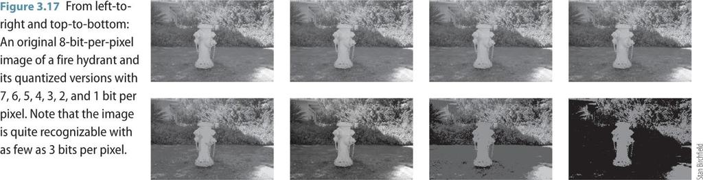
13 Quantization Artifacts False contours associated with quantization are most noticeable in smooth areas These artifacts are obscured in highly textured regions Original image Quantized to 8 levels 13

14 Dither Signal Reduce quantization error by adding uniformly distributed white noise (dither signal) to the input image prior to quantization. Dither hides objectional artifacts. To each pixel of the image, add a random number in the range [-m, m], where m is MXGRAY/quantization-levels. Uniform noise v out 0 thr 255 v in 8 bpp (256 levels) 3 bpp (8 levels) 14

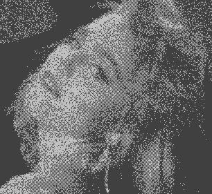
15 Comparison 1 bpp 2 bpp 3 bpp 4 bpp Quantization Dither/ Quantization 15

16 Arithmetic Operations A useful class of graylevel transformations is the set of arithmetic operations, depicted in graphical form in the following figure: 16

17 Saturation Arithmetic Clamp arithmetic operation to lie in [0, 255] range: [ ] = [ ] [ ] = [ ] 17

18 Enhancement Point operations are used to enhance an image. Processed image should be more suitable than the original image for a specific application. Suitability is application-dependent. A method which is quite useful for enhancing one image may not necessarily be the best approach for enhancing another image. Very subjective 18

19 Two Enhancement Domains Spatial Domain: (image plane) - Techniques are based on direct manipulation of pixels in an image Frequency Domain: - Techniques are based on modifying the Fourier transform of an image There are some enhancement techniques based on various combinations of methods from these two categories. 19

20 Enhanced Images For human vision - The visual evaluation of image quality is a highly subjective process. - It is hard to standardize the definition of a good image. For machine perception - The evaluation task is easier. - A good image is one which gives the best machine recognition results. A certain amount of trial and error usually is required before a particular image enhancement approach is selected. 20

21 Piecewise-Linear Transformation Functions Advantage: The form of piecewise functions can be arbitrarily complex Disadvantage: Their specification requires considerably more user input 21

22 Linear Contrast Stretching Low contrast may be due to poor illumination, a lack of dynamic range in the imaging sensor, or even a wrong setting of a lens aperture during acquisition. Applied contrast stretching: (r 1,s 1 ) = (r min,0) and (r 2,s 2 ) = (r max,l-1) 22

23 Linear Contrast Stretching Transformation Linear contrast stretch: A transformation that specifies a line segment that maps gray levels between g min and g max in the input image to the gray levels g min and g max in the output image according to a linear function: 23

24 Linear Contrast Stretching Examples 24

25 Analytic Transformations Graylevel transformations can be specified using analytic functions such as the logarithm, exponential, or power functions: 25

26 Analytic Transformation Examples Linear function - Negative and identity transformations Logarithmic function - Log and inverse-log transformations Power-law function - n th power and n th root transformations 26

27 Image Negatives Negative transformation : s = (L 1) r Reverses the intensity levels of an image. Suitable for enhancing white or gray detail embedded in dark regions of an image, especially when black area is large. 27

28 Log Transformations Log transformation : s = c log (1+r) c is constant and r 0 Log curve maps a narrow range of low graylevels in input into a wider range of output levels. Expands range of dark image pixels while shrinking bright range. Inverse log expands range of bright image pixels while shrinking dark range. 28

29 Example of Logarithm Image Fourier spectrum image can have intensity range from 0 to 10 6 or higher. Log transform lets us see the detail dominated by large intensity peak. - Must now display [0,6] range instead of [0,10 6 ] range. - Rescale [0,6] to the [0,255] range. 29

30 Power-Law Transformations s = cr c and are positive constants Power-law curves with fractional values of map a narrow range of dark input values into a wider range of output values, with the opposite being true for higher values of input levels. c = = 1 identity function 30

31 Gamma Correction (in) γ gamma correction [(in) 1/γ ] γ 1 1 Cathode ray tube (CRT) devices have an intensityto-voltage response that is a power function, with varying from 1.8 to 2.5 This darkens the picture. Gamma correction is done by preprocessing the image before inputting it to the monitor

32 Example: MRI (a) Dark MRI. Expand graylevel range for contrast manipulation < 1 (b) = 0.6, c=1 (c) = 0.4 (best result) (d) = 0.3 (limit of acceptability) When is reduced too much, the image begins to reduce contrast to the point where it starts to have a washed-out look, especially in the background 32

33 Example: Aerial Image Washed-out image. Shrink graylevel range > 1 (b) = 3.0 (suitable) (c) = 4.0 (suitable) (d) = 5.0 (High contrast; the image has areas that are too dark; some detail is lost) 33

34 Graylevel Slicing 34

35 Bit-plane slicing One 8-bit byte Bit-plane 7 (most significant) Bit-plane 0 (least significant) Highlighting the contribution made to total image appearance by specific bits Suppose each pixel is represented by 8 bits Higher-order bits contain the majority of the visually significant data Useful for analyzing the relative importance played by each bit of the image 35

36 Example The (binary) image for bitplane 7 can be obtained by processing the input image with a thresholding graylevel transformation. - Map all levels between 0 and 127 to 0 - Map all levels between 129 and 255 to 255 An 8-bit fractal image 36

37 8-Bit Planes Bit-plane 7 Bit-plane 6 Bitplane 5 Bitplane 2 Bitplane 4 Bitplane 1 Bitplane 3 Bitplane 0 37

38 Hardware LUTs All point operations can be implemented by LUTs. Hardware LUTs operate on the data as it is being displayed. It s an efficient means of applying transformations because changing display characteristics only requires loading a new table and not the entire image. For a 1024x bit image, this translates to 256 entries instead of one million. LUTs do not alter the contents of original image (nondestructive). Refresh memory For display V in (i,j) Lookup table V out (i,j) Display screen

39 Histogram A histogram of a digital image with gray levels in the range [0, L-1] is a discrete function h(r k ) = n k - r k : the k th gray level - n k : the number of pixels in the image having gray level r k The sum of all histogram entries is equal to the total number of pixels in the image. h(r) r 39

40 Histogram Examples 40

41 Count Histogram Evaluation 5x5 image 6 Plot of the Histogram Graylevel Count Pixel value Total 25 Histogram evaluation: for(i=0; i<mxgray; i++) H[i] = 0; for(i=0; i<total; i++) H[in[i]]++; 41

42 Normalized Histogram Divide each histogram entry at gray level r k by the total number of pixels in the image, n p( r k ) = n k / n p( r k ) gives an estimate of the probability of occurrence of gray level r k The sum of all components of a normalized histogram is equal to 1. 42

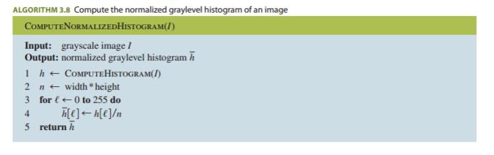
43 Pseudocode 43

44 Histogram Processing Basic for numerous spatial domain processing techniques. Used effectively for image enhancement: - Histogram stretching - Histogram equalization - Histogram matching Information inherent in histograms also is useful in image compression and segmentation. 44

45 Example: Dark/Bright Images Dark image Components of histogram are concentrated on the low side of the gray scale. Bright image Components of histogram are concentrated on the high side of the gray scale. 45

46 Example: Low/High Contrast Images Low-contrast image histogram is narrow and centered toward the middle of the gray scale High-contrast image histogram covers broad range of the gray scale and the distribution of pixels is not too far from uniform, with very few vertical lines being much higher than the others 46

47 Histogram Stretching h(f) h(g) MIN MAX f g 3) Rescale to [0,255] range 1) Slide histogram down to 0 g = 255( f MAX MIN) MIN 2) Normalize histogram to [0,1] range 47

48 Example (1) Wide dynamic range permits for only a small improvement after histogram stretching Image appears virtually identical to original

49 Example (2) Improve effectiveness of histogram stretching by clipping intensities first Flat histogram: every graylevel is equally present in image

50 Histogram Equalization Produce image with flat histogram All graylevels are equally likely Appropriate for images with wide range of graylevels Inappropriate for images with few graylevels (see below) 50

51 Example 51

52 Example (1) before after Histogram equalization 52

53 Example (2) before after Histogram equalization The quality is not improved much because the original image already has a wide graylevel scale 53

54 Implementation (1) No. of pixels x4 image Gray scale = [0,9] histogram Gray level 54

55 Implementation (2) Gray Level(j) No. of pixels k j= 0 n j Cumulative Distribution Function (CDF) s = k j= 0 n j n 0 0 6/16 11/16 15/16 16/16 16/16 16/16 16/16 16/16 s x

56 Implementation (3) No. of pixels Input image Output image Gray scale = [0,9] Gray level Histogram equalization 56

57 Pseudocode 57

58 Why It Works 58

59 Note (1) Histogram equalization distributes the graylevels to reach maximum gray (white) because the cumulative distribution function equals 1 when 0 r L-1 k If n j is slightly different among consecutive k, those graylevels will be j= 0 mapped to (nearly) identical values as we have to produce an integer grayvalue as output Thus, the discrete transformation function cannot guarantee a one-to-one mapping 59

60 Note (2) The implementation given above is widely interpreted as histogram equalization. It is readily implemented with a LUT. It does not produce a strictly flat histogram. There is a more accurate solution. However, it may require a one-to-many mapping that cannot be implemented with a LUT. 60

61 Histogram Equalization Objective Objective: we want a uniform histogram. Rationale: maximize image entropy. h ( v c 1 1 ( v out out ) = constant = ) = h = ( v avg out + 1)* h total MXGRAY This is a special case of histogram matching. Perfectly flat histogram: H[i] = total/mxgray for 0 i < MXGRAY. If H[v] = k * h avg then v must be mapped onto k different levels, from v 1 to v k. This is a one-to many mapping. avg 61

62 Histogram Equalization Mappings Rule 1: Always map v onto (v 1 +v k )/2. (This does not result in a flat histogram, but one where brightness levels are spaced apart). Rule 2: Assign at random one of the levels in [v 1,v k ]. This can result in a loss of contrast if the original histogram had two distinct peaks that were far apart (i.e., an image of text). Rule 3: Examine neighborhood of pixel, and assign it a level from [v 1,v k ] which is closest to neighborhood average. This can result in bluriness; more complex. Rule (1) creates a lookup table beforehand. Rules (2) and (3) are runtime operations. 62

63 Better Implementation (1) void histeq(imagep I1, imagep I2) { int i, R; int left[mxgray], width[mxgray]; uchar *in, *out; long total, Hsum, Havg, histo[mxgray]; /* total number of pixels in image */ total = (long) I1->width * I1->height; /* init I2 dimensions and buffer */ I2->width = I1->width; I2->height = I1->height; I2->image = (uchar *) malloc(total); /* init input and output pointers */ in = I1->image; /* input image buffer */ out = I2->image; /* output image buffer */ /* compute histogram */ for(i=0; i<mxgray; i++) histo[i] = 0; /* clear histogram */ for(i=0; i<total; i++) histo[in[i]]++; /* eval histogram */ R = 0; /* right end of interval */ Hsum = 0; /* cumulative value for interval */ Havg = total / MXGRAY; /* interval value for uniform histogram */ 63

64 Better Implementation (2) /* evaluate remapping of all input gray levels; * Each input gray value maps to an interval of valid output values. * The endpoints of the intervals are left[] and left[]+width[]. */ for(i=0; i<mxgray; i++) { left[i] = R; /* left end of interval */ Hsum += histo[i]; /* cum. interval value */ while(hsum>havg && R<MXGRAY-1) { /* make interval wider */ Hsum -= Havg; /* adjust Hsum */ R++; /* update right end */ } width[i] = R - left[i] + 1; /* width of interval */ } } /* visit all input pixels and remap intensities */ for(i=0; i<total; i++) { if(width[in[i]] == 1) out[i] = left[in[i]]; else { /* in[i] spills over into width[] possible values */ /* randomly pick from 0 to width[i] */ R = ((rand()&0x7fff)*width[in[i]])>>15; /* 0 <= R < width */ out[i] = left[in[i]] + R; } } 64

65 Note Histogram equalization has a disadvantage: it can generate only one type of output image. With histogram specification we can specify the shape of the histogram that we wish the output image to have. It doesn t have to be a uniform histogram. Histogram specification is a trial-and-error process. There are no rules for specifying histograms, and one must resort to analysis on a case-by-case basis for any given enhancement task. 65

66 Histogram Matching C 0 ( v in ) C 1 ( v out ) C 0 ( v out ) h 0 ( v in ) h 1 ( v out ) v in v in v out v out v out =T(v in ) In the figure above, h() refers to the histogram, and c() refers to its cumulative histogram. Function c() is a monotonically increasing v function defined as: c( v) 0 = h( u) du 66

67 Histogram Matching Rule Let v out =T(v in ) If T() is a unique, monotonic function then v out This can be restated in terms of the histogram matching rule: Where c 1 (v out ) = # pixels v out, and c 0 (v in ) = # pixels v in.. This requires that h1 ( u) du = h0 ( u) du which is the basic equation for histogram matching techniques. v in 0 0 c ( vout ) = c0 v ( v 1 in out = c ( c 0 ( v 1 1 in ) )) 67

68 Pseudocode 68

69 Histograms are Discrete Impossible to match all histogram pairs because they are discrete. Refresh memory For display V in (i,j) C 1 ( v out ) Lookup table? V out (i,j) Display screen C 0 ( v in )? v out v in Continuous case v out v in Discrete case 69

70 Problems with Discrete Case The set of input pixel values is a discrete set, and all the pixels of a given value are mapped to the same output value. For example, all six pixels of value one are mapped to the same value so it is impossible to have only four corresponding output pixels. No inverse for c 1 in v out = c 1-1 (c 0 (v in )) because of discrete domain. Solution: choose v out for which c 1 (v out ) is closest to c 0 (v in ). v in v out such that c 1 (v out ) - c 0 (v in ) is a minimum 70

71 Histogram Matching Example (1) Input image Input Histogram Histogram match Output image Target Histogram 71

72 Histogram Matching Example (2) 72

73 Implementation (1) int histogrammatch(imagep I1, imagep histo, imagep I2) { int i, p, R; int left[mxgray], right[mxgray]; int total, Hsum, Havg, h1[mxgray], *h2; unsigned char *in, *out; double scale; /* total number of pixels in image */ total = (long) I1->height * I1->width; /* init I2 dimensions and buffer */ I2->width = I1->width; I2->height = I1->height; I2->image = (unsigned char *) malloc(total); in = I1->image; /* input image buffer */ out = I2->image; /* output image buffer */ for(i=0; i<mxgray; i++) h1[i] = 0; /* clear histogram */ for(i=0; i<total; i++) h1[in[i]]++; /* eval histogram */ 73

74 Implementation (2) /* target histogram */ h2 = (int *) histo->image; /* normalize h2 to conform with dimensions of I1 */ for(i=havg=0; i<mxgray; i++) Havg += h2[i]; scale = (double) total / Havg; if(scale!= 1) for(i=0; i<mxgray; i++) h2[i] *= scale; R = 0; Hsum = 0; /* evaluate remapping of all input gray levels; Each input gray value maps to an interval of valid output values. The endpoints of the intervals are left[] and right[] */ for(i=0; i<mxgray; i++) { left[i] = R; /* left end of interval */ Hsum += h1[i]; /* cumulative value for interval */ while(hsum>h2[r] && R<MXGRAY-1) { /* compute width of interval */ Hsum -= h2[r]; /* adjust Hsum as interval widens */ R++; /* update */ } right[i] = R; /* init right end of interval */ } 74

75 Implementation (3) /* clear h1 and reuse it below */ for(i=0; i<mxgray; i++) h1[i] = 0; } /* visit all input pixels */ for(i=0; i<total; i++) { p = left[in[i]]; if(h1[p] < h2[p]) /* mapping satisfies h2 */ out[i] = p; else out[i] = p = left[in[i]] = MIN(p+1, right[in[i]]); h1[p]++; } 75

76 Local Pixel Value Mappings Histogram processing methods are global, in the sense that pixels are modified by a transformation function based on the graylevel content of an entire image. We sometimes need to enhance details over small areas in an image, which is called a local enhancement. Solution: apply transformation functions based on graylevel distribution within pixel neighborhood. 76

77 General Procedure Define a square or rectangular neighborhood. Move the center of this area from pixel to pixel. At each location, the histogram of the points in the neighborhood is computed and histogram equalization, histogram matching, or other graylevel mapping is performed. Exploit easy histogram update since only one new row or column of neighborhood changes during pixel-to-pixel translation. Another approach used to reduce computation is to utilize nonoverlapping regions, but this usually produces an undesirable checkerboard effect. 77

78 Example: Local Enhancement a) Original image (slightly blurred to reduce noise) b) global histogram equalization enhances noise & slightly increases contrast but the structural details are unchanged c) local histogram equalization using 7x7 neighborhood reveals the small squares inside of the larger ones in the original image. 78

79 79 Definitions (1) = = j i j i y x j i f n y x j i f n y x, 2, )), ( ), ( ( 1 ), ( ), ( 1 ), ( mean standard deviation Let p(r i ) denote the normalized histogram entry for grayvalue r i for 0 i < L where L is the number of graylevels. It is an estimate of the probability of occurrence of graylevel r i. Mean m can be rewritten as = = 1 0 ) ( L i i r i p r m

80 Definitions (2) The nth moment of r about its mean is defined as It follows that: L n ( r) = i= 0 ( r) = 1 ( r) = 0 1 ( r) = L 1 i= 0 ( r i ( r i m) n m) p( r 2 i ) p( r i ) 0 th moment 1st moment 2 nd moment The second moment is known as variance 2 ( r) The standard deviation is the square root of the variance. The mean and standard deviation are measures of average grayvalue and average contrast, respectively. 80

81 81 Example: Statistical Differencing Produces the same contrast throughout the image. Stretch f(x, y) away from or towards the local mean to achieve a balanced local standard deviation throughout the image. 0 is the desired standard deviation and it controls the amount of stretch. The local mean can also be adjusted: m 0 is the mean to force locally and α controls the degree to which it is forced. To avoid problems when (x, y) = 0, Speedups can be achieved by dividing the image into blocks (tiles), exactly computing the mean and standard deviation at the center of each block, and then linearly interpolating between blocks in order to compute an approximation at any arbitrary position. In addition, the mean and standard deviation can be computed incrementally. ), ( )), ( ), ( ( ), ( ) (1 ), ( 0 0 y x y x y x f y x m y x g + + = ), ( )), ( ), ( ( ), ( ) (1 ), ( y x y x y x f y x m y x g =

82 Example: Local Statistics (1) The filament in the center is clear. There is another filament on the right side that is darker and hard to see. Goal: enhance dark areas while leaving the light areas unchanged. 82

83 Example: Local Statistics (2) Solution: Identify candidate pixels to be dark pixels with low contrast. Dark: local mean < k 0 *global mean, where 0 < k 0 < 1. Low contrast: k 1 *global variance < local variance < k 2 * global variance, where k 1 < k 2. Multiply identified pixels by constant E>1. Leave other pixels alone. 83

84 Example: Local Statistics (3) Results for E=4, k 0 =0.4, k 1 =0.02, k 2 =0.4. 3x3 neighborhoods used. 84