A short tutorial for RIDE toolbox

Transcription

1 A short tutorial for RIDE toolbox Guang Ouyang ---- before Sep Department of Physics Hong Kong Baptist University ---- from Sep Institut für Psychologie Universität Greifswald

2 Overview of algorithm modules Procedure Outcome Tips & Cautions Practice

3 Ouyang et al., 2015, Psychophysilology

4 The Procedure export EEG data from your EEG softwares import data into Matlab run RIDE script (several lines) collect the outcome and do the analyses

5 The Procedure export EEG data from your EEG softwares import data into Matlab Brain Product e.g., Neuroscan e.g., etc run RIDE script (several lines) collect the outcome and do the analyses

6 The Procedure export EEG data from your EEG softwares EEGLAB import data into Matlab run RIDE script (several lines) collect the outcome and do the analyses

7 The Procedure export EEG data from your EEG softwares import data into Matlab run RIDE script (several lines) collect the outcome and do the analyses

8 The Procedure export EEG data from your EEG softwares import data into Matlab run RIDE script (several lines) Matlab script (example) cfg = [];%initialization cfg.samp_interval = 2; cfg.epoch_twd = [-200,1200]; cfg.comp.name = {'s','c','r'}; cfg.comp.twd = {[0,600],[100,900],[-300,300]}; cfg.comp.latency = {0,'unknown',rt}; collect the outcome and do the analyses cfg = RIDE_cfg(cfg); results = RIDE_call(data,cfg);

9 The Procedure export EEG data from your EEG softwares import data into Matlab run RIDE script (several lines) collect the outcome and do the analyses

10 About RIDE toolbox RIDE is a package of Matlab code Implementation of RIDE is just a few lines of code. After implement RIDE, the results is saved in data matrix, one can choose: either do all the analysis and plottings in Matlab (require basic Matlab scripting background) or export the data into your favorite softwares (spss) or programming environments (python, R).

11 Start RIDEing add the RIDE package to the Matlab path Create a new m-script and type the following: Configure the separation scheme and parameters cfg = [];%initialization cfg.samp_interval = 2; cfg.epoch_twd = [-200,1200]; cfg.comp.name = {'s','c','r'}; cfg.comp.twd = {[0,500],[100,900],[-300,300]}; cfg.comp.latency = {0,'unknown',rt}; Run cfg = RIDE_cfg(cfg); results = RIDE_call(data,cfg);

12 Time window selection stimulus onset reaction Times trial index ms time S C S for capturing the early, stimuluslocked component, empirically, [0, 500] C for capturing the latency-variable component cluster Time window is selected from the beginning and termination of the hump (see next slide)

13 An example of separating ERP into one C components S C R

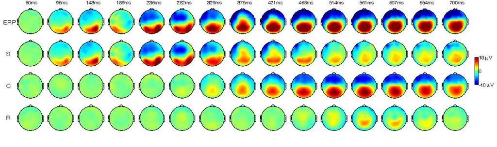
14 Time window selection A general scenario of RIDE separation: (grand averaged ERP) ERP S C R component is set as [ ] around RT assuming that the RTlocked cluster is within this time window. The pattern of the R is in line with the assumption (right). R

15 Data and RT extracting S010 S255 S010 S255 S010 S255 S010 S255 S010 S255 Do not involve nonbrain channels! When data is imported by EEGLAB, the data and event information is stored in EEG.data and EEG.event. We need a few lines of script to extract the RT. We have an example in RIDE_call/example/Snippet for data and rt extraction

16 Data and RT extracting Finally the data prepared like this is ready for RIDE Importance: - data only contain a single subject and single condition - RT matches data trial by trial.

17 Different RIDEing Schemes, for examples: Typical task with RT: S+C+R Nogo trials: S+C Reading task: S+C1(N400) + C2(P600) Extremely simple task: S + R etc..

18 Different RIDEing Schemes Create an new m-script and type the following: S+C+R cfg = [];%initialization cfg.samp_interval = 2; cfg.epoch_twd = [-100,1000]; cfg.comp.name = {'s','c','r'}; cfg.comp.twd = {[0,500],[100,900],[-300,300]}; cfg.comp.latency = {zeros(size(data,3),1),'unknown',rt}; cfg = RIDE_cfg(cfg); results = RIDE_call(data,cfg);

19 Different RIDEing Schemes Create an new m-script and type the following: S+C cfg = [];%initialization cfg.samp_interval = 2; cfg.epoch_twd = [-100,1000]; cfg.comp.name = {'s','c'}; cfg.comp.twd = {[0,500],[100,900]}; cfg.comp.latency = {zeros(size(data,3),1),'unknown'}; cfg = RIDE_cfg(cfg); results = RIDE_call(data,cfg);

20 Different RIDEing Schemes Create an new m-script and type the following: S+C1+C2+R cfg = [];%initialization cfg.samp_interval = 2; cfg.epoch_twd = [-100,1000]; cfg.comp.name = {'s','c1','c2','r'}; cfg.comp.twd = {[0,500],[100,600],[400,900],[-300,300]}; cfg.comp.latency = {zeros(size(data,3),1), 'unknown', 'unknown', rt}; cfg = RIDE_cfg(cfg); results = RIDE_call(data,cfg);

21 Different RIDEing Schemes Create an new m-script and type the following: S+R cfg = [];%initialization cfg.samp_interval = 2; cfg.epoch_twd = [-100,1000]; cfg.comp.name = {'s','r'}; cfg.comp.twd = {[0,500], [-300,300]}; cfg.comp.latency = {zeros(size(data,3),1), rt}; cfg = RIDE_cfg(cfg); results = RIDE_call(data,cfg);

22 An example of separating ERP into one C components S C R

23 An example of separating ERP into two C components C2 S C1 R Principle for C time windows: covering a complete hump for each C

24 After RIDEing Know how to see the results Please refer to the handbook for detailed explanation for all of the meanings of the variables in the outcome

25 The Outcome separated components Time courses Topographies reconstructed ERP single trial variability

26 The outcome (waveforms of separated components)

27 The outcome (waveforms of separated components) ERP S C grand mean R

28 The outcome (topography)

29 The outcome (reconstructed ERP)

30 The outcome (reconstructed ERP)

31 RIDE Outcome: ERP re-construction: conditional effects To solve the smearing effect due to latency variability Case I1. Latency variability reduces the amplitude effect Cond. 1 Cond. 2 Case I2. Different latency variability makes to amplitude effect 9/25/

32 The outcome (reconstructed ERP) What to see? Example: statistical testing on reconstructed ERP

33 The outcome (reconstructed ERP) 9/25/

34 The outcome (reconstructed ERP) 9/25/

35 The outcome (reconstructed ERP) 9/25/

36 The outcome (reconstructed ERP) 9/25/

37 The outcome (variability) [trials 1] [trials electrodes]

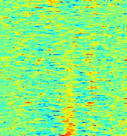
38 The outcome (variability) S C ,000 ms R ,000 ms 20 A B C latency variability trial (sorted by RT) trial (sorted by RT) trial (sorted by RT) lag (ms) lag (ms) lag (ms) D 20 E 20 F amplitude variability trial (sorted by RT) trial (sorted by RT) trial (sorted by RT) V time after stimulus (ms) time after stimulus (ms) time after stimulus (ms)

39 The outcome (variability) Variability information: S C R Amplitude Latency (stimulus onset) Latency amplitude Amplitude Latency (RT) Behavior Individual difference Genetics Diseases

40 Hints and Cautions Data quality The general quality of data is important for the quality of outcome. Be careful of the quality of your data. Better to have a visual inspection of your data before applying RIDE. Examples of bad data

41 Hints and Cautions Why do we separate C component and when it is perhaps not suitable to separate C? - C is clearly visible in the standard ERP stimulus onset 20 reaction Times C1 C2 40 trial index ms time - If a C is not even visible from standard ERP, then RIDE might not be able to extract it. RIDE restores component from blurring, not creating components.

42 An example of separating ERP into two C components C2 S C1 Q: Can I separate a lot of C component clusters? R A: It is technically doable. But it is not recommended. Each C requires a clear template to estimate its latency in single trial. Too many C components will make each template contains too little information. We always keep it as one (or two if visually clear) C component clusters.

43 An example of separating ERP into one C components S C R

44 An example of separating ERP into one C components S C R

45 An example of separating ERP into two C components (two humps) C2 S R C1

46 Hints and Cautions Reduce sampling rate to improve computation speed Sampling rate = 1000 Too high is not necessary And reduce speed Sampling rate = 500 Sampling rate = 250 Above this is OK Sampling rate = 100 Sampling rate = 50

47 Hints and Cautions Do not involve non-brain channels (e.g., M1,M2,VEOU,VEOL,EOG,ECG etc) Clearly remove artifacts, especially serious drifting Observe the grand mean to specify the time windows for RIDE components. More hints and cautions please refer to the manual (cns.hkbu.edu.hk/ride.htm)

48 Go through it RIDE website: cns.hkbu.edu.hk/ride.htm Download: RIDE toolbox Slides of introduction of RIDE Slides of implementation of RIDE RIDE manual Set path: Unzip RIDE toolbox, put the folder RIDE_call in the folder toolbox under Matlab direactory. For example: C:\Program Files\MATLAB\R2014a\toolbox\. Launch Matlab -> set path -> add with subfolders -> choose the folder of RIDE_call -> select folder -> save -> close. Download EEGLAB (for topography ploting) It is also useful to download EEGLAB toolbox (sccn.ucsd.edu/eeglab). Because we need to use the function topoplot from EEGLAB to plot the topography of the results. And besides, EEGLAB is very powerful in EEG data importing from commercial EEG softwares. When adding the EEGLAB toolbox to Matlab, remember to choose add with subfolder rather than add folder.

49 Practice - apply on an single subject in Matlab format - Example of load file from Brain Product and obtain RT information - Example of load file from Neuroscan - Example of batch script - Examples of plotting and basic analysis

50 Practice: apply on an single subject already in Matlab format Load example data (from a single subject, single condition): In Matlab, load (open) the data samp_face.mat under RIDE_call\example\. There are three variables in it data the 3-D matrix (time*electrode*trial) chanlocs the information about channels labels and locations (the is usually obtained by EEGLAB when importing data from commercial softwars) rt the reaction time information (in millisecond) for all single trials. Run RIDE. The script is saved in (..\RIDE_call\example\single_subject.m ). %run the following script in Matlab (select them -> right click -> Evaluation selection cfg = [];%initialization cfg.samp_interval = 2; cfg.epoch_twd = [-100,1000];%time window for the epoched data (relative to stimulus) cfg.comp.name = {'s','c','r'};%component names cfg.comp.twd = {[0,500],[100,900],[-300,300]}; %time windows for extracting components, for 's' and 'c' it is raltive to stimulus, for 'r' it is relative to RT cfg.comp.latency = {0,'unknown',rt};%latency for each RIDE component %Note: you are supposed to know the above information for your own data. %The time windows for RIDE component is from observation of ERP cfg.re_samp = 8; %down sampling to 125 to raise speed (optional) cfg = RIDE_cfg(cfg);%standardize results = RIDE_call(data,cfg); %run RIDE It takes a few minute to run this data..\ride_call\example\single_subject.m

51 Practice: apply on an single subject already in Matlab format Plot the waveform chan_index = find(strcmpi({chanlocs.labels},'cz'));%select which channel to plot %plot erp and RIDE components superimposed together figure;ride_plot(results,{'erp','s','c','r'},chan_index);..\ride_call\example\single_subject.m %or plot the ERP and reconstructed ERP superimposed figure;ride_plot(results,{'erp','erp_new'},chan_index);

52 Practice: apply on an single subject already in Matlab format Plot the waveform %Plot all the time courses for all electrodes together %set the time axis first t_axis = linspace(cfg.epoch_twd(1),cfg.epoch_twd(2),size(data,1)); %plot ERP figure;plot(t_axis, results.erp); axis tight;xlabel('time after stimulus (ms)');ylabel('potential (\muv)'); %you can simply change ERP to S figure;plot(t_axis, results.s); axis tight;xlabel('time after stimulus (ms)');ylabel('potential (\muv)');..\ride_call\example\single_subject.m

53 Plot the topography Practice: apply on an single subject already in Matlab format t = 500;%the time point to plot, in millisecond t1 = round((t-cfg.epoch_twd(1))/cfg.samp_interval);%covert t to sampling point c_range = [-15,15];%specify the color range figure;subplot(1,4,1);topoplot(results.erp(t1,:),chanlocs);text(0,1,'erp');caxis(c_r ange); subplot(1,4,2);topoplot(results.s(t1,:),chanlocs);text(0,1,'s');caxis(c_range); subplot(1,4,3);topoplot(results.c(t1,:),chanlocs);text(0,1,'c');caxis(c_range); subplot(1,4,4);topoplot(results.r(t1,:),chanlocs);text(0,1,'r');caxis(c_range);..\ride_call\example\single_subject.m

54 Practice: apply on an single subject already in Matlab format Plot the topography evolution twd = [100,900];%the time window to be plotted n = 10; %how many topos to be shown comp = {'erp','s','c','r'}; c_range = [-15,15];%specify the color range temp = [];twd_s = round((twd-cfg.epoch_twd(1))/cfg.samp_interval);%convert the sampling point for j = 1:length(comp) eval(['temp{j} = results.',comp{j},'(twd_s(1):twd_s(2),:);']); end t_points = round(linspace(twd(1),twd(2),n)); figure;topos_scr(temp,t_points,comp,chanlocs,'maplimits',c_range);..\ride_call\example\single_subject.m

55 Practice: apply on an single subject already in Matlab format Plot the latency of C versus RT %plot the latency of c versus RT figure;plot(results.latency_c*cfg.samp_interval,results.latency_r*cfg.samp_interval,'.'); xlabel('single trial latency of C (ms)'); ylabel('single trial RT (ms)'); title(['the correlation is ',num2str(corr(results.latency_c(:),results.latency_r(:)))]);..\ride_call\example\single_subject.m

56 Plot single trials Practice: apply on an single subject already in Matlab format %plot single trial ERP chan_index = find(strcmpi({chanlocs.labels},'pz')); t_axis = linspace(cfg.epoch_twd(1),cfg.epoch_twd(2),size(data,1));%time axis; temp = single_trial_ride(data,results,'erp',chan_index); figure;imagesc(t_axis,1:size(data,3),temp');colormap('jet'); xlabel('time after stimulus (ms)'); ylabel('trial index'); %plot single trial S chan_index = find(strcmpi({chanlocs.labels},'o1')); t_axis = linspace(cfg.epoch_twd(1),cfg.epoch_twd(2),size(data,1));%time axis; temp = single_trial_ride(data,results,'s',chan_index); figure;imagesc(t_axis,1:size(data,3),temp');xlabel('time after stimulus (ms)');ylabel('trial index');colormap('jet'); %sort by the accending order of amplitude figure;imagesc(t_axis,1:size(data,3),temp(:,accending_index(results.amp_s(:,chan_index)))' );colormap('jet'); xlabel('time after stimulus (ms)');ylabel('trial index'); %plot single trial C chan_index = find(strcmpi({chanlocs.labels},'pz')); t_axis = linspace(cfg.epoch_twd(1),cfg.epoch_twd(2),size(data,1));%time axis; temp = single_trial_ride(data,results,'c',chan_index); figure;imagesc(t_axis,1:size(data,3),temp');xlabel('time after stimulus (ms)');ylabel('trial index');colormap('jet'); %sort by the accending order of C latency figure;imagesc(t_axis,1:size(data,3),temp(:,accending_index(results.latency_c))'); xlabel('time after stimulus (ms)');ylabel('trial index');colormap('jet');..\ride_call\example\single_subject.m

57 Practice: Example of load file from Brain Product and obtain RT information - eeglab - File --> Import Data --> Using EEGLAB functions and plugins --> From Brain Vis. Rec..vhdr file - After loading the data, the scipt history was saved in EEG.history - Because this data is a mixture of all conditions, we have to separate it into different condition - Open..\RIDE_call\example\Snippet for data and rt extraction\extract_data_and_rt.m - This is an example of how to split the data with mixed condition into a single condition and how to extract RT. - When the data was prepared and RT was extracted, RIDE can be applied like previous.

58 Practice: Example of load file from Neuroscan software - - Download and unzip batch_data_demo.zip from cns.hkbu.edu.hk/ride.htm - Note: this data is already segmented into 3-D in Neuroscan. Each file only contain a single subject and condition. eeglab File --> Import Data --> Using EEGLAB functions and plugins --> From NEUROSCAN.EEG - Randomly select a.eeg file and load it Simply check the artifact: figure;plot(eeg.data(:,:)');

59 Practice: Example of load file from Neuroscan software - Prepare the data in RIDE format and then one can apply RIDE data = permute(eeg.data,[2,1,3]); - Note: there is no RT info for this demo data, so one can only separate S and C - All the relevant info for RIDE should be in principle contained in EEG. - We also need to save the channel location file as a separate.mat file for the ease of following plottings. Usually one can simply run: chanlocs = EEG.chanlocs; and save the chanlocs variable as a.mat file. However, sometimes there is no information contained in EEG.chanlocs, which is probably due to the configuration of exporting process. In this case, one can use EEGLAB to fill those location infomations: edit -> channel locations -> OK -> OK. (but again, this is some issue in this function in some version of EEGLAB ). - After EEGLAB fills the info in the EEG.chanlocs, you can extract and save it: chanlocs = EEG.chanlocs; save('..\chanlocs.mat','chanlocs');

60 Practice: Batch processing! - Here is a demo to prepare a batch for applying RIDE in all subjects and conditons - Download and unzip batch_data_demo.zip from cns.hkbu.edu.hk/ride.htm - Note: this data is already segmented into 3-D in Neuroscan. Each file only contain a single subject and condition. - Run the following batch file and then you can collect all results: con = {'High','Baseline'}; % you have to make this condition names consistent with you data file sub = {'Sub1','Sub2','Sub4','Sub5','Sub7','Sub8','Sub10','Sub11','Sub12',... 'Sub13','Sub14','Sub15','Sub16','Sub17','Sub19','Sub20','Sub21','Sub22','Sub23','Sub24','Sub25','Sub26','Sub29','Sub30'}; % make it consistent with your subject names in your folder/data file data_dir = 'C:\Dropbox\data\jamie\batch_data_demo\'; % the root directory of your data for j = 1:length(sub) for k = 1:length(con) EEG = pop_loadeeg([sub{j},'_',con{k},'.eeg'], [data_dir,sub{j},'\'], 'all','all','all','all','auto'); %this line can be found in EEG.history when you use eeglab to load a single file data = permute(eeg.data,[2,1,3]); cfg = [];%initialization cfg.samp_interval = 4; cfg.epoch_twd = [-104,1936];%time window for the epoched data (relative to stimulus) cfg.comp.name = {'s','c'};%component names cfg.comp.twd = {[0,500],[100,900]}; %time windows for extracting components, for 's' and 'c' it is relative to stimulus, for 'r' it is relative to RT cfg.comp.latency = {0,'unknown'};%latency for each RIDE component cfg = RIDE_cfg(cfg);%standardize results = RIDE_call(data,cfg); save([data_dir,'results_',sub{j},'_',con{k},'.mat'],'results'); end end It takes around one or two hours to finish all the data

61 Practice: plottings and basic analysis - When all the data were processed, it will be saved in your computer - But you can use the result files in batch_data_demo.zip for the following demos for plottings and analysis - Open the grand_plot.m file - First run the script in the first three sections: head, assemble data, grand average (before that you have to change the path name) - You can ignore the section sync R to grand median RT since there is no RT here - Go to the next section plot the separation scenario, you can plot the general scenario of RIDE separation in grand average level - You can change the condition name../batch_data_demo/grand_plot.m

62 Practice: plottings and basic analysis - Run the section plot different components in one figure, you can plot different components or reconstructed ERP super-imposed For left figure: comp = {'erp', 's', 'c'}; For right figure: comp = {'erp','erp_new'};../batch_data_demo/grand_plot.m

63 Practice: plottings and basic analysis - In the following section Plot (grand average) ERP, RIDE-components time courses for different conditions at specific channels, you can compare conditions../batch_data_demo/grand_plot.m

64 Practice: plottings and basic analysis - In the following section, you can plot the map of topography difference.../batch_data_demo/grand_plot.m

65 Practice: plottings and basic analysis - Map evolution (and difference in a later section)../batch_data_demo/grand_plot.m

66 Practice: plottings and basic analysis - Simple t-test on amplitude within certain time window../batch_data_demo/grand_plot.m

67 Practice: plottings and basic analysis - Test on the latency variability../batch_data_demo/grand_plot.m

68 Generalized to other applications - So far you have gone through every steps of RIDE application all the way from data importing to results plottings and analysis. You can, in principle, generalize to other data. There is a step that is not covered, that is, how to set the configurations in commercial EEG softwares when exporting the data. It is required that the data should be artifact removed, epoched into 3d data matrix and separated for each single subject and single condition. But unfortunately I don t have experience on that so I could not give guidance. But a person familiar with ERP experiment should know that quite well. - If you have some basic background about Matlab, it will be easy for you to change the demo script and adapt it to your data. If not, it is also possible to understand it a bit, look up some script from google and ask others for help.

69 Thank you!