SYSTAT A Tutorial Manual. Cover version 12

Size: px

Start display at page:

Download "SYSTAT A Tutorial Manual. Cover version 12"

Jennifer Carson
5 years ago
Views:

1 SYSTAT A Tutorial Manual Cover version 12

2 Table of Contents Table of Contents... ii Introduction to SYSTAT... 1 SYSTAT Basics... 2 Tutorial 1: Starting a SYSTAT Session... 2 Tutorial 2: Getting Help on SYSTAT... 5 Tutorial 3: A Graphic Tour in SYSTAT... 5 Tutorial 4: Ending A SYSTAT Session... 6 Creating and Manipulating Data in SYSTAT... 7 Tutorial 1: Creating a New Data Set... 7 Tutorial 2: Saving a New Data Set Tutorial 3: Creating a New Data Set from Other File Formats Tutorial 4: Opening an Existing SYSTAT Data Set Tutorial 5: Printing a Data Set Generating Descriptive Statistics in SYSTAT Tutorial 1: Mean, Sum, Standard Deviation, Variance, Minimum, Maximum, and Range Tutorial 2: Correlation Generating Graphical Statistics in SYSTAT Tutorial 1: How to Generate Scatter Plots Tutorial 2: How to Generate a Histogram Tutorial 3: How to Generate a Box Plot Statistical Models in SYSTAT Tutorial 1: Linear Regression Tutorial 2: Analysis of Variance Tutorial 3: Test for normality Tutorial 4: Chi-square analysis Statistical Graphics in SYSTAT - by command approach Tutorial 1: Scatter plot Tutorial 2: Scatter plot with two separate graphs overlaid Tutorial 3: More examples ii

3 Introduction to SYSTAT SYSTAT is a statistical software package that calculates basic and advanced statistics. There are two basic ways of implementing procedures in SYSTAT. The easiest way to execute a procedure is by using the menu bars that are located in the SYSTAT Main and Data windows. In this manual, this is how procedures are implemented. However, sometimes it is more helpful to implement a command to perform a procedure. In this case, the commands can be used. We ll cover this aspect in the last session of this manual. The following manual will give an introductory description of how to use SYSTAT version 12. However, due to the complex nature of SYSTAT, many details have been omitted. Some helpful websites concerning SYSTAT are: You are required to consult the specific sections in the manuals to get more detail information. SYSTAT comes with seven electronic volumes of manuals, i.e., Getting Started (412 pages), Data (321 pages), Graphics (512 pages), Language Reference (435 pages), Quality Analysis (50 pages), Statistics (I, II, III, and IV, 2200 pages) and Monte Carlo (78 pages). To read them all may be impossible (4,008 pages!), but you should become familiar with them, especially the data and graphics part. You ll be required in this class to produce scientific graphics using this package in the final project which is a poster presentation. Check Tutorial in the online Help System to get a quick start. 1

4 SYSTAT Basics Tutorial 1: Starting a SYSTAT Session Select Programs from the Start menu. Select SYSTAT from the menu. When a SYSTAT session is started, the following window will appear. The important windows in SYSTAT are: Output Organizer, Dynamic Explorer, Output Pane, Data Editor, Graph Editor and Command Editor. 2

5 3

6 4

Tutorial 2: Getting Help on SYSTAT Select Help from the SYSTAT Main window toolbar. The following window will appear which indicates how to use the Help menu in SYSTAT.

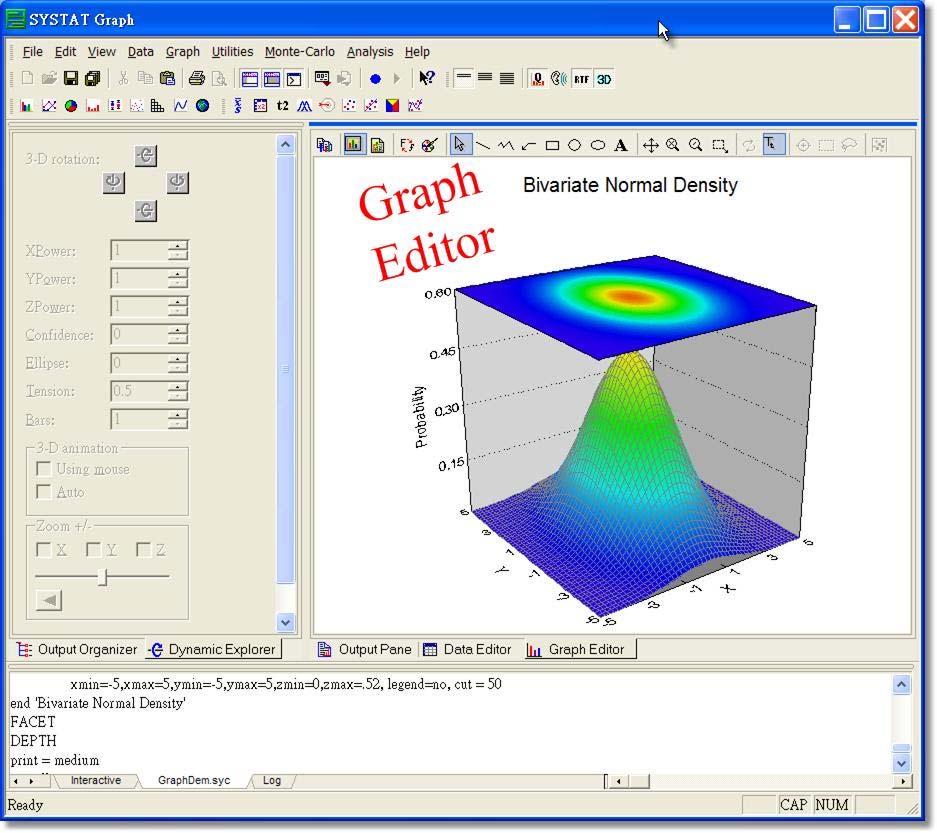
7 Tutorial 2: Getting Help on SYSTAT Select Help from the SYSTAT Main window toolbar. The following window will appear which indicates how to use the Help menu in SYSTAT. This help system provides easy access to some of the most important information when you need them. However, as mentioned before, you should consult the specific sections in the six electronic manuals to get more detail information. Tutorial 3: A Graphic Tour in SYSTAT You can get a first look on what SYSTAT can offer in scientific graphics by executing the command file, GraphDem.syc, located in ~/SYSTAT 12/Command/GraphDemo folder. When you load the file, just use File, submit window to execute the problem. 5

8 Tutorial 4: Ending A SYSTAT Session Select Exit from the File menu on the SYSTAT Main window. 6

Creating and Manipulating Data in SYSTAT Data files in SYSTAT are in the form of a spreadsheet where each row represents a case while each column represents a variable.

9 Creating and Manipulating Data in SYSTAT Data files in SYSTAT are in the form of a spreadsheet where each row represents a case while each column represents a variable. To view, enter, edit, and save data, the Data window is used. Tutorial 1: Creating a New Data Set Problem Enter the following data into SYSTAT. Solution Name Age Weight Mark Allison Tom Cindy From the Window menu, select File, New, Data. The SYSTAT Data window will appear. 7

10 Define the variables of the data SYSTAT recognizes two types of data: string data and numerical data. For variables with string data, the variable name, followed by $, is entered in the appropriate column heading. For variables with numerical data, just enter the variable name in the appropriate column heading. To enter a variable name into a column, left click on the column header and select the Variable Properties to pop-up the window, and type the name of the variable. To move to a new column, left click on the new column. NOTE: Once a column is defined, SYSTAT will not allow changes to the data type. For example, to define the variable, Name, left click on the first column heading, select Variable properties, the Variable Properties windows pop-up. and type Name$. However, to define the variable, Age, left click on the second column heading and type Age. Do this for the variable, Weight, as well. 8

To indicate a cell that does not have a data value, a period

11 Once all variables are defined, enter the data by left clicking on a cell and entering the appropriate information. To indicate a cell that does not have a data value, a period is entered. A period represents a missing value. Window Output 9

12 Use File/Save (Active File, AS, All) or just Save to save your work. Tutorial 2: Saving a New Data Set For example, from the File menu, select Save As This will open the Save A File dialog box. 10

From the Save file as type ( 存檔類型 ) drop-down list, select Systat Files (*.syz, note that the syd or sys extensions are file type for previous SYSTAT version).

13 From the Save file as type ( 存檔類型 ) drop-down list, select Systat Files (*.syz, note that the syd or sys extensions are file type for previous SYSTAT version). From the Folders list, select the path where the file will be saved. In the File Name box, enter a name for the file. SYSTAT automatically adds the extension. Click Save. Tutorial 3: Creating a New Data Set from Other File Formats SYSTAT is able to open files in many formats. These formats include SPSS, Excel, Lotus 1-2-3, dbase, DIF, ASCII files and many more. Problem Read the following file, ~/SYSTAT 12/data/Survey2xls, into a SYSTAT data set. Solution Select Open from the File menu. From the Open drop down list, select Data This will open the Open a File dialog box. 11

14 From the List Files of Type list, select the type of file that will be imported. In this case, select Excel Files (*.xls). In the Folders list, select the path where the file is located. In the File Name box, select the name of the file to be imported. In this case, it is Survey2.xls Click 開啟舊檔. Window Output 12

You can now use save command, as we mentioned previously, to save the file into SYSTAT default format. Tutorial 4: Opening an Existing SYSTAT Data Set Select Open from the File menu.

15 You can now use save command, as we mentioned previously, to save the file into SYSTAT default format. Tutorial 4: Opening an Existing SYSTAT Data Set Select Open from the File menu. From the Open drop down list, select Data This will open the Open a File dialog box. In the Folders list, select the path where the file is located. In the File Name box, select the name of the file to be opened. 13

16 Click OK. Tutorial 5: Printing a Data Set From the Data Editor window, select Print from the File menu. Change the options where appropriate. Click OK. 14

17 Generating Descriptive Statistics in SYSTAT The following tutorials will demonstrate how to generate descriptive statistics in SYSTAT. Tutorial 1: Mean, Sum, Standard Deviation, Variance, Minimum, Maximum, and Range Problem Using the data in the file Admire.syd that is located in ~/SYSTAT 12/data/, determine the mean, sum, standard deviation, variance, minimum value, maximum value, and range for some of the numeric variable. Solution From the Analyze menu on the SYSTAT Main window, select Basic Statistics. This will open the Basic Statistics dialog box. 15

Select N, Mean, Sum, SD, Variance, Minimum, Maximum, Skewness, Kurtosis, and Range from the options. When done, click on the OK button. In the variable list, select Age and Income.

18 Select N, Mean, Sum, SD, Variance, Minimum, Maximum, Skewness, Kurtosis, and Range from the options. When done, click on the OK button. In the variable list, select Age and Income. Click on the Add button to move the variable over to the Variable(s) box. To calculate descriptive statistics for many variables, simultaneously add variables to the Variable(s) box. Click OK. The Basic Statistics dialog box closes and the statistics are output in the SYSTAT Main window. Window Output Note that the values for skewness and kurtosis are all less or close to 1, indicating that the variable is approximately normally distributed. Tutorial 2: Correlation Problem 16 Using the data in the file Cars.syz that is located in ~/SYSTAT 12/data/, determine the correlation between acceleration (ACCEL) and slalom time (SLALOM).

Solution From the Analyze menu on the SYSTAT Main window, select Correlations. From the Correlations drop-down menu, select Simple. This will open the Correlations dialog box.

19 Solution From the Analyze menu on the SYSTAT Main window, select Correlations. From the Correlations drop-down menu, select Simple. This will open the Correlations dialog box. In the variable list, select AGE and INCOME. Left click on the Add button between the boxes to move the variables over to the Variable(s) box. Select the type of correlation to be generated in the Types area. Because this is continuous data, select Pearson as the method to be used. Click on the Options button. This will open the Correlations: Options dialog box. 17

To test that the correlation is 0, the probability of each correlation coefficient is determined by selecting Probabilities. This option will not be used in this case.

20 To test that the correlation is 0, the probability of each correlation coefficient is determined by selecting Probabilities. This option will not be used in this case. To estimate Pearson correlation, covariance, or SSCP matrices from data with missing values, select (EM) Estimation. To identify outliers and to compute the correlation, covariance, or SSCP matrix from the remaining cases, select Hadi outlier identification and estimation. These options will not be used in this case. When done, click on the Continue button. Click OK. The Correlations dialog box closes and the correlations are output in the SYSTAT Main window. Window output 18

21 19

22 Generating Graphical Statistics in SYSTAT The following tutorials introduce how to create scatter plots, histograms, and box plots using the SYSTAT Graph menu located on the SYSTAT Main window menu bar. Here some examples that SYSTAT can create. You can see more by running the demo from GraphDem.syc and the folder at ~/SYSTAT 12/Images/ and ~/SYSTAT 12/Images/Gallery. Tutorial 1: How to Generate Scatter Plots Problem Using the data in ~/SYSTAT 12/data/Aircraft.syz, create an x-y plot of Time and Flutter. 20 Solution

Load the data. From the Graph menu, select Plot and then Scatterplot This will open the Scatterplot dialog box. From the variable list, select the variable, Flutter.

23 Load the data. From the Graph menu, select Plot and then Scatterplot This will open the Scatterplot dialog box. From the variable list, select the variable, Flutter. Left click on the Add button between the variable list and the Y variable(s) box. From the variable list, select the variable, Time. Left click on the Add button between the variable list and the X variable(s) box. Click on the Options menu. There are many different menus that you can choose from. For example, if the Options menu is selected, the dialog box will open. This window will clarify the type of scatterplot to be generated. For more information on each of the options given, check Help. 21

24 22 If the Smoother menu is selected, the Smoother dialog box will open. This window will provide a choice of smoothers that can be used to fit lines to 2-D displays.

25 23 If the Residuals menu is selected, the Residuals dialog box will open. This window will plot the standardized residuals of the dependent variable based on the type of regression chosen.

If the Coordinates menu is selected, the Coordinates dialog box will open. Several types of coordinates and projections are available for appropriate data.

26 If the Coordinates menu is selected, the Coordinates dialog box will open. Several types of coordinates and projections are available for appropriate data. In this case, none of these options are used. Click on the Continue button. Select the X-Axis menu. This will open the X-Axis dialog box. This window gives options concerning the x-axis on the scatter plot to be created. In the Axis label box, enter Time (sec.). 24

27 Select the Y-Axis menu. This will open the Y-Axis dialog box. This window gives options concerning the y-axis on the scatter plot to be created. In the Axis label box, enter Flutter. Open the All Axes dialog menu. This will give options to modify both x and y axes. In this case, no options will be selected. 25

28 26 Click on the Layout menu.

This window will specify the title, the location on the page, and size adjustments for the scatter plot. In this case, the title of the graph is Scatter Plot of Time vs. Flutter.

29 This window will specify the title, the location on the page, and size adjustments for the scatter plot. In this case, the title of the graph is Scatter Plot of Time vs. Flutter. In our case, Legend menu is grey and can t be open. This window provides a key to the symbols, fills, lines, or colors that distinguish the legends. If the Color menu is selected, the Color dialog box will open. This window will allow changes to the color of the scatter plot generated. In this case, no options are selected. 27

30 28 If the Fill menu is selected, the Fill dialog box will open. This window will allow changes to the fill of the scatter plot generated. In this case, no options are selected.

31 29 If the Symbol and Label menu is selected, the Symbol and Label dialog box will open. This window will allow symbols to be used to mark the points on a graphical display. Points can also be labelled. In this case, no options are selected.

32 In our case, the Surface and Line Style menu is in grey, the Surface and Line Style dialog box can t be opened. This window will allow changes to the line style. Click OK. The Scatterplot dialog box closes and SYSTAT activates the SYSTAT Graph dialog box. The chart will be displayed here. Window Output 30

Tutorial 2: How to Generate a Histogram Problem Using the data in ~ /SYSTAT 12/data/Iris.syz, create histogram of SEPALLEN for SPECIES=1, 2, and 3, respectively.

33 Tutorial 2: How to Generate a Histogram Problem Using the data in ~ /SYSTAT 12/data/Iris.syz, create histogram of SEPALLEN for SPECIES=1, 2, and 3, respectively. Solution Open the data file. Before we open the Graph menu, we have to turn on the GROUP. From Data menu, select By Group. Add SPECIES as the grouping variable. 31

Left click on the Add button between the variable list and the X-variable(s) box to move the variable to this box.

34 Click OK. From the Graph menu, select Density Displays, and then Histogram This will open the Histogram dialog box. From the variable list, select the variable, SEPALLEN. Left click on the Add button between the variable list and the X-variable(s) box to move the variable to this box. Click on the Options menu. Similar to the previous tutorial, there are many menus that you can choose from. Some are quite similar to what we have seen. Check the Type of Display option. There are four types to choose from. No change in our case. 32

If the Options menu is selected, the Histogram Options dialog box will open. This window will determine the number and width of the bars of the histogram to be created.

35 If the Options menu is selected, the Histogram Options dialog box will open. This window will determine the number and width of the bars of the histogram to be created. In this case, no options are selected. If the Coordinates menu is selected, the Coordinates dialog box will open. This window will determine the coordinate system (Rectangular or Polar) to use when plotting the histogram. In this case, no options are selected. 33

36 All other menus to be selected are explained in the previous tutorial on scatter plots. Click OK. The Histogram dialog box will close and SYSTAT will activate the SYSTAT Graph dialog box. The histogram will be displayed here. Window Output 34

37 35 You can save the graph by double click any of the graph and open the Graph Editor Window.

38 36 When you press save button, you can save the graph. Save the file as a WMF format will give you the most benefits.

39 Tutorial 3: How to Generate a Box Plot Problem Using the data in the file, ~ /SYSTAT 12/data/Boxes.syz, produce a boxplot of OHMS. Solution From the Graph menu, select Box Plot This will open the Box Plot dialog box. From the variable list, select the variable, income. Left click on the Add button between the variable list and the X-variable(s) box to move the variable to this box. To create box plots for other variables, add the variables simultaneously. Click on the Options menu. This window will determine the appearance of the box plot to be created. In this case, no options are selected. 37

40 38 If the Coordinates menu is selected, the Coordinates dialog box will open. This window will determine the coordinate system to use when plotting the histogram. In this case, no options are selected.

41 All other menus to be selected are explained in the previous tutorial on scatter plots. Click OK. The Box Plot dialog box will close and the box plot will be displayed here. Window Output 39

42 40

43 Statistical Models in SYSTAT Tutorial 1: Linear Regression Problem Using the data in ~/SYSTAT 12/data/Earnbill.syz, compute a least squares regression line to investigate if a person s billing can predict his earning. Solution From the Analysis menu, select Regression. From the Regression drop-down menu, select Linear... and Least square This will open the Regression dialog box. From the variable list, select the variable, BILLINGS. Left click on the Add button between the variable list and the Dependent box to move the variable, BILLINGS, to this box. From the variable list, select the variable, EARNINGS. Left click on the Add button between the variable list and the Independent box to move the variable, height, to this box. 41 Click on the Include constant box to include a constant into the model.

44 Click on the Options button. This will open the Regression: Options dialog box. This window gives options for specifying a tolerance level, selecting complete or stepwise entry, and specifying entry and removal criteria. In this case, since there is only one independent variable, complete estimation will be used. Click on the Continue button when done. Click OK. The Regression dialog box closes and the results of the analysis is found in the SYSTAT Main window. The SYSTAT Graph window will also open with a residual plot. Window Output 42

45 43

Tutorial 2: Analysis of Variance Problem Using the data in ~/SYSTAT 12/data/Iris.syz, test if the mean length of petal (PETALLEN) of three iris species is the same.

46 Tutorial 2: Analysis of Variance Problem Using the data in ~/SYSTAT 12/data/Iris.syz, test if the mean length of petal (PETALLEN) of three iris species is the same. Solution From the Analysis menu, select Analysis of Variance (ANOVA). From the ANOVA dropdown menu, select Estimate Model This will open the ANOVA: Estimate Model window. From the variable list, select the variable, PETALLEN. Left click on the Add button between the variable list and the Dependent(s) box to move the variable, PETALLEN, to this box. 44

From the variable list, select the variable, SPECIES. Left click on the Add button between the variable list and the Factor(s) box to move the variable, SPECIES, to this box.

47 From the variable list, select the variable, SPECIES. Left click on the Add button between the variable list and the Factor(s) box to move the variable, SPECIES, to this box. To determine which pairs of means differ significantly, select the type of post hoc test that will be used. In this case, try Tukey. To save residuals and other data to a new data file, click on the Save file box and select which type of data to be saved. In this case, this option will not be used. Click OK. The ANOVA: Estimate Model dialog box closes and the results of the analysis are found in the SYSTAT Main window. The SYSTAT Graph window will also open with a residual plot. Window Output 45

48 46

Tutorial 3: Test for normality Problem Using the data in ~/SYSTAT 12/data/Iris.syz, test if the lengths of petal (PETALLEN) of three iris species are normally distributed.

49 Tutorial 3: Test for normality Problem Using the data in ~/SYSTAT 12/data/Iris.syz, test if the lengths of petal (PETALLEN) of three iris species are normally distributed. Solution From the Data menu, select By Group. Use SPECIES as the variable. From Analysis menu, select Descriptive statistics and Basic statistics. Add PETALLEN to the Selected variable. From the Options, pick skewness and kurtosis. Press OK. The following results are for: SPECIES =

50 PETALLEN N of cases 50 Minimum Maximum Mean Standard Dev Skewness(G1) Kurtosis(G2) The following results are for: SPECIES = PETALLEN N of cases 50 Minimum Maximum Mean Standard Dev Skewness(G1) Kurtosis(G2) The following results are for: SPECIES = PETALLEN N of cases 50 Minimum Maximum Mean Standard Dev Skewness(G1) Kurtosis(G2) Then, use Graph, Density Plot and Histogram to plot the histogram for the PETALLEN of the three species. Here are the results: The following results are for: SPECIES =

51 Count Proportion per Bar PETALLEN The following results are for: SPECIES = Count Proportion per Bar PETALLEN The following results are for: SPECIES =

52 Count Proportion per Bar PETALLEN You can judge the data normality based on the skewness and kurtosis values. The rule of thumb is that if these two values are within -1 and 1, then it is approximately normal. You can also visually inspect the histogram to see the distribution of these values. We ll talk about specific test later in class. Tutorial 4: Chi-square analysis Problem Let s create a date-file and call it Student.syz. This data file can be created using Excel and imported into SYSTAT. This is how the data looked AFTER in the worksheet: 50

53 And this is the summary table (this is not the form we want): Our problem is to test if the sexes among the different majors are independent. Solution 51

54 From the Analysis menu, select Tables. From the Tables menu, select Two way This will open the Two-way Table window. Next add Major to the Row variable and Gender to the Column: And then check "OK". You will get output that will contain information similar to the following: 52

55 53 The χ 2 value is with DF=3. The result is highly significant.

Statistical Graphics in SYSTAT - by command approach SYSTAT provides programming language that allows you to generate efficient statistics and graphics easily.

56 Statistical Graphics in SYSTAT - by command approach SYSTAT provides programming language that allows you to generate efficient statistics and graphics easily. When performing your analysis using point and click approach, SYSTAT actually generate commands that conduct the analyses. You can check these commands at the Command window by pressing the Log. Sometimes it is necessary to save these commands for future reference, such as to check for potential errors and to redo the graphics. Tutorial 1: Scatter plot Problem We use the data used by Lee et al. (1993) to generate a scatter plot of body weight distribution trend of male and female flying squirrel (Petaurista petaurista) from Taiwan. 54

57 Lee, P. F., Y. S. Lin, and D. R. Progulske Reproductive biology of the red-giant flying squirrel, Petaurista petaurista, in Taiwan. Journal of Mammalogy 74: Solution Here is the command: USE "C:\REPROD1.SYS" REM -- Following commands were produced by the ORDER dialog: ORDER MONTH$ / SORT=NONE DATA REM -- End of commands from the ORDER dialog REM -- Following commands were produced by the PLOT dialog: PLOT MALE FEMALE*MONTH$ / OVERLAY XLABEL = 'Month' YLABEL = 'Body Weight (g)' YMAX = 1500 YMIN = 1200 AXES=L HEIGHT = 2.6 WIDTH = 4.2 LEGEND=NONE FILL=1,0 SYMBOL=1,1 REM -- End of commands from the PLOT dialog This is done by performing a similar Graphing point-and-click process that we introduced in previous tutorial. The graph looks like this: 1500 Body Weight (g) Dec. Jan. Feb. Mar. Apr. May Jun. Month Jul. Aug. Sep. Oct. Nov. 55

58 Tutorial 2: Scatter plot with two separate graphs overlaid Problem In Figure 1 of Lee et al. (1993), carefully check the error bars in both male and female under each month. They made a mistake by placing the same value for each sex. Here are the commands used to generate the figure in the old SYSTAT version 5.0: 56 REM Reproduction figure 1, revised to include SE type=british use c:\reprod1 begin thick=1 orign=0.2in, 2.7in cplot Female * Month$ /Line,symbol=2, fill=1, axes=2, size=1.2, ymin=1200, ymax=1500, error1=femalese, xlabel='', ylabel='', height=2.6in, width=4.2in, stick, nsort orign=0.2in, 2.7in cplot Male * Month$ /Line,symbol=2, fill=0, axes=2, size=1.2, ymin=1200, ymax=1500, error1=femalese, xlabel='', ylabel='',

59 height=2.6in, width=4.2in, stick, nsort thick=4 origin = 0.0in, 0.0in write 'Month'/x=2.4in, y=2.2in, center, width=0.14in, height=0.18in write 'Body Weight (g)'/ x=-0.5in,y=4.1in, center, angle=90, width=0.16in, height=0.13in end quit Check the red mark. This is how the mistake came from. If we want to correct the problem using SYSTAT version 12, what should we do? Solution The original data file should be OK to read into SYSTAT because it was in SYSTAT s format. However, the commands need to be revised as follows: Version 1 USE "C:\REPROD1.SYS" REM -- Following commands were produced by the Data/ORDER dialog: ORDER MONTH$ / SORT=NONE DATA BEGIN LINE MALE*MONTH$/ DIRECTION=MaleSE ERROR=MaleSE, YMAX = 1500 YMIN = 1200, HEIGHT = 5.2 WIDTH = 8.2 COLOR=10, XLABEL = 'Month' YLABEL = 'Body Weight (g)' AXES=L, LINE FEMALE*MONTH$/ DIRECTION=FemaleSE ERROR=FemaleSE, YMAX = 1500 YMIN = 1200, HEIGHT = 5.2 WIDTH = 8.2 COLOR=10, AXES=NONE, SCALE=NONE END Note the use of Begin and End which can combine several graphs into a single figure. In the above case, we combine two figures. Here is the new figure: 57

60 1500 Body Weight (g) Dec. Jan. Feb. Mar. Apr. May The above graph does not have the symbols. So we produce a new one as follows. Jun. Month Jul. Aug. Sep. Oct. Nov. Version 2 USE "C:\REPROD1.SYS" REM -- Following commands were produced by the Data/ORDER dialog: ORDER MONTH$ / SORT=NONE DATA BEGIN DOT MALE*MONTH$/ Line DIRECTION=MaleSE ERROR=MaleSE, YMAX = 1500 YMIN = 1200, AXES=L, HEIGHT = 5.2 WIDTH = 8.5, COLOR=10 FILL=0 SYMBOL=1, XLABEL = 'Month' YLABEL = 'Body Weight (g)' DOT FEMALE*MONTH$/ Line DIRECTION=FemaleSE ERROR=FemaleSE, YMAX = 1500 YMIN = 1200, AXES=NONE SCALE=NONE, HEIGHT = 5.2 WIDTH = 8.5, COLOR=10 FILL=1 SYMBOL=1 END And the figure: 58

61 1500 Body Weight (g) Dec. Jan. Feb. Mar. Apr. May Except for the font and some cosmetic appearance, the graph looks quite similar to the original figure 1. Most importantly, it is a correct figure. Jun. Month Jul. Aug. Sep. Oct. Nov. Tutorial 3: More examples Below are some examples taken from the paper by Ding et al. (2005) that will be published in Global Ecology and Biogeography. Ding, T. Z., H. W. Yuan, S. Geng, Y. S. Lin, and P. F. Lee Energy, body size, and diversity in relation to bird species richness along an elevational in Taiwan. Global Ecology and Biogeography 14: (in press) Figure 2 Commands 59 USE "c:\ys_regr.syz" begin plot BSR*ELEV / LOC=0cm,15cm axes=l scale=l symbol=1 fill=1, size=1.5 YTICK=4 SMOOTH=quadrat SHORT, XMIN=1000 XMAX=4000 ymin=0 ymax=40 xlabel='', ylabel='bird species richness' height=4cm width=6cm plot DEN*ELEV / LOC=7.7cm,15cm axes=l scale=l symbol=1 fill=1, size=1.5 YTICK=4 SMOOTH=quadrat SHORT,

62 XMIN=1000 XMAX=4000 ymin=0 ymax=80 xlabel='', ylabel='total density' height=4cm width=6cm plot Energy_CNSM*ELEV / LOC=0cm,10cm axes=l scale=l symbol=1, fill=1 size=1.5 YTICK=4 SMOOTH=linear SHORT, XMIN=1000 XMAX=4000 ymin=0 ymax=8000 xlabel='', ylabel='energy flux' height=4cm width=6cm plot NPP*ELEV / LOC=7.7cm,10cm axes=l scale=l symbol=1 fill=1, size=1.5 YTICK=4 SMOOTH=linear SHORT, XMIN=1000 XMAX=4000 ymin=0 ymax=2000 xlabel='', ylabel='net Primary Productivity' height=4cm width=6cm write 'Elevation (m)' / LOC=5.5cm,8.8cm, width=0.4cm height=0.4cm write '(a)' / LOC=0.5cm,18.5cm, width=0.4cm height=0.4cm write '(b)' / LOC=8.2cm,18.5cm, width=0.4cm height=0.4cm write '(c)' / LOC=0.5cm,13.5cm, width=0.4cm height=0.4cm write '(d)' / LOC=8.2cm,13.5cm, width=0.4cm height=0.4cm end Graph 40 (a) 80 (b) Bird species richness Total density Energy flux (c) Net Primary Productivity (d) Elevation (m) 60 Figure 3

63 Commands: USE "C:\ys_regr.SYZ" begin origin=4cm,-21.5cm plot BSR*NPP / LOC=0cm,15.5cm, axes=box fill=1, symbol=1 size=1.5 YTICK=4, SMOOTH=quadrat SHORT, XMIN=0 XMAX=1500 ymin=0 ymax=40, xlabel='net Primary Productivity', ylabel='bird Species Richness', height=4cm width=6cm plot ENERGY_CNSM*NPP / LOC=7.7cm,15.5cm, axes=box fill=1, symbol=1 size=1.5 YTICK=4, SMOOTH=linear SHORT, XMIN=0 XMAX=1500 ymin=0 ymax=6000, xlabel='net Primary Productivity', ylabel='energy Flux', height=4cm width=6cm plot DEN*ENERGY_CNSM / LOC=0cm,10cm, axes=box fill=1, symbol=1 size=1.5 YTICK=4, SMOOTH=quadrat SHORT, XMIN=0 XMAX=6000 ymin=0 ymax=80, xlabel='energy Flux', ylabel='total Density', height=4cm width=6cm plot BSR*DEN / LOC=7.7cm,10cm, axes=box fill=1, symbol=1 size=1.5 YTICK=4, XMIN=0 XMAX=80 ymin=0 ymax=40, SMOOTH=linear SHORT, xlabel='total Density' ylabel='bird Species Richness', height=4cm width=6cm write '(a)' / LOC=0.5cm,18.7cm width=0.4cm height=0.4cm write '(b)' / LOC=8.2cm,18.7cm width=0.4cm height=0.4cm write '(c)' / LOC=0.5cm,13.3cm width=0.4cm height=0.4cm write '(d)' / LOC=8.2cm,13.3cm width=0.4cm height=0.4cm write 'r =0.70' / LOC=3.5cm,16cm width=0.3cm height=0.3cm write '2' / LOC=3.6cm,16.2cm width=0.2cm height=0.2cm write 'r =0.71' / LOC=11.2cm,16cm width=0.3cm height=0.3cm write '2' / LOC=11.3cm,16.2cm width=0.2cm height=0.2cm write 'r =0.91' / LOC=3.5cm,10.5cm width=0.3cm height=0.3cm write '2' / LOC=3.6cm,10.7cm width=0.2cm height=0.2cm 61

64 write 'r =0.67' / LOC=11.2cm,10.5cm width=0.3cm height=0.3cm write '2' / LOC=11.3cm,10.7cm width=0.2cm height=0.2cm end Graph Bird Species Richness (a) 2 r =0.70 Energy Flux (b) 2 r = Net Primary Productivity Net Primary Productivity Total Density (c) 2 r =0.91 Bird Species Richness (d) 2 r = Energy Flux Total Density Figure 4 Commands: USE "c:\ys_regr.syz" plot M_BAR*Energy_CNSM / LOC=3.5in,10in axes=box scale=l, symbol=1 fill=1 size=1, SMOOTH=quadrat SHORT, height=6in width=6in XTICK=4 YTICK=5, XMIN=0 XMAX=6000 ymin=0 ymax=150, xlabel='total Energy Flux', ylabel='individual Consumption' end Graph 62

65 150 Individual Consumption Total Energy Flux With some exercises and practices, you should be happy to work with SYSTAT when you want to produce publication-quality graphics. SYSTAT s example command files There are over 500 examples in the seven volumes or five volumes (if we count Statistics I, I and III as one volume) of the SYSTAT User Manual. The input commands for each example in the User Manual or in the Help system are available as command files in the ~/SYSTAT 12/Command/ folder of the installed directory. This provides an alternative way to run the examples. These files are organized in terms of the printed manual. Each file contains commands for one example and is named using six characters (xxyyzz.syc). The first two characters represent the corresponding volume of the printed manual as follows: 63 'da' for Data ('DataVolume' in the folder) 'gs' for Getting Started ('Getting_Started' in the folder)

66 'gr' for Graphics ('Graphics' in the folder) 's1' for Statistics I ('Statistics_I' in the folder) 's2' for Statistics II ('Statistics_II' in the folder) 's3' for Statistics III ('Statistics_III' in the folder) 's4' for Statistics III ('Statistics_IV' in the folder) The next two digits represent the chapter number within the volume, and the last two digits represent the example number within the chapter. These files are organized in the 'Command' folder with 11 subfolders, seven of them corresponding to the seven volumes mentioned above. Two additional subfolders, 'GraphDemo' and 'Miscellaneous', contain commands of examples which are not numbered. The names of files in the 'Miscellaneous' folder are indicative of the examples they relate to. For example, to execute the commands given in Example 1 in Chapter 2 of Statistics III, submit the 's30201.syc' file. To run these commands, you may have to define paths appropriately. Good luck and happy computing. 64

1. Basic Steps for Data Analysis Data Editor. 2.4.To create a new SPSS file

1 SPSS Guide 2009 Content 1. Basic Steps for Data Analysis. 3 2. Data Editor. 2.4.To create a new SPSS file 3 4 3. Data Analysis/ Frequencies. 5 4. Recoding the variable into classes.. 5 5. Data Analysis/