ACT-R Environment Manual

Transcription

1 Working Draft Dan Bothell

2 Table of Contents Table of Contents...2 Preface...3 Introduction...4 Running the Environment...6 Environment Overview...9 Current Model...11 Model...13 Control...15 Current Data...30 Recorded Data...44 Miscellaneous Window Positions and Sizes Extending or Changing the Environment Available Environment Extras Standalone Environment Tools Advanced Issues

3 Preface This document is a work in progress to describe the operation of the ACT-R Environment. The content is accurate, but may not cover all the components of the Environment. It may also make reference to sections or other documents which are not yet available. The hope is that although it is not yet complete, this working version will be of some use to ACT-R modelers. 3

4 Introduction The ACT-R Environment is a GUI written in Tcl/Tk which can be connected to ACT-R to help users with running, inspecting, and debugging models. It also provides a way to display a GUI with which a model is interacting for Lisps which don t have such capabilities, and for the standalone versions of ACT-R (pre-built applications which run without needing to have a Lisp in which to run ACT-R) it also provides some basic text editing capabilities for model files. This document assumes the user has a basic understanding of ACT-R. [If you do not, then you should probably start with the ACT-R tutorial.] It will focus primarily on running the Environment in conjunction with ACT-R running in a separate Lisp application. All of the same tools are available when running the standalone version, and the documentation on the additional Environment tools included with the standalone version of ACT-R is included in the Standalone Environment Tools section. To generate the information displayed by the Environment it uses the same ACT-R commands that are available to the user when using ACT-R from a command line. Thus, for the most part, it does not provide anything new for working with ACT-R. However, because it displays the command outputs in separate windows and updates those windows as the model runs it can be a lot easier to use when debugging, and for some things, like the buffer traces and BOLD response predictions, it displays the data graphically instead of just textually. 4

5 Requirements There are a few requirements necessary to run the ACT-R Environment: - You need to have the ACT-R software. - If you are using Windows or Mac OS X then you can use the pre-built Environment application which is included with the distributions. - If you are not using Window or Mac OS X or if you prefer not to use the pre-built Environment application, then you will need a wish interpreter to run the Environment from the Tcl/Tk source code which is included in all the ACT-R software distributions. It should run in any Tcl/Tk version 8.1 or newer, but or newer is recommended. - The Lisp in which you run ACT-R must have the ability to open and communicate via TCP/IP sockets, it must have multiprocessing capabilities, and there must be an appropriate ACT-R interface for those Lisp capabilities. The distribution includes interfaces for Allegro Common Lisp, LispWorks, Clozure Common Lisp, CMUCL, and SBCL. If your Lisp has the necessary capabilities but is not one of those, it is possible to extend the ACT-R interface to include it (see the Adding Lisp Support section under advanced topics). - You will need to have TCP functionality on your machine, but it s not necessary to have an active internet connection as long as you are going to run the Environment and ACT-R on the same machine. 5

6 Running the Environment This section assumes that you are loading ACT-R into a supported Lisp application. If you are using a standalone version of ACT-R then you should consult the documentation which came with it as to how to run that. The Environment runs as a separate application from the Lisp in which ACT-R is running. It communicates with ACT-R via a TCP/IP socket connection and can be run on the same machine or a different machine than the Lisp running ACT-R. It is also possible to have more than one Environment connected to the same ACT-R session. In this section the assumption will be that there is one Environment connection occurring on the same machine which is running the Lisp with ACT-R. For details on other situations (remote connections and multiple concurrent Environments) see the advanced sections. Standard Method Here are the standard steps to follow to run ACT-R with the Environment on all systems (there is a shorter alternative for some Lisp and OS combinations covered later): 1. The first thing to do is load ACT-R into your Lisp application (see the ACT-R reference manual for details). 2. Start the Environment application. a. If you are using one of the pre-built applications ( Start Environment.exe on Windows or Start Environment OSX on Macs) run it like you would any other application. Note: if you are using Mac OS 10.8 or newer and get an error dialog indicating that the file is "damaged and can't be opened" the issue is probably due to permissions. Open your System Preferences and under "Security & Privacy" set the "Allow applications downloaded from:" to Anywhere, and then try running it again. If it successfully runs, then you can change your preferences back to a safer setting. b. If you are using Linux/Unix or do not want to use the prebuilt applications 6

7 then you can run the Environment from the source files. To do so you must have Tcl/Tk installed (Linux and OS X often have it installed automatically). Then, all you need to do is either execute the starter.tcl script found in the environment/gui directory or you can use wish (the Tcl/Tk interpreter) to run it i.e. "wish starter.tcl". 3. Once the Environment is running you should have seen a Powered by ONR splash screen briefly and then have a window titled Control Panel open which says Waiting for ACT-R at the top. 4. To connect ACT-R to the Environment you need to call the start-environment function in Lisp. 5. That should result in another splash screen opening briefly to show the ACT-R version information and then the Waiting for ACT-R message should be removed from the Control Panel window and several buttons should appear there instead. Once the buttons appear the Environment is ready to use. When you are done using the Environment you should close the connection from the Lisp by calling the stopenvironment function. That should put the Control Panel back into the waiting state. At that point you can close the Environment application if you want, or you can leave it running to connect to again when you need it. You should only close the Environment application (the Control Panel window) when it is in the waiting state. Simplified Method If you are using Clozure Common Lisp or Allegro Common Lisp under Mac OS X, Windows, or Linux or are using LispWorks under either Mac OS X or Windows, then you may be able to replace the steps above with these steps: 1. The first thing to do is load ACT-R into your Lisp application (see the ACT-R reference manual for details). 7

8 2. Call the run-environment function from Lisp. That should automatically run the appropriate Environment application and then initiate the connection between ACT-R and the Environment. If the Environment application does not start, then you should use the standard instructions described above. If the Environment application is slow to start and there is an Unable to connect message displayed in the Lisp you can ignore those and wait for it to try again. If that happens regularly and you want to avoid the unable to connect warnings, then you can increase the delay before ACT-R attempts to connect to the Environment. The delay can be provided as an optional parameter to run-environment indicating how many seconds to wait before connecting. The default delay is 5 seconds. A longer delay may be necessary in some cases, and on some machines a shorter delay will work just fine. 8

9 Environment Overview Once it is connected the Control Panel should look similar to the image below. The appearance will vary based on which operating system you are using, but all of the same components should be available. 9

10 The Control Panel consists primarily of buttons which open the tools that it provides. Those buttons are grouped into sections based on their functions. Each section of the Control Panel and its buttons will be described below. Note that there is a scroll bar on the right of the control panel and some of the buttons may not be visible without scrolling the window or making it larger. One thing to note about the Environment is that it was originally designed to work with a single ACT-R model at a time. It has recently been extended to allow all of the tools to work when there are multiple models currently defined within the default meta-process (it still does not work with multiple meta-processes). Details on using the Environment with multiple models can be found in the Current Model section below If you encounter any problems with using the Environment please contact Dan (db30@andrew.cmu.edu) with the details. 10

11 Current Model The Current Model section has only one item which is a button that serves two purposes. The text shown on the button displays the name of a currently defined model or the text No Current Model if there is no model currently defined. By default, the Environment assumes that there will only be one model defined at a time and the tools will always work with the currently defined model, if there is one. Thus, if a different model is loaded to replace the current one the open inspector windows will then begin working with that new current model. Multiple Models It is possible to use the environment with multiple simultaneously defined models. To enable that, the Allow the environment to work with multiple models option needs to be set (see the Options section). When there are multiple models simultaneously defined the button will still show the name of a single model. With multiple model support enabled, when an Environment tool is opened it will always be associated with the model that was current when it was initialized and that model name will be shown in the title of the tool. To change which model is current, press the button which shows the current model. That will bring up a menu with all of the currently available models in it. That would look like this if there were three models named count, addition, and semantic defined: The one with the checkmark next to the name is the one currently being used, and clicking on one of the other names will switch that model to the current one in the Environment. Because the tools are associated with specific models when there are multiple models defined those tools will become unusable if that model is no longer available and trying to 11

12 use one may result in warnings or problems within the Lisp running ACT-R. There is an options setting which will cause the inspector tools for models which are no longer available to be closed automatically, but that is not always desirable for a couple of reasons and by default the option is disabled. Probably the strongest reason for not enabling the switch is that when clear-all gets called it deletes all the current models which means loading a model file which contains a clear-all will result in closing all the inspector windows. The Reload button in the environment is sensitive to that and if that button is used to reload a model it will not close the inspector windows if the option is enabled, but any other reloading of the model file will e.g. calling the reload function from Lisp. 12

13 Model The model section contains controls for working with model files. When using the Environment with a Lisp running ACT-R it will have only one button which is described in the next section. The standalone version of the Environment has some additional buttons which provide access to a simple text editor. Details on those buttons can be found in the Standalone Environment Tools section later in the manual. Load Model The Load Model button can be used to load a model file into Lisp. This button will open a file selection dialog and the file which is chosen will be loaded into the Lisp running ACT-R. If the compile definitions option of the Environment is enabled, then that file will be compiled and loaded. After loading the file a dialog window will be opened to show any output, warnings, or errors which occurred during the load. If the load completed successfully then it will say Successful Load at the top of the dialog like this: If there is a problem it will indicate that by saying Error Loading at the top like this: 13

14 In either case, the Ok button on the resulting dialog should be pressed to close the dialog before doing anything further with the Environment. This button will only work if the Environment is running on the same machine as the Lisp running ACT-R. Also, if the Lisp you are using has a menu or other easy to use mechanism for loading and compiling files then you should use that instead of this button because that is likely to provide much better handling of errors or other unusual circumstances. 14

15 Control The control section contains buttons for stepping through the trace of running models, for viewing the events that are scheduled, and for restoring the models to their initial conditions. Reset The Reset button is used to return models to their initial state. Pressing the Reset button is equivalent to calling the ACT-R reset command. Reload The Reload button is used to load the last model file which was loaded into the Lisp again (a model file is defined as a file which calls the ACT-R clear-all command at the top-level in the file). Pressing the Reload button is equivalent to calling the ACT-R reload command. The Reload button will not function if ACT-R is currently running or if the Stepper tool is open, In those cases it will open a dialog to indicate that: That dialog should be closed by pressing the Ok button before continuing with any of the other tools. Stepper The Stepper button is perhaps the most useful tool in the Environment. When it is pressed it will open the Stepper if it is not already open. If it is open, then pressing this button will bring it to the front there can be only one Stepper open in the Environment 15

16 even if there are multiple models defined. The Stepper is used to step ACT-R through its execution one event at a time. The Stepper looks like this when you first open it: To use the stepper you must have it open before you start the model running. If you try to open it while the model is currently running it will display a dialog like this indicating that it is unavailable: 16

17 Thus, the proper way to use it is to open the Stepper and then call the appropriate function to run the model from Lisp. If you close the Stepper while the model is running the model will continue to run to its natural completion from that point. Stepper operation When the Stepper is open it will pause ACT-R before every event that will be printed in the trace. That means if the :v parameter is set to nil in the model the stepper will not have any events over which to step. By default, if all the currently defined models have :v set to nil when the stepper is opened it will open a dialog box like the following one to indicate that before the Stepper tool opens, but that warning can be disabled in the options: The event which is about to occur will be displayed in the stepper after the Next Event: heading, and for some events, additional information will be displayed in the windows below that. ACT-R is suspended at that point and the modeler may use any of the 17

18 Environment s other tools at that time to investigate the currently defined models. The model will execute the displayed event once the user either presses one of the buttons along the top of the Stepper or closes the Stepper. The details of what the buttons do and the additional information available for some events will be described below. Note that when the Stepper is initially opened the three buttons which will advance the system are disabled. They only become enabled and useable while ACT-R is running. Step The Step button allows the system to continue operation. It will execute the Next Event which is displayed and ACT-R will continue to run to the next event which will be handled by the Stepper, if there is one. This is the button that is most often used with the Stepper it steps the system through its operation one event at a time. Stop The Stop button will stop the current run after it executes the event displayed. There are two important things to note about the Stop button. First is to emphasize that the Next Event shown will be executed by the model when the button is pressed there s no clean way to prevent an event from occurring once it has been stepped to. The other is that it only stops the current run. If the system is being run from Lisp code which contains multiple calls to one of the ACT-R running functions then the system may continue to be run by the next call from that code after the Stop button is pressed i.e. the Stepper s Stop button does not affect the Lisp code which may be providing an experiment or other interface for the model or models. Run Until The Run Until: button works in conjunction with the two interface items to its right which are a selection menu and a text entry box. Pressing the Run Until: button will execute the Next Event and allow the model to run without being paused by the Stepper until the condition specified by the combination in the selection menu and text entry box 18

19 occurs. There are three options for the selection menu: time, production, and module. That choice determines what should be entered into the text entry box. If an invalid value is entered into the text entry box when Run Until: is pressed then a warning will be printed in the trace indicating the issue and the system will be paused at the next available event as if the Step button had been pressed. Here are the details for specifying each of the options for Run Until. Time When Time is selected the text entry box should have a number entered into it which represents the ACT-R time in seconds when the Stepper should next pause the system. If that time has already passed then the model will pause on the next event as usual. If there is no event at that specific time, then the system will be paused at the first event after that time. Production When Production is selected the text entry box should have the name of a production entered into it. The system will then be allowed to run until the next time that named production is either selected or fired. If there are multiple models defined then the system will step until the next time any of those models selects or fires a production of that name. Module When Module is selected the text entry box should have the name of a module entered into it. The system will then be allowed to run until the next event which is generated by that named module. As with the production option, if there are multiple models defined then it will step to the first event generated by the specified module regardless of which model generated that event. There are two things to be careful of with the module option. The first is that the 19

20 module s actual name is required. Some modules have the same name as their buffer, like goal and imaginal, but others do not, for example the module which controls the manual buffer is named :motor. That brings up the other issue. Some modules use a keyword for a name, but the prefixed colon doesn t actually show up in the trace when printing the module s name the :motor module s events only show motor in the trace. To see the list of all the modules true names you can use the ACT-R all-module-names command. Additional Information The bottom portion of the stepper will show detailed information for three specific events within a model: the declarative module s retrieved-chunk, the procedural module s production-selected, and the procedural module s production-fired. For all other events the Stepper detail windows will be blank. Retrieved-chunk When a retrieved-chunk event occurs the stepper will fill in the lower boxes like this (taken from a run of the fan model from unit 5 of the ACT-R tutorial): 20

21 The upper-right pane, labeled Retrieval Request, shows the request which was made to the declarative module that initiated this retrieval. The upper-left pane, labeled Possible Chunks, shows the list of chunks which matched the request. They are ordered based on their activations with the highest activation, and thus the chunk which is retrieved, at the top. Selecting a chunk in this list will cause the lower two panes to be filled with the information appropriate for that chunk. The lower-right pane, labeled Chunk, displays the standard ACT-R printout of the selected chunk. The lower-left pane, labeled Chunk Parameters, will be empty unless 21

22 the subsymbolic computations are enabled for the model. If they are enabled, then that pane will display the declarative memory parameters for the selected chunk as reported by the sdp command. Production-selected When a production-selected event occurs and the Tutor Mode box is not checked (see below for details when it is) the Stepper will look like this (taken from a run of the building sticks task in unit 7): 22

23 The upper-left pane, labeled Possible Productions, shows the list of productions which matched the current state during the last conflict-resolution event. They are ordered based on their utilities with the highest utility, and thus the production which was selected, at the top. Selecting a production in this list will cause the other panes to be filled with the information appropriate for that production. The lower-right pane, labeled Production, displays the text of the production. The lower-left pane, labeled Production Parameters, will be empty unless the subsymbolic computations are enabled for the model. If they are enabled, then that pane will display the procedural parameters for the selected chunk as reported by the spp command. 23

24 The upper-right pane, labeled Bindings, shows all of the variables used in the production and the value that they have while matching the current state. Production-fired When a production-fired event occurs the stepper will look like this (which is the production-fired event that follows the production-selected event shown above): The displays are similar to those for the production-selected event. Now however, only the production which fired is listed in the upper-left pane. The Bindings and Production 24

25 Parameters panes display the same information for that production which they did for the production-selected event. The information in the lower-right pane differs in that now it shows the instantiation of the production instead of the production text. The production s instantiation displays the production text with the variables replaced with their corresponding bindings. Tutor Mode The Tutor Mode check box is for use with the models in unit 1 of the ACT-R tutorial. When the box is checked the Stepper requires additional interaction from the user to continue past a production-selected event. Instead of displaying the production and its bindings for such an event the production is displayed with all of its variables highlighted and the bindings unset like this (from the count model in unit 1 of the tutorial): 25

26 The user is then required to click on each of the highlighted variables and enter the appropriate binding. When one of the variables in the Production pane is clicked a new dialog opens in which the binding should be entered: 26

27 If the correct value is given then the Tutor Response dialog will close and it will replace the variable in the display and the value will be shown under the bindings: If an incorrect answer is given then it will indicate that the entry is incorrect and wait for another value to be entered: 27

28 The two buttons at the bottom of the Tutor Response dialog will provide additional information to help the user get the correct answer. Hint Hitting the Hint button will display a suggestion in the Tutor Response dialog indicating which other tool in the Environment may be used to help find the correct answer: Help Hitting the Help button will print the correct answer in the Tutor Response dialog: 28

29 Event Queue The Event Queue button is used to see all of the events in the current ACT-R metaprocess. When it is pressed it will open the event queue window if it is not already open. If it is open, then pressing this button will bring it to the front there can be only one event queue window open in the Environment even if there are multiple models defined because all of the models are executing within the same meta-process. It shows the output from the mp-show-queue and mp-show-waiting commands, which displays all of the events that are currently scheduled and those which are waiting for some other event to trigger their scheduling. Only the events marked with a * at the start of the line will be displayed in the model s trace with the current parameter settings, and thus be available to the Stepper if in use. 29

30 Current Data The Current Data section of the Control Panel contains buttons for viewing detailed information about particular components of a model in its current state. These buttons can be useful in conjunction with the Stepper to view the details before and after an event occurs. The contents of the windows opened by these tools are automatically updated as the model runs. However, if the model is running at full speed i.e. not in real time and without the Stepper open, then the windows may not be able to refresh fast enough and the contents could lag behind the running model. Even in real time mode, if there are a lot of Current Data tools open they may start to fall behind the current model state. Declarative The declarative tool allows the user to inspect the chunks in a model s declarative memory. Pressing the Declarative button opens a new declarative window for inspecting the declarative memory of the currently selected model and any number of such windows may be open at the same time. This is what a declarative viewer will look like (from the count model in unit 1 of the tutorial): 30

31 The list on the left shows all the chunks in declarative memory by default (see filter below for how to change that). Selecting one of those chunks will then cause the details of that chunk to be displayed in the window on the right: The chunk will be printed in the window, and if the subsymbolic computations are enabled then the window will also show the chunk s parameters as reported by sdp at the top. Filter At the top of the window is a filter which allows one to restrict the display to only chunks which have a particular set of slots. The default of none means that all chunks in declarative memory will be displayed. To change the filter, click on the box containing the current filter value. That will open a window which contains lists of all the different sets of slots which exist among the chunks in declarative memory. If you pick a set of slots from that list that will be displayed in the filter and only chunks which contain that set of slots will be displayed. Here are the available sets of slots for the count model: 31

32 Here is the result of selecting the (start end) set of slots: Why not? The Why not? button at the top of the declarative window can be used to get information about whether a chunk was retrieved or not during the last retrieval request the model made. Pressing the Why not? button will open another window and display the results of calling the ACT-R whynot-dm command for the currently selected chunk in 32

33 the declarative viewer. The Whynot window will display the last retrieval request the declarative memory module received and then display the details of the selected chunk and indicate whether or not it matched that request. Here is a Whynot display for the chunk b.1 seconds into the run (after the model makes its first retrieval request): Here is a Whynot window showing result for the chunk c at that same time: 33

34 Procedural The procedural tool allows the user to inspect the productions in the model s procedural memory. Pressing the Procedural button opens a new procedural window for inspecting the productions of the currently selected model and any number of such windows may be open at the same time. This is what a procedural viewer will look like (from the count model in unit 1 of the tutorial): 34

35 The list on the left contains all of the productions in the model. Selecting one of those productions will cause the details of that production to be displayed in the window on the right: 35

36 The production s text will be printed in the window, and if the subsymbolic computations are enabled then the production s parameters from spp are displayed at the top of the window. Why not? The Why not? button at the top of the procedural window is an important debugging aid. Pressing the Why not? button will open another window and display the results of calling the ACT-R whynot command for the currently selected production in the procedural window along with some other relevant information. The Whynot window will display the time at which the whynot was generated and whether or not the LHS of that production currently matches. If it does match, that will be followed by the instantiation of the production. If it does not match, then it will print the text of the production and indicate the first condition which did not successfully match. Here is a Whynot display for the start production in the count model at the beginning of 36

37 the run when it matches: Here is a Whynot window showing the increment production at that same time which does not match: 37

38 Buffer Contents The buffer contents tool allows the user to inspect the chunks in the currently selected model s buffers. Pressing the Buffer Contents button opens a new buffer window for inspecting the buffer chunks and any number of such windows may be open at the same time. This is what a buffer contents window will look like: 38

39 The list on the left shows the names of all the buffers in the model. Selecting a buffer from that list will cause the title of the window to change to show the buffer being displayed and to show the contents of that buffer in the window on the right. If the buffer is empty then it will print that: If there is a chunk in the buffer, then that chunk will be displayed using the buffer-chunk command (this is from the count model in unit 1 of the tutorial): 39

40 Buffer Status The buffer status tool allows the user to inspect the results of the queries which can be made through the currently selected model s buffers. Pressing the Buffer Status button opens a new buffer status window for inspecting the buffer queries and any number of such windows may be open at the same time. This is what a buffer status viewer will look like: 40

41 The list on the left of the window shows the names of all of the buffers in the model. Selecting a buffer from that list will cause the title of the window to change to show the buffer status being displayed and then show the results of the buffer-status command for that buffer on the right: The buffer-status command shows the queries available for the buffer along with whether or not that query is currently true (t) or false (nil). Visicon Pressing the Visicon button will open a window showing the information currently available to the currently selected model s vision module. Only one such window will exist in the Environment for each available model. If a visicon window is already open for the current model, then pressing the button will bring that window to the front. The visicon window displays the information returned by the print-visicon command and here is an example using the sperling model from unit3 of the tutorial: 41

42 Audicon Pressing the Audicon button will open a window showing the information currently available to the currently selected model s audio module. Only one such window will exist in the Environment for each available model. If an audicon window is already open for the current model, then pressing the button will bring that window to the front. The audicon window displays the information returned by the print-audicon command and here is an example using the sperling model from unit3 of the tutorial: Parameters Pressing the Parameters button will open a window showing all of the currently defined modules and their parameters. Each time the button is pressed a new parameter viewer window will be opened for the current model. Selecting a module from the list will then display all of that module s parameters in a list on the right, and selecting one of those 42

43 parameters will display the current setting of that parameter, the default setting, and any documentation which the module provides for the parameter at the bottom of the window: Unlike the other Current Data tools the parameter viewer does not update as the model runs, but it will update if the parameter is selected again. That is because typically the model parameters are set at the start of a run and not changed during the run. 43

44 Recorded Data The Recorded Data tools provide a way for the user to have ACT-R record detailed information as the model runs (effectively any of the things which can be displayed as the model runs using the Current Data tools) and then be able to inspect that data after the model stops using tools that allow one to view the data at particular times during the run. They also provide a way to save that recorded data to a file so that it can be loaded and inspected at a later time if desired (even without the model itself being available). Select Data Pressing the Select Data button will open a window which allows one to select which information will be recorded for the currently chosen model in the Environment. Only one such window will exist in the Environment for each available model. If a select data window is already open for the current model, then pressing the button will bring that window to the front. Here is an example of a select data tool: 44

45 There are two columns of checkboxes for selecting the information to record. The column on the left contains all of the different types of information which can be recorded. Checking a box next to one will cause the model to store that information while it runs (that will result in the setting of the necessary parameters for the modules involved to record that information). The column on the right lists all of the buffers available in the current model. By default, all of the buffer which are used in productions of the current model will be selected, but one can deselect those or add others as desired (this also causes the :traced-buffers parameter to be set to the list of selected buffers). The information selected in the left column will only be recorded for those buffers which are selected on the right where appropriate e.g. the text trace is recorded for all events regardless of the buffers selected. The settings for what to record will be applied to the model when it is reset as long as the select data window is open, and that also indicates which playback tools to provide for the current model. If the window is closed then the model s parameters will be restored to their default values (or the values set in the model itself) the next time the model is reset. If some of the underling parameters are already set 45

46 in the model then they will be shown as already selected when this window is opened. Save Currently Recorded Information The Save Currently Recorded Information button at the bottom of the select data window can be used to record the model s saved information to a file which can be loaded later for inspection. Pressing the button will open a new file dialog window where you can choose the name of the file in which to save the data. The name and file extension may be anything, but because the data is saved as a Lisp readable file a Lisp source extension (.lisp,.lsp, or.cl) might be a reasonable choice. If the data is successfully saved then a dialog window will open indicating where it was successfully saved: The Ok button in that window should be pressed to close it before using any of the other Environment tools. If there is an error while saving the data then a window will be opened showing the error which occurred: 46

47 Again, the Ok button should be pressed to close the window before using other Environment tools. Recording the information as a model runs requires additional resources. The model will take longer to run the more types of information that are being recorded, and there will be additional computer memory required to store that information. Therefore one probably doesn t want to always record everything, especially once the model is working and it s being run repeatedly to generate results. Also, the size of the save files can be significant for a model that has a lot of data recorded and/or runs for a long time. As an example, the zbrodoff model from unit 4 of the tutorial uses most of the modules in a model and running one block of the task covers 540 seconds of model time. It takes about 6 seconds to run one block on my computer without recording any information. Turning on all of the traces for all buffers increases the time it takes to run one block to about 60 seconds, and the saved data file after that run is approximately 42MB in size. The largest time cost for recording data in this model (and presumably most models) is for the buffer history information. With everything except for that enabled it only takes about 24 seconds to run. View Data Pressing the View Data button will open a window which allows one to access the tools which are available for inspecting recorded model data, either from the current model or from a saved file. Every time the button is pressed a new View Data window will be opened and each one may be used to inspect a different source of recorded data. Here is an example of a view data window: 47

48 At the top are two buttons which allow one to select the data source to be inspected. Below that it indicates the currently chosen data source and the name of the model from which it came, or if there is no currently available source of data it will indicate that like this: By default the window will open with the current model as the data source. Below the data source information are two columns of buttons for the tools that can be used to view the recorded information. The column on the left has tools for general model trace information and those on the right are tools for more specific information. If a button is not enabled it means that the data necessary to use it is not currently being 48

49 recorded for the current model or was not saved in the data file if saved data is being viewed. Current Pressing the Current button in a View Data window will make the Current Model as indicated on the Control Panel the source of data for the tools. If one changes the data that is being recorded for the current model with the Select Data tool then pressing the Current button will be necessary to update the buttons available in the View Data window. Load Saved Pressing the Load Saved button will open a file selection dialog where one can choose a file that was saved using the Save Currently Recorded Information button. If a valid file is chosen then that data will be loaded into ACT-R (which may take some time if the data file is large), the tools in this View Data window will access that data, and the source information in the View Data window will be updated to reflect the file that was loaded as shown here: If there is an error while loading the file a dialog will open indicating there was a problem with some additional information about the error like this: 49

50 If that happens you will have to press the Ok button in that dialog to continue and the View Data window will not change the current source of information it is using. Recorded Data Tools All of the remaining buttons in the View Data window will open new tools to display the recorded data. Each tool will be described in detail below, but there are some common elements to the tools which will be described here. Window Titles When a new tool window is opened it will display the data source in the title of the window. If that source is a current model then it will display the name of the model like this for a tool displaying data for the count model: If saved data from a file is the source then the name of that file will be displayed: Parameters Any parameters which control the display of information in a tool (like :graphic-column- 50

51 widths or production-color) will be saved along with the other data when the Save Currently Recorded Information button is pressed. Those recorded values will be used when the data is loaded from that saved file, and there is currently no way to change them at that point. Individual Tools The sections below will describe the operation of the tools available in the View Data window. Graphic Trace (h.) and Graphic Trace (v.) The Graphic Trace tools provide a graphical representation of a model s operation showing activity for the buffers similar to how the alternate text buffer trace displays information. The two tools work similarly and only differ in the orientation of the data (horizontal or vertical). Pressing the Graphic Trace (h.) button will open a new horizontal Graphic Trace window for the current data source and pressing the Graphic Trace (v.) button will open a new vertical Graphic Trace window for the current data source. Any number of either type of window may be open at any time. When opened, the window will look like this: 51

52 There will be no information displayed in the window until the Get trace button is pressed. Pressing that button will display the recorded trace information with each traced buffer showing its activity in a row or column of the display. Here are the horizontal and vertical traces from running the count model from unit 1 of the tutorial: 52

53 For a long trace it may take some time for the display to be fully drawn. While the display 53

54 is being drawn the word Busy will be shown in the lower left corner of the window, and it will display the word Done in the lower left corner (as seen above) once it finishes drawing the trace. The + and - buttons at the bottom of the window can be used to zoom in or out on the trace. Pressing the + button for that display will zoom in and result in this display for the horizontal trace shown above: Pressing the - button a few times results in this display which may be more useful for a model that runs a long time: 54

55 Each row of the horizontal trace or column of the vertical trace corresponds to one of the buffers in the model. The time runs along the bottom of the horizontal trace and along the left edge of the vertical trace. Boxes in a row or column indicate a time period during which that particular buffer reports that its module was busy, and typically represents the module s processing of a request. The text in the box shows the name of the chunk in the buffer (if there is one) for all of the buffers except the production buffer. The production buffer shows the name of the production which fired at that time. There are a couple of exceptions however in the text displayed. The first is for the buffer named production in the trace. That does not represent a real buffer in the model but instead represents when the procedural module fires productions. The text in those boxes is for the name of the production which was selected and fired during that time. Note that some actions may complete instantaneously (like the goal buffer at time 0) in which case the chunk name will be printed to the right of (or below) the line indicating the activity. If the trace is larger than the window the scroll bars along the edges of the trace can be used to scroll the display, or the Range: boxes at the bottom of the window can be used 55

56 to restrict the trace to a particular segment of the run. To restrict the display to a particular range of the trace times may be entered into both of the boxes. The times are measured in seconds and the first box must have a time less than the time entered into the second box. Then the Redisplay button must be pressed to have the trace redrawn. Here is the count model from above restricted to the time between.1 and.2 seconds in the trace: Placing the mouse cursor over a box in the trace will cause some additional details to be shown in the bottom of the display. In the lower left corner it will show the length of the box in seconds followed by the start and stop times. Also, it will fill in the three sections labeled Request, Chunk, and Notes if there is data for them. The Request section will show the specification of the request which was provided to the buffer which generated the activity in the module if there was one (for the production buffer that will be the name of the production). The Chunk section will show the name of the chunk in the buffer if there is one. The Notes section will display any notes which are associated with that action. By default, only production actions have notes which indicate any! 56

57 output! actions which the production executed, but it is possible to add code to the model to provide additional notes for any buffer as described below. Here is what the display looks like with the mouse positioned over the first retrieval activity in the count model trace: and here is an example with the mouse placed over the second instance of the increment production being fired: 57

58 Sometimes, it s not important to see the text details in the boxes of the trace, for example when zooming out on a large trace to get a more general view for what is happening in the model. In cases like that hitting the Remove Text button will clear the text and show only the boxes. Here is a trace of a run of the zbrodoff model from unit 4 of the tutorial zoomed out to see a couple of trials of the task with the text removed: 58

59 Hitting the Redisplay button will redraw the window and restore the text if desired. Similarly, the Remove Grid button will eliminate the grid lines with the time information from the display. Here is the same trace without both the text and grid: 59

60 The other two buttons on the graphic trace window are for saving an image of the data from the trace. Save 1P The Save 1P button can be used to save an image of the graphic trace as an Encapsulated PostScript file. Pressing that button will bring up a file creation dialog in which you must provide the name for the file in which to save the data. The image will be saved as a single page graphic which contains the whole trace, or the currently displayed range if one is specified. Encapsulated PostScript files can be imported in many applications which are used for word processing and generating presentations. Save Multi. The Save Multi. button can be used to save an image of the graphic trace as a 60

61 PostScript file. Pressing that button will bring up a file creation dialog in which you must provide the name for the file in which to save the data. The image will be saved as a multiple page document, and for the horizontal trace the page is generated in landscape mode. Additional Activity Details Clicking the mouse on an activity box in the graphic trace window will open a more detailed information tool for that action if such data was recorded. For the retrieval buffer it will open a Retrievals window, for the production buffer it will open a Production Grid window, and for all other buffers it will open a Buffers window. Only one such window will be opened per buffer, and clicking on a different box of activity will update the information in the previously opened window. Changing the Display Options There are commands and parameter settings in ACT-R which can be used to control what gets displayed in the graphic trace and configure how things are displayed. Those options are described in the following sections. Buffer widths For the vertical trace the widths of the columns can be specified using the :graphiccolumn-widths parameter in the model (it must be set before the model is run and data is recorded). There is no corresponding setting for the horizontal trace. That parameter can be set to a list of numbers where each number represents the width in pixels of the corresponding column in the trace. If there are fewer numbers specified than there are buffers (columns), then the remaining ones are drawn in the default width. There is no restriction in the setting of how wide the trace can be drawn. Here is a vertical trace of the count model with the following settings in the model: (sgp :graphic-column-widths ( )) 61

62 Buffer Colors By default, the colors chosen for each column (or row) are taken from a predefined list of colors. However, it is possible to specify a particular color for each column or row. Like the :graphic-column-widths parameter described above, the :buffer-trace-colors parameter can be set to a list of color designators and those colors will be used for the columns. A color designator is a Lisp string which is either 4, 7, or 10 characters long. It must start with the character # and the remaining items represent three hexadecimal values for the red, green, and blue value of the color. Each of the color components can be specified using either 1, 2, or 3 hex digits (depending on the color depth desired) and they all must have the same number of digits. Thus, fully saturated red could be specified as #F00, #FF0000, or #FFF Any combination of red, green and blue values may be given in a particular color designator, but the actual color displayed will depend on the monitor and video capabilities of the machine. 62

63 Here is a horizontal trace from the count model with this setting in the model: (sgp :buffer-trace-colors ("#0F0" "#00FFFF" "#FFF000FFF")) Production Colors In addition to being able to control the color of each buffer column or row, for the production boxes it is possible to specify a particular color for each production. If no color is given to a production then it is drawn in the color specified for the production column or row i.e. that is the default color for a production. To specify a color for a production you need to setf the production-color value of the production s name to a color designator (as described above for the buffer colors). For example, to set the color for a production named increment you would add something like this to the model after the definition of the production: 63

64 (setf (production-color 'increment) "#a80") Here is the trace of the count model with that setting and no change to the :buffer-tracecolors parameter: Adding custom Notes The ACT-R add-buffer-trace-notes command can be used to place additional notes into the buffer trace. It takes two parameters which are the name of a buffer and something to store in the trace (it can be anything). It adds that note to the buffer trace at the time which it is called. When the mouse is placed over a box in the graphic trace tools, if there are any custom notes which have been added for that buffer during the time the box covers, then the last such custom note is printed in the Notes: section using a ~a argument in a format call. 64

65 Adding custom notes is something which would most likely occur in the module s request processing code to make that additional information available, but it could be called from the user code or perhaps from one of the event hook functions as well. Here is the display of the count model with the cursor over the first retrieval action with this event added to the model: (schedule-event.075 (lambda () (add-buffer-trace-notes 'retrieval "Extra Info."))) Production Graph Pressing this button opens a new Production Graph window for the current data source and any number of those windows may be open. The tool provides a graph of the production transitions which occurred in the model run. Here is a display of the window without any data shown (how it will always appear upon opening): 65

66 To display the data you need to press one of the seven data display buttons: All Transitions, Frequencies, Cycles, Unique Cycles, Runs, Unique Runs, or Utilities. All of the buttons work similarly, but each provides a slightly different view of the data. The similar operation will be described first, and then the specific details of each will be discussed. After pressing one of the data display buttons the window will show the word Busy in the lower-left corner and all of the controls will be disabled. When it completes it will show the data, print the word Done in the corner, and the buttons will be available again. Here is the display after running the count model from unit 1 of the tutorial and pressing the All Transitions button: 66

67 The display will be a state chart diagram for the productions in the model indicating the order in which they were selected and fired. Each production in the model will be drawn in a box. If the border of the box is black then that production was selected and fired at some time during the run of the model for which the data was recorded. If the box border is gray then that production was not selected and fired. [If the Hide unused productions box is checked before pressing a data display button then the gray boxes will not be displayed.] The box with the green highlight indicates the first production which was selected during the data period being displayed and the box with the red highlight was the last one selected. The arrows indicate the sequencing of the productions. An arrow from 67

68 a production A to a production B means that production B was in the conflict set after production A fired. If the arrow is a solid black line then production B was selected and fired after production A, but if the arrow is dashed and gray then production B was not selected and fired even though it did match the current state. Below the display it will show which type of graph is being displayed along with how many different graphs are available (which can differ based on the button pressed to display the data) and which one of those is currently being shown. When there is more than one graph available the + and - buttons allow you to change which of those available graphs is shown. The differences between the displays for each button will be described next and examples for most will be shown for running the paired model from unit 4 of the tutorial using the command (paired-task 1 4). The All Transitions button will always show only one graph. It will contain all of the transitions which occurred in the production data which was recorded. That data may involve multiple cycles in the graph (a loop which passes through a production multiple times) and there is nothing in the display to separate different cycles. Here is what that shows for the paired task: 68

69 Pressing the Frequencies button will display the same graph as is shown for All Transitions except that the thickness of the links will indicate their relative frequencies with thicker lines being more frequent. Here is the result of that from the example run: 69

70 Pressing the Cycles button will break the data up into one display for each cycle which 70

71 occurs (and possibly an incomplete cycle at the end if it does not form a loop). For each of the cycles displayed it will also show the model s time at the start and end of that cycle at the bottom of the window. Here are two of the cycles from the example run: The Unique Cycles button works similar to the Cycles button, except that it only provides one copy of each different cycle which occurs in the data and does not provide the timing information. In the example run there are only 3 unique cycles among the 4 cycles of the data. The Runs button will break the data up into graphs based on when one of the ACT-R running commands is called, and will provide a separate graph for each run during which at least one production selection occurred. It will show the start and stop times for that run at the bottom of the display. Here are two of the Runs graphs from the example: 71

72 The Unique Runs button works similar to the Runs button, except that it only provides one copy of each different run which occurs in the data and does not provide the timing information. In the example run there are only 3 unique runs among the 8 runs which occurred. The Utilities button works similar to the Runs button except that the data is broken into graphs based on when the model receives rewards. Each reward marks the end of a graph, and there may be one additional graph at the end which does not represent a reward being presented if the model has fired additional productions after receiving the last reward. The display for the Utilities graph is slightly different than the others. First, all of the productions are represented in boxes of the same width instead of being sized based on the production names. In addition to that, each production box may have a blue bar displayed along both the top and bottom of the box. Those bars represent the relative utility of that production (the true utility not counting any noise which may have occurred during the run). The bar along the top represents the utility prior to the reward being provided and the bar along the bottom represents the utility after the reward has been propagated. The utilities are scaled across all productions and all graphs so that the 72

73 maximum utility which any production has is represented by a bar which fills the box from left to right. Here is an example showing part of the graph after running the building sticks learning model from unit 6 of the tutorial. On this trial we can see that the forceover production was selected among the strategy selection productions and that its utility went up when read-done provided a reward. The Save as.eps button at the bottom of the display can be used to save an image of the current production graph as an Encapsulated PostScript file. 73

74 The Save as.dot button at the bottom of the display can be used to save a text description of the currently displayed graph in DOT format for use with Graphviz or other purposes. There is one minor issue currently with the DOT files and that is that the frequency graphs do not currently include any information about the link thickness. Thus, the DOT file for the frequency graph will look exactly like the DOT file for the all transitions graph. Production text For all of the graphs, if you click on the name of a production in the display then it will open a new window displaying the text of that production. Here is an example from clicking the increment production in a graph of the unit 1 count model: Display adjustments There are two parameters which can be set in the model to adjust the spacing of the productions in the display. The :p-history-graph-x parameter specifies the horizontal pixel spacing between the production boxes in a row and defaults to 40. That also determines the maximum thickness of a link for the Frequencies display which will be ¼ 74

75 of the horizontal spacing. The :p-history-graph-y parameter specifies the vertical spacing between rows of productions and defaults to 90. Text Trace Pressing this button opens a new Text Trace window for the current data source and any number of those windows may be open. The tool allows one to see the event trace generated by the model as it ran even if that trace was not being displayed during the run. Here is a display of the window without any data shown (how it will always appear upon opening): To display the data you need to first select the detail level desired with the radio buttons 75

76 on left. The first three options, low, medium, and high, correspond to the setting of the :trace-detail parameter which can be set in a model. The last option, ALL, provides additional information beyond the high detail trace. Selecting all will display every event which occurred, including those which were marked as having no output (which are typically internal system maintenance events like deleting a chunk that is no longer needed or modifying a module s internal data after performing an action). After selecting a detail level the Get Trace button must be pressed. When that button is pressed the window will show the text Waiting... while the trace is being constructed: Once that completes the display will be updated to show the trace information: 76

77 The From and to boxes at the top can be used to restrict the trace to a particular time range. They can be specified as times in seconds, and when the Get Trace button is pressed only events which occur within that time range will be displayed. If the From box is left empty the default is time 0, and if the to box is empty the default is the end of the recorded time. Here is the same trace as shown above restricted to the time between. 1 and.27 seconds: 77

78 Production Grid Pressing this button opens a new Production Grid window for the current data source and any number of those windows may be open. The tool works similar to the horizontal and vertical buffer tracing tools described above. Here is a display of the window without any data shown (how it will always appear upon opening): 78

79 To display the data you need to press the Get history button in the lower-left corner of the window. While the data is being generated the window will show the word Busy in the lower-left corner and the other controls will be disabled. When it completes it will show the word Done in the corner and the buttons will be available again. Here is the display after running the count model from unit 1 of the tutorial: 79

80 The left column displays all the names of the productions in the model, one per row, and if you click on the name of a production then it will open a text window which will contain the text of that production. To the right of the production names there is a column for each time that there was a conflict-resolution event in the model with the time of that event listed at the top (times increasing to the right). By default each conflict-resolution event will have a column. However, you can check the Hide empty columns box at the bottom of the window which will cause it to redraw the graph with the empty columns removed. Here is that same display after checking the Hide empty columns box: 80

81 The color of the cell for a production s row in a column indicates whether or not that production matched during that conflict-resolution event and whether or not it was the production which was selected. If the cell is green, then the production matched and was selected. If the cell is orange then the production matched but it was not selected, and if the cell is red then the production did not match. The colors used can be changed by setting the :p-history-colors parameter. It takes a list of three color string values (as described above) and uses those colors for the selected, matched, and mismatched items respectively. If a production was generated later in a run, typically through production compilation, then for the columns of the times before it existed it will not have any of those colors and will show up as the background white. The scroll bar along the bottom of the display allows you to scroll through the history. The + and - buttons allow you to zoom in or out on the display, and the Grid button 81

82 cycles through three options for whether or not the black grid lines are drawn for the columns and rows: both drawn, only the row lines, none of the lines. Below is a run from the bst model from unit 6 of the tutorial zoomed out and scrolled to see some productions which competed, in this case the force-over, decide-under, and force-under productions: 82

83 Placing the mouse cursor over the cells in the display will result in additional information being displayed along the bottom of the window. If the cell is orange or green, because the production did match during that conflict-resolution event, then both the noisy utility value of that production at that time (which is what determined which one was chosen) and the true U(n) value of the production at that time will be displayed. Here is that display with the mouse over the force-over production s cell at time 1.275: 83

84 If the mouse is placed over one of the red cells, a production which did not match at that time, then the reason returned from the ACT-R whynot command at that time is displayed to indicate why that production did not match. Here is the display with the mouse over the encode-over cell at time 1.14: 84

85 If a cell in the grid is clicked then a separate window will open to display the Whynot information, which might be more useful if there is a lot of text. Here are examples from clicking the force-over, decide-under, and move-mouse cells at time 1.275: 85

86 One potential use for this tool is in investigating the productions which are generated through production compilation. Often many new productions are generated and it can be difficult to determine which ones are becoming generally useful or which ones are never being used. This tool would provide some graphic feedback to help locate the learned productions which are never matching and those which are matching and being selected often. The Save 1P and Save Multi. Buttons at the bottom of the display can be used to save an image of the entire production matching grid in the same way the buttons with those names can be used to save the graphic trace displays. The Save 1P button saves an image of the graphic trace as an Encapsulated PostScript file as a single page graphic. The Save Multi. button saves an image of the graphic trace as a PostScript file saved as a multiple page document generated in landscape mode. 86

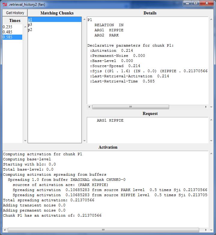
87 Retrievals Pressing this button opens a new Retrievals window for the current data source and any number of those windows may be open. Here is a display of the window without any data shown (how it will always appear upon opening): 87

88 To display the recorded data you need to press the Get History button in the upper-left corner of the window. Here is what the window shows after pressing Get History for a run of the fan model from unit 5 of the tutorial for the sentence the hippie is in the park using the person as the retrieval cue: The left column displays all the times at which a retrieval request was made. Selecting one of those times will cause the Matching Chunks section of the window to list all of the 88

89 chunks that were in declarative memory and matched the request at that time. The item at the top of the list is the one which was retrieved, or will be the keyword :retrieval-failure if no chunk was retrieved. The rest of the chunks in the list are in no particular order. The Request section of the window will display the request which was made at that time. Selecting one of the chunks from the Matching Chunks list will result in the Details section being filed with a printing of the chunk along with the parameter values for that chunk at the time of the retrieval request. The Activation section of the display will show the detailed activation trace of how that chunk s activation was computed at that time. Here is the tool after selecting the second time and the first chunk on the resulting list, p1: 89

90 90

91 Buffers Pressing this button opens a new Buffers window for the current data source and any number of those windows may be open. Here is a display of the window without any data shown (how it will always appear upon opening): To display the data you need to press the Get History button in the upper-left corner of the window. Here is what the window shows after pressing Get History following a run of the fan model from unit 5 of the tutorial for the sentence the hippie is in the park with the default set of buffers for the model being recorded: 91

92 The left column displays all the times at which a change occurred in some buffer, where a change is any of: the buffer clearing, a chunk being placed into the buffer, the chunk in the buffer being modified, or a change in one of the buffer queries of state free, state busy or state error. The middle column shows the names of all the buffers for which data was recorded. Selecting a time and one of the buffers will result in the Details section being filed with the results from calling buffer-status and buffer-chunk for that buffer at the time specified. Here is the tool after selecting the 0.25 seconds time and the imaginal buffer: 92

93 One thing to note is that the information shown for the buffer is how it was reported at the end of the time selected. There may have been multiple changes occurring in the buffer during that time step (multiple concurrent events), but only the final state is recorded. Audicon Pressing this button opens a new Audicon window for the current data source and any number of those windows may be open. Here is a display of the window without any data shown (how it will always appear upon opening): 93

94 To show the data you need to press the Get History button in the upper-left corner of the window. Here is what the window shows after pressing Get History following a run of the sperling model from unit 3 of the tutorial with a delay of.15 seconds: The left column displays all the times at which a change in the audicon information occurred. Selecting a time will result in the Audicon section being filed with the output from having called print-audicon at the time specified. Here is the display after selecting the seconds time: 94

95 Visicon Pressing this button opens a new Visicon window for the current data source and any number of those windows may be open. Here is a display of the window without any data shown (how it will always appear upon opening): To show the data you need to press the Get History button in the upper-left corner of the window. Here is what the window shows after pressing Get History following a run 95

96 of the sperling model from unit 3 of the tutorial with a delay of.15 seconds: The left column displays all the times at which a change in the visicon information occurred. Selecting a time will result in the Visicon section being filed with the output from having called print-visicon at the time specified. Here is the display after selecting the seconds time: 96

97 BOLD tools There are three tools which can provide graphic representations of the BOLD (Blood Oxygen Level Dependent) response prediction data which a model generates. A full description of how that is computed is beyond the scope of this document, but a very brief description will be given here before describing the tools (more details can be found in the ACT-R Reference Manual). For each buffer in ACT-R the pattern of use, as shown in the graphic traces, can be recorded. That recorded pattern of use over a run can then be considered as a metabolic demand on the brain which can be combined with a hemodynamic response function to create a prediction of a BOLD response. Past research has lead to associating each of the buffers in ACT-R with a particular region of the brain. Thus, the patterns of use of the buffers lead to predictions for a BOLD response seen across various areas of the brain. BOLD Graphs The BOLD Graphs button will open up a new BOLD Graphs window for the current data source and any number of those windows may be open at a time. Here is a display of the window without any data shown (how it will always appear upon opening): 97

98 The column on the left side lists all the buffers in the model. Selecting a buffer from the list will result in a graph being drawn in the pane on the right of the window showing the data returned by the ACT-R predict-bold-response command for that buffer, scaled into the range Here is the graph for the retrieval buffer after running the paired associate learning model from unit 4 of the tutorial for two items five trials each by evaluating (paired-task 2 5): 98

99 The + and - buttons at the top can be used to zoom in or out on the graph and here is that same graph after zooming out to show more of the data: 99

100 The Start and Stop boxes can be used to restrict the display to a particular segment of the run. Each box can have a time in seconds entered in it. If the Start box is empty then the data is started at time 0s, and if the Stop box is empty then the end time is the stopping time of the model run. After adjusting the Start and Stop values you must hit the Redisplay button to have the graph redrawn. Here is that same trace restricted to the time between 10 and 20 seconds in the run at a different zoom level: 100

101 Note that the data may not always fit into exactly the times specified. That is because the data is generated based on an interval specified in the model with the :bold-inc parameter which defaults to 2 seconds, and adjusting the Start and Stop times does not change the interval used. It always starts incrementing from time 0 and plots the data based on the middle of each the interval. It is also possible to select more than one buffer in the column on the left. Each selected buffer will be drawn in the current display. The selection color of the buffer corresponds to the color of that buffer s data in the graph. Here is the data from the retrieval and visual buffers both shown in the same display for that task: 101

102 If the Scale across regions box is unchecked then for each buffer the BOLD data is scaled to the range of for display based on the maximum value for that buffer. If the Scale across regions box is checked, then the data for all buffers is scaled to the range based on the maximum value among all the buffers. This allows one to see the effects more clearly for a given buffer or to compare the results from different regions when desired. Here is the same data with the Scale across regions box checked: 102

103 BOLD 2D brain The BOLD 2D brain button will open a new BOLD Brain window for the current data source and any number of those windows may be open at a time. Here is what the window looks like when first opened: 103

104 The buffers for which a brain association is defined are displayed on the left in the color which will be used to draw them in the images and in the order in which they are drawn in the images i.e. the manual buffer is drawn in the top slices and the visual buffer in the lower ones. If the Show box borders button is selected then a colored box will be displayed for each buffer whether or not there is any activity. This can be used to see where the regions are in the absence of any activity and looks like this without any other data displayed: 104

105 The slider along the bottom allows one to select the specific scan from the run for which the data should be displayed. The scans occur based on the value of the :bold-inc parameter, with a scan occurring every :bold-inc seconds. On each scan the brightness of the corresponding boxes indicates the BOLD activity in that buffer. Each buffer has its BOLD data scaled from individually and that is used as a brightness value in displaying the color. Thus, if there is no activity, a value of 0, then the box will be black and if there is a lot of activity, a value near 1.0, then the box will be brightly colored. Here is an image from the paired associate model as run for the graphing data at scans

106 showing activity in several buffers increasing at the start of the task: 106

107 107

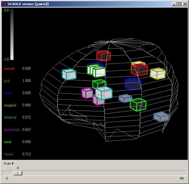
108 BOLD 3D brain The BOLD 3D brain button will open a new BOLD 3D Brain window for the current data source and any number of those windows may be open at a time. These windows show the same information as the 2D viewer described above, except that instead of the using images from a reference brain the boxes are drawn in a very crude three-dimensional wireframe brain model. Here is what the window looks like by default: 108

109 The buffers for which a brain association is defined are displayed on the left in the color which is used to draw the outline of the region s box in the image. The default view is top-down with the front of the brain to the left, but the brain can be rotated and moved by clicking on it and moving the mouse. If the left mouse button is clicked and held moving the mouse will rotate the brain around its center point. If the right mouse button is clicked and held moving the mouse up and down will zoom in and out on the image, and if the middle mouse button is clicked and held moving the mouse will move the brain around in the window without rotating it. Here is a view of the image after it has been moved and rotated: 109

110 The slider along the bottom allows one to select the specific scan from the run for which the data should be displayed in the same way that it does for the 2D viewer. On each scan the boxes for each buffer will be filled with a gray-scale color which indicates the BOLD activity in that buffer at that time. There is a reference scale of the gradient shown in the upper left of the window. The box outlines will always be drawn with the brightly colored edges. Each buffer has its BOLD data scaled from individually and that is used as a brightness value in displaying the color and that number is also shown on the left of the window after the buffer name. Here is an image from the paired associate model as run for the graphing data on scan 4 showing activity in several buffers: 110

111 111

112 Miscellaneous The Miscellaneous section contains the controls which are not involved with the actually modeling and thus do not belong to one of the other sections. The only control in the current Environment is the Options button which allows the user to specify some settings for how the Environment should operate. Options Pressing the Options button will bring up the Options window if it is not already open or bring it to the front if it is open because there can only be one such window open at a time. Here is what the Options window looks like: It has several options which can be enabled or disabled by checking or unchecking them. When the window is opened the current setting of the options will be shown in the selections. Some of the options are only meaningful when using the editor with the standalone version of the Environment, but they will all be described below for completeness. First, the buttons at the bottom of the window will be described, and then each of the options themselves. 112

113 Save Pressing the Save button will apply the current selections to the Environment as well as save them to a file so that the next time the Environment is started those settings will be used instead of the defaults. It will also close the Options window after saving the settings. Apply Pressing the Apply button will apply the current selections to the Environment to change how it operates. It does not save those setting for future use nor does it close the window. Cancel Pressing the Cancel button will close the window without applying or saving any of the changes which have been made to the options since the last save or apply occurred. Revert Pressing the Revert button will return all of the options to the values which they had when last applied or saved, undoing any changes that have been made. It does not close the window, nor does it save or apply the values. Use an Environment window for the Experiment display This option is only meaningful if ACT-R is running in a Lisp which has GUI tools available and which also has the appropriate support in the ACT-R graphics interface. At this time those Lisps would be ACL w/ide, LispWorks, and CCL. If ACT-R is running in any other Lisp, then the selection of this box is ignored. The default for this option is selected (enabled) which means that when the Environment is connected to ACT-R any experiment window opened with the ACT-R open-exp-window command which is visible will be displayed in a window opened by the Environment in 113

114 Tcl/Tk instead of with the Lisp s native GUI tools. If the option is disabled then the Lisp s native GUI tools will be used to display visible windows opened with the openexp-window command. Compile definitions when model opened or reloaded This option controls how models are loaded or reloaded through the Environment. If the box is unchecked (the default) then files which are loaded or opened with the Load Model or Open Model buttons (note that Open model is only available by default with the standalone version) are loaded directly with the Lisp command load, and when the Reload button is pressed the ACT-R reload command is called with no parameters. If the option is enabled then when a file is loaded or opened the file is first compiled with the Lisp command compile-file and then that compiled file is loaded with the load command. When the Reload button is pressed with this option enabled the value of t is provided as the optional parameter to the reload command which will cause it to also compile the file before loading. One thing to note about having the parameter enabled is that if you directly load a compiled file then the Reload button will not work for that file because it will not be able to compile the already compiled file and it will print this warning instead: # Warning: To use the compile option the pathname must have type lisp. # Automatically save an open model when reload pressed This option only affects the operation of the Environment when using the Open model button available with the standalone version (or enabled by the user as described in the Extending or Changing the Environment section). If this option is enabled, which is the default, then any changes made to the currently open model file will be saved before the reload command is called in response to pressing the Reload button. If this option is not checked then the changes will not be saved by the Environment prior to the reload command being called and thus the previously saved version will be loaded. 114

115 Show the ACT-R copyrights screen This option controls whether or not the window showing the ACT-R copyright information is displayed every time the Environment is started. If it is enabled then the window will be displayed and if it is disabled then it will not be displayed. Save a backup every time This option only affects the operation of the Environment when using the Open Model: button. If this option is enabled, then whenever the model file is saved (including the automatic saving upon reload if enabled) a backup copy of the existing file is made first. The backup copy will have the same name as the original file with an increasing number added to the end of the file s extension. It will be written to the same directory as the original file. Thus, if the count.lisp file were opened and then reloaded a file named count.lisp-0 would be created in the same directory as the original count.lisp file and would be a copy of the file count.lisp before any current changes are saved into it. If it were reloaded again then a file named count.lisp-1 would be created, and so on. These backup files are intended only as protection against a crash of the system or other error which may cause the loss of the file being worked on. The original file will always be the most recently saved version of the model and you should not open or load the backup files directly unless absolutely needed. After the Environment has been successfully closed you should feel free to delete any and all of the backup files. If the system does crash or for some other reason you would like to use one of the backup files you should first rename it to something meaningful if you plan to open it in the Environment because otherwise it will also have backups made of it which would then look something like count.lisp-1-0 and that can become confusing very quickly. Allow the environment to work with multiple models This option controls whether the Environment assumes there will only ever be one model defined at a time, or if it will provide separate tools for multiple simultaneously defined models. The default setting is off. In that case if more than one model is defined this 115

116 warning will be displayed: If the setting is enabled, then it will show this dialog when that change is made: To change the Environment safely from single model mode to multiple model mode requires stopping and starting the connection to Lisp. Thus, when making that change the Save button should always be used to make the change because the Apply button s settings do not persist across a stopping and starting of the Environment. Close inspector windows for deleted models when multiple models are defined This option only matters if the Allow the environment to work with multiple models option is enabled. If that is enabled then this controls what happens to the inspector windows for models which are no longer defined. If the option is set then when a model is deleted the inspector windows for that model will automatically be closed in the Environment. If it is not set then the windows for deleted models will remain open, but will no longer function correctly and trying to use them may result in warnings in the Lisp running ACT-R. Show warning when opening stepper if :v is nil in all models This option controls whether or not a warning is displayed when the stepper is opened and all of the current models have the :v parameter set to nil. The stepper requires trace 116

117 output to be able to step, thus if :v is nil in all models the stepper will not work. Note however that the value of :v could be changed between when the stepper is opened and when the model is run. Thus, just because the trace is turned off in all models at the time the stepper is opened does not mean that will necessarily be the case when the models are run. The default setting is on. 117

118 Window Positions and Sizes When the Environment is closed it will save all of the settings for the window sizes and positions that were used while it was running. The next time that the Environment is run it will then use those same sizes and positions for all of the windows. This is generally desirable, but can lead to problems if one uses the same machine with different displays or monitors which have different resolutions which could result in windows or tools no longer being within the bounds of the current display. To accommodate that there is a test performed when the Environment first starts to check whether or not the same screen space is available by testing the current height and width as well as the maximum window size as reported by the system. If those differ, then it will display this dialog before starting with the option of restoring everything to the default size and location instead of using the saved values: If the Yes option is chosen then the default window positions will be used instead of those in the saved configuration. If for some reason the Environment doesn t detect that your screen has changed or you are having some other problems whereby the tools are no longer available because they are opening in windows outside of the screen then you can manually remove the file with the saved settings in it and force things into their default positions the next time the Environment is started. The settings are saved in the Environment s GUI/init directory in the file named 10-userguisettings.tcl. If you delete that file then the next time the Environment starts all of the windows will revert to their default sizes and positions. 118

119 Extending or Changing the Environment It is possible to add new tools or capabilities to the Environment. Like the ACT-R loader, when the Environment starts it will automatically load source files located in some of its directories. Thus, putting new files into those directories will cause that additional code to be loaded and become a part of the Environment. Changes to the operations can also be made on the Lisp side of the Environment (which may affect how things are displayed or otherwise generated for display on the Tcl/Tk side) by placing files into the ACT-R directories that get loaded automatically. When the Environment starts it first loads all of the.tcl files in the GUI/init directory. Then, it opens the Control Panel window and loads all of the.tcl files located in the GUI/dialogs directory. The files are loaded in ascending order based on their file names. It is also possible to remove tools that you don t need, if you don t want them included in the Environment, by deleting those files from the GUI/dialogs directory. Each of the tools in the Environment is generally implemented in a separate file located in the dialogs directory and the names of the files indicate the tool that they implement, for example 38visicon.tcl implements the Visicon button. Deleting that file will remove the Visicon button from the Environment. The numbers on the fronts of the names are used to ensure that they are loaded and created in a specific order. Most of the tools are independent and can be deleted without affecting the others, but there are a couple of exceptions. First, the 00-copyrights.tcl file should not be deleted because it also controls the initial connection between ACT-R and the Environment. To eliminate the copyright window you should instead disable the Options setting which controls it. Also, the standalone version of the Environment s buttons for closing and saving model files depend on operations defined in the open model tool. Thus, if the open button is removed the save and close buttons should also be removed. There are some additional controls or modifications for the Environment included with the ACT-R extras which can be used and are described in the sections below. There are also some disabled buttons (like the Open button mentioned above) included in the 119

120 GUI/dialogs directory. They were disabled by changing the extension on the file name from.tcl to.tcx. Returning that to.tcl will enable that button. 120

121 Available Environment Extras In the extras directory of ACT-R there are two additional tools which can be added to the Environment, and the examples directory contains an example of extending the virtual window device for a model and having the Environment generated visible windows display the new item. Each of those will be described below along with how to add it to the Environment. Sorted Items This extra capability will change the operation of all the list boxes of items in the inspector windows so that their values are sorted alphabetically instead of the default ordering returned by ACT-R. This will affect the listings in the Declarative, Procedural, Buffer, and Buffer Status tools. There are two ways to make this extension available. It can be enabled at anytime by using the require-extra command in ACT-R specifying "environment-sorter" as the extra: (require-extra "environment-sorter") Alternatively, the file called sort-environment-lists.lisp in the extras/environment-sorter directory can be explicitly loaded into ACT-R. To have that file loaded every time one loads ACT-R, it can be moved to the user-loads directory of the ACT-R source code. DM Tree Viewer In the extras/chunk-tree-viewer directory are several files which describe and implement a declarative viewer with an alternative display of chunks. The representation was developed by Andrea Heiberg, Jack Harris, and Jerry Ball working at the Air Force Research Laboratory and is described in detail in the HeibergHarrisBall.pdf file found in that directory. The tool for the Environment is a slight modification to their representation and is described in detail below. To use the tool the chunk-tree.lisp file should be placed into the ACT-R other-files 121

122 directory and the 35a-declarative-tree.tcl file should be placed into the Environment s GUI/dialogs directory. Doing so will add a new button called DM Tree viewer to the Current Data section of the Control Panel. Pressing that button will open a new declarative_tree window for the current model and any number of those windows may be open at a time. Here is what the window will look like after running the fan model from the tutorial unit 5 (note that the sorted items addition described above is also loaded here): Like the normal declarative viewer the list on the left shows the names of all the chunks in the model s declarative memory and the filter at the top can be used to restrict that list to chunks which have a particular set of slots. The difference in the display of the selection along with the additional controls available for this dialog will be described below. Selecting one of the chunks from the list will result in an image being generated to show the contents of that chunk. The chunk name will be displayed at the top of the window in 122

123 light green and then for each slot a blue line will be drawn below that name with the name of the slot written in blue italic text at the end of the line. Below the slot name the contents of the slot will be displayed. If the content is not a chunk then it will be displayed in black with nothing below it. If the content is a chunk, then it will be displayed in one of three ways. If it is a chunk which is not in the model s declarative memory and which doesn t occur further up in the current branch of the tree then it will be displayed in dark green text with its slot contents displayed recursively below it. If it is a chunk which does occur in the model s declarative memory and which doesn t occur further up in the current branch of the tree then it will be displayed in light green text and its slots will be recursively displayed below it. If it is a chunk which has already been displayed in the current branch of the tree (a circular reference) then it will be displayed in red text and its slots will not be displayed. Here is the display for the chunk0-0 chunk after the model has done a trial for the giant is in the park : It shows the contents of the arg1 and arg2 slots as the chunks hippie and park and each of those chunks has a word slot which contains the string representation of that word. 123

124 For demonstration purposes, these commands have been executed to define some additional chunks for the model and to add a new chunk to the model s declarative memory: (chunk-type demo-type slot1 slot2) (define-chunks (simple isa chunk) (circular isa demo-type slot1 simple slot2 circular)) (add-dm (demo-chunk isa demo-type slot1 circular slot2 simple)) Thus, the demo-chunk is in the model s declarative memory while the simple and circular chunks are not, and the chunk named circular has a slot with a circular reference to itself. Here is the display showing the chunk named demo-chunk being drawn: 124

125 Any of the light green chunks in the display (the chunks which are in the model s declarative memory) can be clicked on to open the Environment s declarative tool with that chunk selected to see the parameters and text representation of that chunk. Pressing the Save button at the top right of the declarative tree viewer window will allow you to save an image of the chunk as an Encapsulated PostScript file. A file creation dialog will be opened and the image will be saved into the file which you provide. Extending the visible virtual windows In the examples/creating-a-new-virtual-item directory of ACT-R are some files which demonstrate how to extend the virtual windows which can be used for an ACT-R device. The example extension creates an image feature for models and the example code contains an extension for the Environment which will draw a.gif format file in the visible virtual window for that item. See the details in the readme.txt file of the example for more details. 125

126 Standalone Environment Tools The standalone version of the Environment includes some additional buttons in the model section of the Control Panel: These buttons provide access to a very basic text editor which can be used to edit or create models. Open Model: The Open Model: button will either create a new text file or open an existing file depending on the setting of the option menu to its right. If the option menu says Existing then a dialog will open for you to select a file to open and edit. If the option menu says New then a dialog will open asking you for the name and location to save the new file. To change the option menu you can press it to bring up the options which will look like this: The one with the checkmark is the currently selected option and clicking the other will make it the current option. In addition to opening the file for editing, it will also be loaded as if it had been chosen using the Load Model button. There can only be one model opened for editing in the 126

127 Environment at any time. If you try to open a second one it will display a warning dialog indicating that you must close the currently open model first: You can close an open model using the Close Model button on the Control Panel or by just closing the window in which it is being edited. Save Model The Save Model button will save the contents of the currently opened model file. If there is no model currently opened for editing, then this button has no effect other than to display a dialog indicating that there is not an open model: If the Save a backup every time option is enabled, then before the file is saved a backup copy of the previous file will be made. Close Model The Close Model button will save the contents of the currently opened model file and close the window in which it is being edited. 127