MAT 110 WORKSHOP. Updated Fall 2018

Size: px

Start display at page:

Download "MAT 110 WORKSHOP. Updated Fall 2018"

Edith Hines
5 years ago
Views:

1 MAT 110 WORKSHOP Updated Fall 2018

2 UNIT 3: STATISTICS Introduction

3 Choosing a Sample Simple Random Sample: a set of individuals from the population chosen in a way that every individual has an equal chance to be chosen. Stratified Samples: A series of SRS s performed on subgroups (strata) of a given population Systematic Sampling: Taking every kth member of the population. The first individual selected corresponds to a random number between 1 and k. Cluster Sampling: Taking all the individuals within a randomly selected collection or group of individuals.

4 Definitions Mean: The average in a set of data. Median: The middle number in an ordered list. If there are two middles, the median is the average of those two. Mode: The number(s) that appears the most frequently in a data set. Range: The difference between the largest and smallest values. Standard Deviation: An average measure of how far each data point is from the mean. Normal Distribution: A very common distribution that describes many real life values. The symmetric Bell curve. Z-Score: The number of standard deviations a value is from the mean. Confidence Interval: A range that is 'likely' to contain the actual mean of a data set. Usually associated with a margin of error. Margin of error: The likelihood that a confidence interval does NOT contain the mean of a data set.

5 Example Find the mean, median, and mode for the following data: 12, 21, 11, 6, 24, 11, 23, 9, 15, 11

6 Example 6, 9, 11, 11, 11, 12, 15, 21, 23, 24 Mean = 143 because = 143 and there are 10 numbers Median = 11.5 because 11 and 12 are the middle numbers when placed smallest to largest, so we take the average of the two. Mode = 11 because it appears 3 times while all the other numbers only appear once.

7 Calculate the five number summary and create a Box and Whiskers Plot for the following data: 12, 21, 11, 6, 24, 11, 23, 9, 15, 11

8 Minimum=6 6, 9, 11, 11, 11, 12, 15, 21, 23, 24 Lower Quartile Q 1 = 11 because it is in the middle of the numbers below the median. Median = 11.5 because 11 and 12 are the middle numbers when placed smallest to largest, so we take the average of the two. Upper Quartile Q 3 = 21 because it is in the middle of the numbers above the median. Maximum=24

9 Stem and Leaf Display Example: The following are the number of home runs hit by the home run champions in the National League for the years 1975 to 1989 and for 1993 to : 38, 38, 52, 40, 48, 48, 31, 37, 40, 36, 37, 37, 49, 39, : 46, 43, 40, 47, 49, 70, 65, 50, 73, 49, 47, 48, 51, 58, 50 Compare these home run records using a stem-andleaf display. (continued on next slide)

10 Stem and Leaf Display Solution: In constructing a stem-and- leaf display, we view each number as having two parts. The left digit is considered the stem and the right digit the leaf. For example, 38 has a stem of 3 and a leaf of to to 2007 (continued on next slide)

11 Stem and Leaf Display We can compare these data by placing these two displays side by side as shown below. Some call this display a back-to-back stem-and-leaf display. It is clear that the home run champions hit significantly more home runs from 1993 to 2007 than from 1975 to 1989.

12 The Five Number Summary Example: Consider the list: 42, 43, 46, 51, 51, 51, 52, 54, 55, 55, 56, 56, 60, 61, 61, 64, 69. Find the following for this data set: a) the lower and upper halves b) the first and third quartiles c) the five-number summary (continued on next slide)

13 The Five Number Summary Solution: (a): Finding the median, we can identify the lower and upper halves. (b): The median of the lower half is The median of the upper half is (continued on next slide)

14 The Five Number Summary (c): The five number summary is We represent the five-number summary by a graph called a box-and-whisker plot. (continued on next slide)

15 Example Find the five-number summary for the following 10 values: 40, 37, 32, 28, 27, 24, 22, 34, 19, 36 Find the minimum: Find Q1: Find the median: Find Q3: Find the maximum:

16 Example 19,22,24,27,28,32,34,36,37,40 Minimum: 19 because that is the smallest number Q 1 : 24 because it is in the middle of the minimum and median Median: 30 because it is in the very middle of the numbers = 30 Q 3 : 36 because it is in the middle of the median and the maximum Maximum: 40 because it is the largest number

17 Histograms A researcher surveyed 90 patients at a certain hospital. The histogram below gives the length of time patients waited to see a doctor at the hospital. The bins in minutes are 5-9.9, ,, etc and the vertical axis represents the number of patients. a) Use the histogram to sketch a box and whiskers plot.

18 Histograms A researcher surveyed 90 patients at a certain hospital. The histogram below gives the length of time patients waited to see a doctor at the hospital. The bins in minutes are 5-9.9, ,, etc and the vertical axis represents the number of patients. a) Use the histogram to sketch a box and whiskers plot. Min: 5-10 Q 1 : Median: Q 3 : Max: 40-45

19 Histograms A researcher surveyed 90 patients at a certain hospital. The histogram below gives the length of time patients waited to see a doctor at the hospital. The bins in minutes are 5-9.9, ,, etc and the vertical axis represents the number of patients. a) Use the histogram to sketch a box and whiskers plot. Min: 5-10 Q 1 : Median: Q 3 : Max: 40-45

20 Histograms A researcher surveyed 90 patients at a certain hospital. The histogram below gives the length of time patients waited to see a doctor at the hospital. The bins in minutes are 5-9.9, ,, etc and the vertical axis represents the number of patients. a) What percent of patients waited more than 20 minutes to see a doctor?

Histograms A researcher surveyed 90 patients at a certain hospital. The histogram below gives the length of time patients waited to see a doctor at the hospital.

21 Histograms A researcher surveyed 90 patients at a certain hospital. The histogram below gives the length of time patients waited to see a doctor at the hospital. The bins in minutes are 5-9.9, ,, etc and the vertical axis represents the number of patients. a) What percent of patients waited more than 20 minutes to see a doctor? = 0.4 or 40%

22 The Range of a Data Set

23 Standard Deviation

24 Standard Deviation Example: A company has hired six interns. After 4 months, their work records show the following number of work days missed for each worker: 0, 2, 1, 4, 2, 3 Find the standard deviation of this data set. Solution: Mean: (continued on next slide)

25 Standard Deviation We calculate the squares of the deviations of the data values from the mean. Standard Deviation:

26 The Normal Distribution The normal distribution describes many real-life data sets. The histogram shown gives an idea of the shape of a normal distribution.

27 The Normal Distribution

28 The Normal Distribution We represent the mean by μ and the standard deviation by σ.

29 The Normal Distribution Example: Suppose that the distribution of scores of 1,000 students who take a standardized intelligence test is a normal distribution. If the distribution s mean is μ = 450 and its standard deviation is σ = 25, a. How many scores do we expect to fall between 425 and 475? b. How many scores do we expect to fall above 500? (continued on next slide)

30 The Normal Distribution Solution (a): 425 and 475 are each 1 standard deviation from the mean. Approximately 68% of the scores lie within 1 standard deviation of the mean. We expect about ,000 = 680 scores are in the range 425 to 475. (continued on next slide)

31 The Normal Distribution Solution (b): We know 5% of the scores lie more than 2 standard deviations above or below the mean, so we expect to have = of the scores to be above 500. Multiplying by 1,000, we can expect that ,000 = 25 scores to be above 500.

32 Quartile Problem The scores of students on an exam are normally distributed with a mean of 516 and a standard deviation of 36. A) What is the first quartile score for this exam? B) What is the third quartile score for this exam?

33 Quartile Problem The Quartiles have 25% of the data on either side so we can use the area to find the Z-Score which is ± A) x = so the first quartile is at B) x = so the third quartile is at

34 z-scores The standard normal distribution has a mean of 0 and a standard deviation of 1. There are tables (see next slide) that give the area under this curve between the mean and a number called a z-score. A z-score represents the number of standard deviations a data value is from the mean. For example, for a normal distribution with mean 450 and standard deviation 25, the value 500 is 2 standard deviations above the mean; that is, the value 500 corresponds to a z-score of 2.

35 z-scores Below is a portion of a table that gives the area under the standard normal curve between the mean and a z-score.

36 z-scores Example: Use a table to find the percentage of the data (area under the curve) that lie in the following regions for a standard normal distribution: a. Between z = 0 and z = 1.3 b. Between z = 1.5 and z = 2.1 c. Between z = 0 and z = 1.83 (continued on next slide)

z-scores Solution (a): The area under the curve between z = 0 and z = 1.3 is shown. Using a table we find this area for the z-score 1.30.

37 z-scores Solution (a): The area under the curve between z = 0 and z = 1.3 is shown. Using a table we find this area for the z-score We find that A is when z = We expect 40.3%, of the data to fall between 0 and 1.3 standard deviations above the mean. (continued on next slide)

38 z-scores Solution (b): The area under the curve between z = 1.5 and z = 2.1 is shown. We first find the area from z = 0 to z = 2.1 and then subtract the area from z = 0 to z = 1.5. Using a table we get A = when z = 2.1, and A = when z = 1.5. The area is = or 4.9% (continued on next slide)

39 z-scores Solution (c): Due to the symmetry of the normal distribution, the area between z = 0 and z = 1.83 is the same as the area between z = 0 and z = Using a table, we see that A = when z = Therefore, 46.6% of the data values lie between 0 and 1.83.

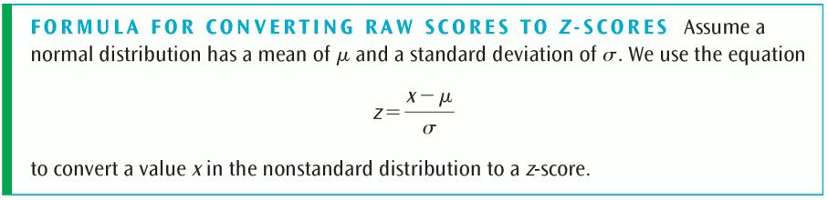
40 Converting Raw Scores to z-scores

41 Converting Raw Scores to z-scores Example: Suppose the mean of a normal distribution is 20 and its standard deviation is 3. a) Find the z-score corresponding to the raw score 25. b) Find the z-score corresponding to the raw score 16. (continued on next slide)

42 Converting Raw Scores to z-scores Solution (a): We have We compute (continued on next slide)

43 Converting Raw Scores to z-scores Solution (b): We have We compute

44 Applications Example: Suppose you take a standardized test. Assume that the distribution of scores is normal and you received a score of 72 on the test, which had a mean of μ = 65 and a standard deviation of σ = 4. What percentage of those who took this test had a score below yours? Solution: We first find the z-score that corresponds to 72. (continued on next slide)

45 Applications Using a table, we have that A = when z = The normal curve is symmetric, so another 50% of the scores fall below the mean. So, there are 50% + 46% = 96% of the scores below 72. (continued on next slide)

46 Applications Example: Consider the following information: 1911: Ty Cobb hit.420. Mean average was.266 with standard deviation : Ted Williams hit.406. Mean average was.267 with standard deviation : George Brett hit.390. Mean average was.261 with standard deviation Assuming normal distributions, use z-scores to determine which of the three batters was ranked the highest in relationship to his contemporaries. (continued on next slide)

47 Applications Solution: Ty Cobb s average of.420 corresponded to a z- score of Ted Williams s average of.406 corresponded to a z- score of George Brett s average of.390 corresponded to a z- score of Compared with his contemporaries, Ted Williams ranks as the best hitter.

48 Applications Example: A manufacturer plans to offer a warranty on an electronic device. Quality control engineers found that the device has a mean time to failure of 3,000 hours with a standard deviation of 500 hours. Assume that the typical purchaser will use the device for 4 hours per day. If the manufacturer does not want more than 5% to be returned as defective within the warranty period, how long should the warranty period be to guarantee this? (continued on next slide)

49 Applications Solution: We need to find a z-score such that at least 95% of the area is beyond this point. This score is to the left of the mean and is negative. By symmetry we find the z-score such that 95% of the area is below this score. (continued on next slide)

50 Applications 50% of the entire area lies below the mean, so our problem reduces to finding a z-score greater than 0 such that 45% of the area lies between the mean and that z-score. If A = 0.450, the corresponding z- score is % of the area underneath the standard normal curve falls below z = By symmetry, 95% of the values lie above Since, we obtain (continued on next slide)

51 Applications Solving the equation for x, we get Owners use the device about 4 hours per day, so we divide 2,180 by 4 to get 545 days. This is approximately 18 months if we use 31 days per month. The warranty should be for roughly 18 months.

52 Right and Left Z-Score Find the z-score such that: A) The area under the standard normal curve to its left is B) The area under the standard normal curve to its left is C) The area under the standard normal curve to its right is D) The area under the standard normal curve to its right is

53 Right and Left Z-Score A) = look this up in the table to get 0.04 B) = look this up in the table to get 0.91 C) =.2121 look this up in the table to get 0.56 D) =.1427 look this up in the table to get 0.36

54 Practice Problem Length of skateboards in a skateshop are normally distributed with a mean of 30.9 in and a standard deviation of 1 in. The figure below shows the distribution of the length of skateboards in a skateshop. Calculate the shaded area under the curve. Express your answer in decimal form with at least two decimal place accuracy.

55 Practice Problem There is an area of.475 on the right side of the curve but we must use the Z-Score formula to find the area on the left side. z = = -.67 The area at Z-Score of -.67 is So the total area is =.7236

56 ҧ Confidence Intervals A level C confidence interval is a range that is C% likely to contain the population mean of a set of data based on a sample mean (a 95% confidence interval based on sample data would be 95% likely to contain the population mean that the sample came from). The formula for the lower and upper bounds of a confidence interval is: x ± z σ n Where the term on the left is the sample mean, and the term on the right is referred to as the margin of error. To find the critical value, z for a level C confidence interal: 1. Write C as a decimal and find C 2 This is the area between z=0 and z on the standard normal curve. 2. Find the z-score in your table with the area closest to C between it and z=0. This 2 is your z.

57 Confidence Intervals Example: Suppose that the distribution of scores of 100 students who take a standardized intelligence test is a normal distribution. If the distribution s sample mean is 90 and its standard deviation is 10, what is a 95% confidence interval for the population mean? Here, the critical value z is.95 2 =.475 Locating this area in a z-score table will yield that z = The left end of the interval is: = The right end of the interval is: = So the 95% confidence interval is (88.04, 91.96), OR we are 95% confident the population mean is between and

58 Normal Distribution Exercises Suppose 200 students took a test, and their scores were approximately normally distributed. The mean of the test scores was μ = 82 and the standard deviation was σ = 9. How many students got at least a 73? How many students got more than 95? What would a 95% confidence interval for this population be?

59 Normal Distribution Solutions n = 200, μ = 82, σ = 9 (a) How many students got at least a 73? (b) More than 95? (c) What would a 95% confidence interval for this population be? (a).84 or 84% (168 students) (b).075 or 7.5% (15 students) (c)(80.75, 83.25)

60 Margin of Error Scores on a standardized exam are known to follow a normal distribution. A researcher estimates the mean score on a standardized exam to be between 69 and 76 with a 98% confidence interval. What is the margin of error?

61 ҧ ҧ Margin of Error Scores on a standardized exam are known to follow a normal distribution. A researcher estimates the mean score on a standardized exam to be between 69 and 76 with a 98% confidence interval. What is the margin of error? Remember the confidence interval is found by adding or subtracting the margin of error to/from the mean. So 69 + Error = x and 76 Error = x You can also say = Error 2 So the Margin of Error is 3.5.

62 Confidence Intervals and Margin of Error The heights of Christmas trees are known to follow a normal distribution with a standard deviation of 8 inches. A researcher wants to estimate the mean height of all Christmas trees. If she wants to estimate this with an 81% confidence interval, what size sample size should she use to estimate the mean tree height to within ±5 inches.

63 Confidence Intervals and Margin of Error The heights of Christmas trees are known to follow a normal distribution with a standard deviation of 8 inches. A researcher wants to estimate the mean height of all Christmas trees. If she wants to estimate this with an 81% confidence interval, what size sample size should she use to estimate the mean tree height to within ±5 inches. If we want the mean tree height to be within 5 inches, then the margin of error is 5. We will use z σ n = Error To find z use =.405 and see that the closest z-score would be So 5 = n Then n = 4.39, but we cant have.39 of a tree We need a sample of 5 trees.

64 Thank you for coming!

The first few questions on this worksheet will deal with measures of central tendency. These data types tell us where the center of the data set lies.

The first few questions on this worksheet will deal with measures of central tendency. These data types tell us where the center of the data set lies. Instructions: You are given the following data below these instructions. Your client (Courtney) wants you to statistically analyze the data to help her reach conclusions about how well she is teaching.