AnalyzeLoad User s Manual

Size: px

Start display at page:

Download "AnalyzeLoad User s Manual"

Natalie Dalton
5 years ago
Views:

1 Box Elder Innovations, LLC Bear River City, Utah AnalyzeLoad User s Manual 1.0 Introduction AnalyzeLoad is a set of computer programs that have at their core physics-based interior and exterior ballistics models developed by Box Elder Innovations, LLC. The intent of these programs is to provide the shooting community with inexpensive tools for generating computational data to aid in the development and understanding of safe loads for small arms ammunition, for failure investigations, and for computing the influence of unknown conditions on cartridge performance. AnalyzeLoad comes in three versions, AnalyzeLoad(1.x), AnalyzeLoad(2.x) and AnalyzeLoad(3.x). AnalyzeLoad(1.x) has the capabilities listed under 1) and 4) below, AnalyzeLoad(2.x) has the capabilities listed under 1) to 3), below, and AnalyzeLoad(3.x) has all the capabilities listed below. These capabilities are: 1) Forward calculation interior ballistics module for computing muzzle velocity, pressure vs. time curves, pressure vs. bullet position (x) in the barrel, velocity vs. x, and mass of propellant vs. x. AnalyzeLoad(1.0) and AnalyzeLoad(2.0). 2) Sensitivity analysis module for computing the forward interior ballistics calculation output, P(t), sensitivity to the primary gun and cartridge model input properties. AnalyzeLoad(2.0) only. 3) Inverse interior ballistics calculation module for computing the i) bullet/barrel friction constant given measured values for muzzle velocity, bullet weight, barrel length, and powder weight for a selected cartridge and powder type, or ii) propellant burn rate constants given values for muzzle velocity, bullet weight, barrel length, and powder weight for selected cartridges and a selected powder. AnalyzeLoad(2.0) only. 4) Exterior ballistics model for computing bullet trajectory after the bullet leaves the muzzle of the barrel 2.0 Summary The initial user interface that appears when each respective AnalyzeLoad(x.x) program starts up are shown in Figures 1-3. To put each program in execution mode, the small arrow button in the upper left corner must be clicked. In each program, it is noted that there are three groups of input/output windows for program control, property selection, and computational output. The left-most group, "Calculation Mode and Program Control" is for: i) Selecting calculation mode: Interior Ballistics or Exterior Ballistics for AnalyzeLoad(1.x); "Forward Calculation", "Sensitivity Analysis", or "Inverse Calculation" for AnalyzeLoad(2.x); and Interior Ballistics, Sensitivity Analysis, Inverse Calculation, or Exterior Ballistics for AnalyzeLoad(3.x). ii) Messages iii) Program control: "Use Default Properties" (or "Change Properties"), various buttons to run the respective calculations, "End Program." 1

The five pages of input are each selected by clicking on the respective tabs labeled "Cartridge,"

2 The center group, "Select Properties" is for selecting and inputting the properties and parameters needed to run the interior ballistics model. The five pages of input are each selected by clicking on the respective tabs labeled "Cartridge," "Bullet," "Powder," "Primer," or "Friction." Figure 1. Software user interface for AnalyzeLoad(1.x) Figure 2. Software user interface for AnalyzeLoad(2.x) 2

Figure 3. Software user interface for AnalyzeLoad(3.x) The right-most group, "Calculation Output", has several pages of output for the various calculation modes.

3 Figure 3. Software user interface for AnalyzeLoad(3.x) The right-most group, "Calculation Output", has several pages of output for the various calculation modes. The first four pages are output for the interior ballistics "Forward Calculation" mode. The fifth page for AnalyzeLoad(1.x) contains a review of up to three exterior ballistics calculations. The sixth page for AnalyzeLoad(1.x) is for the exterior ballistics output, y(x), and the seventh page contains a review of up to three interior ballistics calculations. For AnalyzeLoad(2.x), the fifth page is for "Sensitivity Analysis", and the last two pages are for the inverse calculation modes, "Inverse-Frict" and "Inverse- Burn Rate". AnalyzeLoad(3.x) has all of the output pages in both AnalyzeLoad(1.x) and AnalyzeLoad(2.x). These results are viewed by clicking on the corresponding tabs and contain the following information: AnalyzeLoad(1.x): i) "P(t)": Pressure versus time ii) "P(x)": Pressure versus bullet position, x, as it moves down the barrel iii) "v(x), mp(x)": Bullet velocity and mass of propellant as a function of bullet position, x iv) "P(t,x)": Pressure versus time at user-selected locations, x, along the length of the cartridge and barrel v) y(x) : Sight-in trajectory, the trajectory relative to line-of-sight for shooting at angles different from horizontal, and the sight-in velocity as a function of distance down range AnalyzeLoad(2.x): i) "P(t)": Pressure versus time ii) "P(x)": Pressure versus bullet position, x, as it moves down the barrel 3

4 iii) "v(x) - mp(x)": Bullet velocity and mass of propellant as a function of bullet position, x iv) "P(t,x)": Pressure versus time at user-selected locations, x, along the length of the cartridge and barrel v) "Sensitivity Analysis": Output from sensitivity analysis as a function of time vi) "Inverse-Frict": Fit results in a graphical format and the best fit bullet/barrel friction constant in numerical format vii) "Inverse-Burn Rate": Fit results in graphical and numerical format for the burn rate coefficient and the burn rate exponent propellant properties AnalyzeLoad(3.x): i) "P(t)": Pressure versus time ii) "P(x)": Pressure versus bullet position, x, as it moves down the barrel iii) "v(x), mp(x)": Bullet velocity and mass of propellant as a function of bullet position, x iv) "P(t,x)": Pressure versus time at user-selected locations, x, along the length of the cartridge and barrel v) "Sensitivity Analysis": Output from sensitivity analysis as a function of time vi) Inverse Calculations : a) "Inverse-Friction": Fit results in a graphical format and the best fit bullet/barrel friction constant in numerical format, and b) "Inverse-Burn Rate": Fit results in graphical and numerical format for the burn rate coefficient and the burn rate exponent propellant properties vii) Review Interior Ballistics : Compare up to three interior ballistics calculations viii) Trajectory y(x) : Sight-in trajectory, trajectory relative to line-of-sight for shooting at angles different from horizontal, and the sight-in velocity as a function of distance down range ix) Review Exterior Ballistics : Compare up to three exterior ballistics calculations 3.0 Calculation Modes This section discusses in more detail the three primary calculation modes available to the user: 1) forward calculation (also called interior ballistics in AnalyzeLoad(1.x) and AnalyzeLoad(3.x)), 2) sensitivity analysis, and 3) inverse calculation. Each of the three windows that appear when the respective calculation mode is selected is shown in Figure Forward Calculation AnalyzeLoad(1.x), AnalyzeLoad(2.x), and AnalyzeLoad(3.x) This mode is selected by clicking on the tab in the left most window labeled "Forward Calculation". The page shown in Figure 4(a) is displayed for this mode. As noted, there are two controls on this page: "Press to Save Current Settings" and "Press to Restore Saved Settings". The primary inputs and controls for the "Forward Calculation" mode are found in the pages of the center group, "Select Properties." These inputs are needed for the forward model, that is, the interior ballistics model, and are not only used in the "Forward Calculation" mode, but also in the other two calculation modes. Figure 5 shows all five pages of inputs. The settings on these pages can be saved and restored by using the "Press to Save Current Settings" and "Press to Restore Saved Settings". The blue-highlighted parameters on the five input pages are the primary inputs on each page and the pink-highlighted inputs are secondary and are also user input. The black-highlighted and red-highlighted inputs are filled-in by the software when the "Use Default Properties" option is selected. The red-highlighted properties can be manually input when the "Use Default Properties" (see Figure 1) button is clicked and changed to "Change Properties." 4

5 On the "Cartridge" page, the cartridge, barrel length, and twist must be selected or input. On the "Bullet" and "Powder" pages, all properties are automatically filled in when the bullet and powder type are selected on their respective pages. The "Primer" properties are all input automatically when the cartridge is selected. The parameters on the "Friction" page are needed to estimate the bullet/barrel friction as a function of bullet position as it moves down the barrel. The friction model is based on experimental work and the default input parameters generally will not need to be changed. After all properties and parameters are set, the forward model is run by clicking the "Run Calculation" button, at the bottom left, shown in Figures 1, 2, and 3, or by clicking the Run Interior Calculation button for AnalyzeLoad(3.x). The calculation outputs are then displayed in the right-most group of windows shown in Figures 1, 2, and 3. For the forward calculation, the output results are shown in the first four pages of the right group. These pages are shown in Figure 6 for an example calculation. On the fourth page, "P(t,x)", the calculated pressure curve is for the barrel location selected on that page. In Figure 6(d), the "Mid-Case" option was selected. This option, or any other desired option for the barrel location, does not take effect until the "Run Calculation" button is clicked. x-values less than zero correspond to positions within the cartridge. 3.2 Sensitivity Analysis AnalyzeLoad(2.x) and AnalyzeLoad(3.x) only Sensitivity analysis is a method for determining the sensitivity of output calculations of the interior ballistics model to the input properties. This may be of importance to those developing or modifying individual components of the cartridge. For example, the developer may want to know how much affect changing the mass, volume, or energetic material properties of cartridge components by incremental amounts will have on the maximum pressure or muzzle velocity. This type of analysis leads to an understanding of input properties that dominate cartridge performance. This calculation mode also helps in developing an intuition for changes that have potential to cause unsafe or extreme conditions, or changes that may lead to the desired performance, or even changes that are of little consequence. This mode also has value in failure investigations. (a) (b) (c) Figure 4. Input selections: (a) Forward Calculation, (b) Sensitivity Analysis, and (c) Inverse Calculation 5

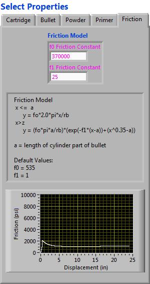
6 (a) (b) (c) (d) (e) Figure 5. "Select Properties" pages for "Forward Calculation" also used in other calculation modes 6

7 (a) (b) (c) (d) Figure 6. "Calculation Output" pages for "Forward Calculation" 7

The sensitivity analysis mode is selected by clicking on the tab labeled "Sensitivity Analysis" under the label "Calculation Mode and Program Control".

8 The sensitivity analysis mode is selected by clicking on the tab labeled "Sensitivity Analysis" under the label "Calculation Mode and Program Control". The window shown in Figure 4(b) will then appear. In this window, the property that is to be varied is selected by clicking on the button below the property name. Only one selection is allowed for each calculation. Definitions of the property names can be pulled up by clicking on the "Get Definitions" button (See Figure 4(b)). To run the desired sensitivity analysis, select the cartridge, bullet, and powder properties on the respective windows under "Select Properties", then click on the "Run Calculation" button. Outputs from the sensitivity analysis calculation are found on the "Sensitivity" page of the "Calculation Output" group. Figure 7 shows example output calculations. Note that there are two additional controls on the "Sensitivity" calculation output page: 1) "Percent Change" and 2) "Select P(t) Location". The "Percent Change" input is set by the user to the desired property percent change. This number can be any reasonable positive or negative real number. The "Select P(t) Location" control is a drop-down menu where the x-location for the P(t) calculation can be selected. These controls do not take effect until the "Run Calculation" button is clicked. The first graph on the "Sensitivity" page shows the pressure-time curves for two conditions, one with the selected property not changed, and the other curve with the selected property changed by the amount determined in the "Percent Change" box. In the second graph the normalized derivative, of P(t) with respect to the selected property, is plotted. In this graph, it can be seen where in time the parameter change has the greatest effect on the P(t) curve. Also shown are the maximum pressure and muzzle velocity before and after the property change. (a) (b) Figure 7. Input selection (a) and output calculations (b) for sensitivity analysis calculation mode 8

3.3 Inverse Calculation AnalyzeLoad(2.x) and AnalyzeLoad(3.x) only 3.3.1 Inverse Calculation - Friction This calculation mode is offered to help the shooter determine the unknown effects of

9 3.3 Inverse Calculation AnalyzeLoad(2.x) and AnalyzeLoad(3.x) only Inverse Calculation - Friction This calculation mode is offered to help the shooter determine the unknown effects of bullet/barrel friction and other unknown effects which can be lumped into the bullet/barrel friction such as energy losses from heat transfer into the barrel. The underlying mathematical process is a polynomial fit to the interior ballistics model by least-squares minimization. In this inverse calculation mode, the input data for fixed cartridge, fixed barrel length (fixed gun), fixed bullet weight, and fixed powder type, are powder weight, and muzzle velocity. The least-squares fit adjusts the value for the bullet/barrel friction constant, f0. When in the inverse calculation mode, the powder type must be selected on the "Inverse Calculation" page under the "Calculation Mode and Program Control" label. To select this mode, the "Inverse Calculation" tab under the "Calculation Mode and Program Control" label must be clicked and then the friction tab on that page is also selected. Input conditions are entered on this page and output is found under the "Calculation Output" label on the page with the tab labeled "Inverse-Frict" for AnalyzeLoad(2.x) and Inverse Friction for AnalyzeLoad(3.x). An example output is shown in Figure 8. The plot on the "Inverse-Frict" output page shows the measured velocity plotted against the best fit calculated velocity. For a good fit, data points should lie on, or close to, the line shown in the plot. The best fit value for the bullet/barrel friction constant is given numerically. If the user desires to keep and reuse the fit value, the button "Press to Save" must be clicked. This will cause the fit value to replace the corresponding values on the "Friction" page under the "Calculation Mode and Program Control" label. This value can only be saved by pressing the "Press to Save Current Settings" button on the "Forward Calculation" page under the "Calculation Mode and Program Control" label as discussed in section 3.1 above. The limits on the graphs can be adjusted by changing the values for "v-lower limit" and "v-upper limit". This calculation mode can take a few minutes to execute. (a) (b) Figure 8. Input selection (a) and output calculations (b) for inverse calculation mode 9

10 3.3.2 Inverse Calculation - Burn Rate Constants This mode of calculation is offered in the advent that some propellant properties may not be known, or are believed to be inaccurate for the shooting conditions and propellant lot or batch being used. The underlying mathematical process is a Levenberg Marquardt least-squares fit to the interior ballistics model. In this inverse calculation mode, the input data are cartridge type, barrel length, bullet weight, powder weight, and muzzle velocity for a selected powder type. The least-squares fit adjusts values for i) propellant burn rate coefficient (ul) and ii) propellant burn rate exponent (alfa) until the "best fit" to the input velocity measurements is achieved. When in the inverse calculation mode, the powder type must be selected on the "Inverse Calculation" page. To select the inverse calculation mode, the "Inverse Calculation" tab under the "Calculation Mode and Program Control" label must be clicked. The "Burn Rate" tab on this page is also clicked and the powder type selected. The other input properties are entered on this page and the output is found under the "Calculation Output" label on the page with the tab labeled "Inverse-Burn Rate". An example output is shown in Figure 9. The plot on the "Inverse-Burn Rate" output page shows measured velocities plotted against best fit calculated velocities. For a good fit, data points should lie on, or close to, the line shown in the plot. The best fit values for burn rate coefficient and burn rate exponent are given numerically. If the user desires to keep and reuse these fit values, the button "Press to Save" must be clicked. This will cause the fit values to replace the corresponding values on the "Powder" page under the "Calculation Mode and Program Control" label. The propellant properties are permanently saved and will come up the next time the program is run and the corresponding propellant selected. The limits on the graphs can be adjusted by changing the values for "v-lower limit" and "v-upper limit". Other controls on this page should be left with their default values unless the user has sufficient background in least-squares fitting of arbitrary functions to make appropriate changes. This mode of calculation can take up to a few minutes to execute. This inverse calculation mode can also be used to find measurements that are out-of-family. The example calculation shown in Figure 10 uses the same input data as in Figure 9 except the muzzle velocity for the second cartridge (.243 Win) is changed from 2806 ft/sec to 3425 ft/sec. It is readily seen in Figure 10 (b) that the new value is out-of-family, and is concluded to be in error. It should be noted that the results of both inverse calculation modes are only as good as the input measurement data. If there are significant errors in muzzle velocity measurements, or the wrong barrel length is input, or other errors exist in the data, the calculated barrel friction or propellant properties will be in error. One clue that there may be error in the input measurements is if the output values are negative or "NaN" is displayed in place of a numerical output. This can happen if one or more measured muzzle velocities are unrealistically high or low. The best practice is to repeat the calculation three or more times with different input values and then average results for calculated properties. If the user is interested in having AnalyzeLoad customized to fit other parameters such as those listed on the "Sensitivity Analysis" page, the Box Elder Innovations software developers can be contacted through the website at Exterior Ballistics - AnalyzeLoad(1.0) and AnalyzeLoad(3.0) Input for the exterior ballistics module is found by clicking the Exterior Ballistics tab in the Calculation Mode and Program Control Region of the main user interface as shown in Figure

11 (a) (b) Figure 9. Input selection (a) and output calculations (b) for inverse calculation mode (a) (b) Figure 10. Least-Squares fit showing out-of-family 243 Win measurement (circled value in graph) 11

Figure 11. Input for Exterior Ballistics model Generally, this module will be run after the interior ballistics module is run first. Properties and shooting conditions must be manually input.

12 Figure 11. Input for Exterior Ballistics model Generally, this module will be run after the interior ballistics module is run first. Properties and shooting conditions must be manually input. Note that the Scope Offset (in), Scope Angle est., and the Shooting Angle (deg) are defined in the diagram on the lower right hand corner of the main user interface. It is not necessary to run the interior ballistics model first, before running the exterior ballistics model, but the user must remember to input all parameters needed for the exterior ballistics model. If this is not done, the program can crash, or most certainly give erroneous results. There are additional input parameters on the Calculation Output page, y(x) or Trajectory y(x) for AnalyzeLoad(3.x). There are two numerical inputs, Select Distance (yd) and Select Height (in), needed for computing the Sight-In trajectory. These also must be properly input into their respective fields for the exterior ballistics model to run properly. The graphical outputs show the trajectory for the Sight-In conditions, and the Trajectory Relative to the Line-of-Sight when the gun is fired at the angle input in the Shooting Angle (deg) field. The user will note that the apparent trajectory when shooting at angles different from horizontal can differ considerably from horizontal shooting as given by the Sight-In conditions. The Sight-In Velocity is also shown graphically on the y(x) page as an additional output. Figure 12 shows typical results. The plot labeled Trajectory Relative to Line-of- Sight is what the shooter will expect when shooting at the angle defined in the input, Shooting Angle (deg). The max rise (in), distance at max rise (yd), and point blank range (yd) are shown on the Trajectory Relative to Line-of-Sight plot. Note that the maximum rise is greater when shooting uphill at a 30 deg angle than when shooting horizontally as shown in the Sight-In plot. The point blank range (yd) is defined as the distance where the bullet remains within +/- max rise (in). 12

Referring to Figure 13, there are three save trajectory buttons below the top graph labeled Save Trajectory 1, Save Trajectory 2, and Save Trajectory 3.

13 Referring to Figure 13, there are three save trajectory buttons below the top graph labeled Save Trajectory 1, Save Trajectory 2, and Save Trajectory 3. These buttons can be clicked to save up to three different trajectory calculations that can be reviewed on the Review EB Calc tab shown in Figure 12 or Review Exterior Ballistics tab for AnalyzeLoad(3.x). Also note that for AnalyzeLoad(1.x) and AnalyzeLoad(3.x) there are also three save pressure buttons on the P(t) tab that can be used to save up to three different pressure-time curve calculations which can then be reviewed on the Review IB Calc tab as shown in Figure 14. Figure 12. Exterior ballistics calculation output using input parameters as defined in Figure 11 and in this chart just below the top graph. 13

14 Figure 13. Trajectory comparisons for up to three trajectory calculations. 14

15 Figure 14. Pressure-time curve comparisons for up to three interior ballistics calculations. 15

qbal - v1.06 User Manual

qbal - v1.06 User Manual qbal User Manual Page 1 / 12 1 Introduction Qbal is a ballistic simulator for the practice of shooting. All details about the software can be found on the internet at: http://mankonit.free.fr/qbal/