Module 10. Network Simplex Method:

Transcription

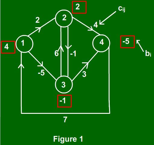
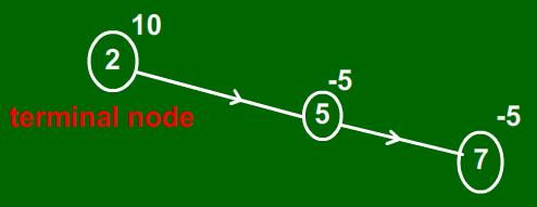
1 Module 10 1 Network Simplex Method: In this lecture we shall study a specialized simplex method specifically designed to solve network structured linear programming problems. This specialized algorithm is called Network Simplex Method (NSM). This method performs the entire simplex method on the network itself. The NSM is generally much faster than the typical simplex method on network linear optimization problem. Network problems whose linear program have 1000 constraints and 30,000 variables can be solved in few seconds by the NSM. Moreover, NSM naturally yields integer network optimization problems); thus one need not restore to the ineffective and time consuming integer programming algorithms (like branch and bound and cutting plane algorithms). Recall minimum cost network flow problem (CP) from previous lecture. Let G=(V,E) be a network in which the arcs are directed and along each arc (i,j) some cost c ij is associated which denotes the cost of transporting one unit of an item form node i to node j. With each node i in G we also associate a number b i representing available supply of an item at source node (if b i > 0) or the required demand for the item at sink nodes (if b i < 0), the transshipment nodes have b i = 0. We shall assume that i V b i = 0 (or total supply equals total demand); else we can add a dummy demand node or sink if i V b i > 0 (or dummy source node if i V b i < 0) and link this dummy node with zero cost arcs to each supply node (or zero cost arcs with each demand node as the case may be). The minimal cost network problem is to find a flow x = (x ij ) such that it solves the following problem. (CP) min subject to m m i=1 j=1 c ij x ij m j=1 x ij m k=1 x ki = b i, i = 1,..., m x ij 0, i, j = 1,..., m Where m denotes the total number of nodes in G or m= V. Problem (CP) is incapacitated, however, if we include the upper bound u ij on flow x ij or 0 x ij u ij constraints then (CP) is called capacitated problem. For example, consider the following network problem. The numbers in box along the nodes are b i -values while the numbers along the directed arcs are c ij -values. The (CP) problem for this network is as follows: min 2x 12 5x x x 23 x x x 41

2 subject to x 12 + x 13 x 41 = 4 x 23 + x 24 x 12 x 32 = 2 x 32 + x 34 x 13 x 23 = 1 x 41 x 24 x 34 = 5 x ij 0 i, j 2 Note that if we write the coefficient matrix A for above problem it is as follows: Note that each column a ij of A is of the form a ij = e i e j where e i and e j are unit vectors having 1 at the i th and the j th position respectively see, 1 0 a 12 = Here when we write a ij it means that (i, j) E with directed arc i j in G. In fact if we carefully examine the constraint structure of a general (CP), we can realize that each column of coefficient matrix A has two non-zero entries exactly, one is +1 and other is -1 because if x ij is a flow from node i to node j then it has a coefficient +1 in the i th node constraint and -1 in the j th node constraint. And since we consider only simple network (hence we do not have multiple arcs in same direction or self loops), this x ij variable will not appear in any other constraint. Remember in chapter 8 too when we were discussing (TP) problems then also we come across absolutely similar situation. In fact (TP) is a special case of (CP). Thus the theory and results for (CP) are same as the one for (TP). In lieu of this we skip proofs of almost all results associated with structure of matrix A in (CP); but encourage you to re look at module 8 and convince yourself that you are all familiar with all results stated below. (1) The matrix A is called node-arc incidence matrix with m rows representing m nodes in G and n columns are n-arcs (directed) in E of G. The rank of the matrix A is m-1. Thus every basis matrix of (CP) is (m-1) x (m-1) submatrix of A. (2) The matrix A is totally unimodular. Consequently each basis matrix B has dot B=±1, and every extreme point of the feasible set is integer-valued for integer right-hand-side b vector in (CP). (3) The scalars y ij s which appear in the linear expression By ij = a ij (remember in simplex

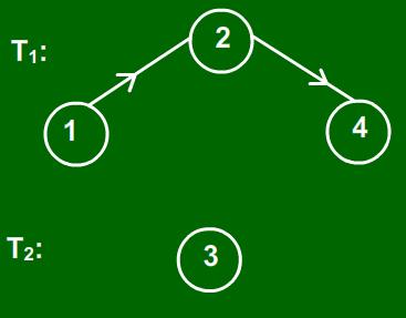
3 3 method for LPP, we have By j = a j ), can take values 0 or ±1. Thus, any column a ij can be obtained by simple addition and subtraction of basic variables columns. The value of each y ij can simply be determined from the network itself. We have explained this aspect in Module 8 also. We take a pause here and describe another concept called TREE as we shall be needing it in our subsequent discussion. A tree is a connected graph having no cycles. Let G=(V,E) be a directed network. A spanning tree T of G is a tree that includes every node of G. Figure 3: Some spanning trees of G. We list below some properties of spanning tree (without proofs). this properties are simple to understand through some simple examples. Property 1: Let T be a tree having m( 2) nodes and (i,j) be an arc in T. If we disconnect (or remove) this arc (i,j) from T but leaving the nodes i and j in T then T gets decomposed into two trees T 1 and T 2. For example, if we take a spanning tree in Figure 3 say Suppose we delete the arc (2,3) but retain the nodes, then it results in Consider a spanning tree for some underlying graph G say as follows. Suppose we remove only arc (2,3) from this tree then it results in two trees. Property 2: A proper tree has at least two leaf nodes (nodes with degree 1). For instance if we see proper tree T in figure 4, it has four nodes as leaf nodes while T 1 and T 2 in figure 5 have 2 leaf nodes each. Property 3: A tree having m nodes has (m-1) arc. This property can easily be seen in all above examples of trees. These fundamental properties help to establish the following equivalent characterizations of a tree. Resul: Let T be a tree. The following are equivalent (a) T is connected and has no cycles. (b) T is connected and has (m-1) arcs. (c) T has (m-1) arcs and has no cycles. (d) T is connected and disconnecting any arc from T results in two trees. (d) T has no cycle and adding any new arc to T (but no new node) results in a unique cycle. To illustrate point (e), consider a network in figure 2 and its spanning tree (say first one) in

4 figure 3. Suppose we add an arc (1,3), which was an arc in G, in this spanning tree it yields 4 Resulting a cycle (note when we say cycle we do not take into consideration the directions of arcs). We are now ready to discuss NSM, but with just one more observation. Recall that the simplex method for LPP always starts with a full rank constraint matrix while herein (CP) the rank of A is m-1. So, we add an artificial variable so that the rank of resultant matrix is m. We introduce this artificial variable (or in one case it is an artificial flow) to say m th node (in fact any one of G). This leads to the constraint matrix (A,e m ). The artificial arc beginning at node m is terminating in space. The node m is then called root node. Any basic feasible solution of (CP) must contain m linearly independent columns (or flows variables) hence the artificial variable appear in every basic feasible solution. For example, suppose we take node 4 as a root node in Figure 2. and suppose the spanning tree of this rooted graph is as follows. This is a rooted spanning tree. The matrix corresponding to rooted spanning tree is as follows. Remark:- A rooted spanning tree corresponds to a basis matrix of (A,e m ). The converse is also true. Any basis matrix B of (A,e m ) is a node-arc incidence In nut shell we have a result that B is a basis matrix of a minimum cost flow problem on a connected directed graph having one root arc if and only if B is the node-arc incidence matrix of a rooted spanning tree of G. Network Simplex Method (I) To obtain initial basic feasible solution(ibfs) Recall the constraint equations of (CP) We assume that m i=1 b i = 0. xij x ki = b i, i = 1,..., m. {j (i, j) E} {k (k, i) E} (1) x ij 0, (i, j) The BFS s of (1) is in 1-1 correspondence with the set of spanning trees of underline network G. Let T be a spanning tree. Then T has at least one terminal (or leaf) node. Suppose this node is node i. The node-arc incidence matrix of T has only one non-zero entry in the i th row. This entry is either +1 or -1. If this entry is +1 then there is an outgoing arc (i,j) in T and if the entry is -1 then there is an incoming arc (j,i) incident at node i in T. Then, set

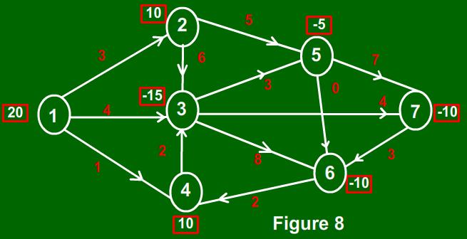
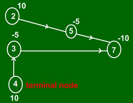
5 5 b i if (i, j) is an arc in T x ij = b i if (j, i) is an arc in T Delete node i and the arc (i,j) or (j,i) whatever the case may be. Replace the value b j at node j by b j + b i. The resultant graph is also a tree. So, we can repeat this process (m-1) times (note that T has m-1 edges/arcs) to get the BFS corresponding to T. Consider the following network. The numbers in box are b i values and the numbers along arcs are c ij values. Note that b i = 0. Let the following spanning tree T of G be the initial tree with which we start the NSM. Note that T has 6 arcs and 7 nodes. We take node 1 as a terminal/leaf node of T.So, i=1 and j=3. Set x 13 =20. Delete node 1 and replace b 3 by b 3 + b 1 = =5. The resultant tree is as follows. We take node 6 as next leaf node. So i=6 and j=3. Set x 63 = b 6 = 10, and replace b 3 by b 3 + b 6 =5-10= -5. The next tree is as follows Set x 43 = b 4 = 10 and replace b 3 by b 3 + b 4 =5. Set x 37 =5 and replace b 7 =-10+5= -5 Set x 25 =10, and replace b 5 by b 5 + b 2 =5. Thereafter set x 57 =5. If we depict the initial flow vector in the original network G (figure 8), then we have the following network. The numbers in bracket along the arcs is ordered pair (c,x), so, along arc 1 4, the pair (1,0) means c 14 =1 and x 14 =0. For this IBFS x = (x ij ), the cost of flow is i j c ij x ij =4x20+2x10+5x10+7x4+4x5+8x10=285. To check optimality of Flow vector This may or may not be the minimum (or optimal) cost. We need to check if the flow vector x= (x ij ) is an optimal one and if it is not an optimal solution then how one can optimize it? To answer these questions, as usual, we restore to the concept of duality in network problem. We urge you to recall from LPP or TP duality that the reduced cost vector

6 6 z ij c ij = wa ij c ij. where w(=c B B 1 or wb = c B ) is a complementary dual variable. Here, we get z ij c ij = w(e i e j ) c ij = w i w j c ij For (i, j) T (basic cells), we have, w i w j = c ij Since any one of the constraints of (CP) can be discarded as a redundant constraint, we can assign value 0 to any one of the dual variables. Then we solve for other dual variables as follows. w p c pq if we have arc (p, q) in T w q = w p + c qp if we have arc (q, p) in T Thus, if w p is known then we can compute w q. For example, go back to figure 10. Recall the initial BFS tree is as follows Let w 7 =0 Then w 5 = w 7 + c 57 = 7 w 3 = w 7 + c 37 = 4 w 2 = w 5 + c 25 = 12 w 1 = w 3 + c 13 = 8 w 4 = w 3 + c 43 = 6 w 6 = w 3 c 36 = 4 All these calculations can easily be done on the network tree itself. Thereafter we go back to main network in figure 10 and compute the reduced cost along all those arcs (i,j) which are not in the tree network. z ij c ij = w i w j c ij So, we have z 12 c 12 = = 7 z 14 c 14 = = 1 z 23 c 23 = 2 z 35 c 35 = 6, z 56 c 56 = 1 z 64 c 64 = 12, z 76 c 76 = 1

7 7 Since some z ij c ij > 0, so current x is not an optimal one. To obtain Improved BFS If z rs c rs is maximum positive value then the arc (r,s) enters in the basis (or tree here). This leads to a formation of a unique cycle in the resultant network T {(r, s)}. Cycle basically means that the arcs form a linearly dependent set. So, arc can be expressed as a linear combination of the columns of node-arc incidence matrix of T. That is, a rs = By rs where B is the node-arc incidence matrix of T. Now, we have earlier observed that the vector components can be ±1 or 0. Consider the cycle formed in T on introduction of arc (r,s). Focus on the orientation of arcs in C. Then note y pq = +1 if (p,q) is reverse to (r,s) = 1 if (p,q) is in the same direction of (r,s). Then identify =min (x pq ), where (p,q) is arc in reverse direction to (r,s). The new BFS is then constructed as follows x ij if (i, j) C x new = x ij + if (i, j) has y ij = 1 x ij if (i, j) has y ij = + 1 For example, go back to figure 11. z 23 c 23 = +2 is most positive value so arc (2,3) enters into T resulting in the following graph. This leads to a cycle shown in red above. Taking the direction of (2,3), we find that arcs (5,7) and (2,5) are in reverse orientation of cycle. Thus, = min {x 57, x 25 }=5=x 57 Therefore arc(5,7) leaves the tree. We get a new tree with flow x updated along the arcs. We again compute the dual variables w by setting w 7 = 0. The w- values are as follows. w 7 = 0, w 3 = w 7 + c 37 = 4, w 4 = 6, w 6 = 4, w 2 = 10, w 5 = 5; and the reduced costs for non-basic arcs are as follows

8 8 z 12 = c 12 = 5, z 14 c 14 = 1, z 35 c 35 = 4, z 64 c 64 = 12, z 76 c 76 = 1, z 57 c 57 = 2, z 56 c 56 = 1 So, arc(7,6) enters in the tree and one can verify that arc (3,6) leaves the tree. We have a new tree as follows. Again we can check the optimality of flow x. In this way we repeat the procedure till we achieve an optimal solution (or optimal flow vector x) for the problem (CP). All the computations can easily be done on the network itself and all of them are fairly intuitive. We encourage you to complete the above example and find the optimal (or minimum) spanning tree for the problem. Though here we are skipping the discussion on a capacitated minimum cost network flow problems and unbalanced problems but then those will involve routine extensions/generalizatios of NSM. We leave it for you to explore the same in some good Network optimization books/chapters or on www.

9 9

10 10

11 11

12 12