Light field editing and rendering

Transcription

1 Light field editing and rendering Matthieu Hog To cite this version: Matthieu Hog. Light field editing and rendering. Computer Vision and Pattern Recognition [cs.cv]. Université Rennes 1; Rennes 1, English. <NNT : 2018REN1S064>. <tel > HAL Id: tel Submitted on 19 Mar 2019 HAL is a multi-disciplinary open access archive for the deposit and dissemination of scientific research documents, whether they are published or not. The documents may come from teaching and research institutions in France or abroad, or from public or private research centers. L archive ouverte pluridisciplinaire HAL, est destinée au dépôt et à la diffusion de documents scientifiques de niveau recherche, publiés ou non, émanant des établissements d enseignement et de recherche français ou étrangers, des laboratoires publics ou privés.

2 THESE DE DOCTORAT DE L'UNIVERSITE DE RENNES 1 COMUE UNIVERSITE BRETAGNE LOIRE ECOLE DOCTORALE N 601 Mathématiques et Sciences et Technologies de l'information et de la Communication Spécialité : Informatique Par Matthieu HOG Light Field Editing and Rendering Thèse présentée et soutenue à Rennes, le 21 Novembre 2018 Unité de recherche : INRIA Rennes - Bretagne Atlantique et Technicolor R&I Rapporteurs avant soutenance : Bastian GOLDLUECKE Pascal MONASSE Professor, University of Konstanz Professor, Ecole des Ponts ParisTech Composition du Jury : Président : Luce MORIN Professor, INSA Rennes Examinateurs : Frederic DEVERNAY Researcher, Amazon Bastian GOLDLUECKE Professor, University of Konstanz Pascal MONASSE Professor, Ecole des Ponts ParisTech Aljosa SMOLIC Professor, Trinity College Dublin Dir. de thèse : Christine GUILLEMOT Research Director, INRIA Rennes Neus SABATER Researcher, Technicolor R&I

3

4 Acknowledgments I want to first and foremost express my gratitude to my PhD advisors Christine and Neus who not only guided me with their expertise, but also knew when to give me autonomy and when to push me to write. I couldn t have hoped for better mentors. I would like to re-iterate my gratitude to the defense committee for their time, positive feedback, interesting questions and discussions. Thank you to the 3rd floor team at Technicolor, especially Arno, Artem, Benoist, Didier, Frederic, Guillaume, Laurent, Mitra, Mozhdeh, Olivier, Paul, Remy, Tristan, Valérie and Valter. These 3 years have been really fun, and I ll miss your good company. I also want to thank the PhD and postdoc dream-team, especially Dmitry, Fatma, Guillaume, Jean, Juan, Julia, Martin and Salma. Thank you for all the good laugh, happy lunch time and also getting me out of my cave sometimes. Finally, I thank my family, especially Marie, for their endless support and love.

5

6 Contents Contents 2 List of figures 2 List of tables 4 List of algorithms 5 Résumé En Français 7 I Opening 15 1 General Introduction Context Motivations and Goals Thesis Structure and Contributions Background in Light Field Imaging Formal Definition Acquisition and Sampling Applications II Light Field Image Rendering 35 3 An Image Rendering Pipeline for Focused Plenoptic Cameras Introduction Related Work Plenoptic Image calibration Proposed Depth Estimation Method Rendering using a Focus Map Experiments Conclusion Light Field View Synthesis with Recurrent Neural Networks Introduction Related Work LSTMs for View Synthesis Experiments Conclusion

7 III Light Field Editing 69 5 Light Field Segmentation Using a Ray-Based Graph Structure Introduction Related Work Ray-based Graph Structure Energy Function Experiments Conclusion Super-rays for Efficient Light Field Processing Introduction Related Work Super-ray Light Field Over-Segmentation Super-ray Applications Conclusion Dynamic Super-Rays for Efficient Light Field Video Processing Introduction Related Work Dynamic super-rays Experiments Conclusion IV Closing General Conclusion Summary Future work and Perspectives Appendix A Author s publications 119 Appendix B List of Notations 121 Appendix C Additional Results for Chap Bibliography 139 2

8 List of Figures 1.1 Lenticular print principle Example of depth estimation from light fields Example of post-shot image rendering Example of light field capturing devices Plenoptic function vs the two-plane parametrization Example of a light field captured with a camera array How a plenoptic camera captures a light field Example of light field captured with a plenoptic camera Example of refocusing The two plenoptic camera designs Proposed pipeline to process a raw light field captured with a focused plenoptic camera Estimated subaperture image from a focused plenoptic camera Micro-lens array calibration parameters A white plenoptic image is a sum of three 2D cosine Comparison of a white image synthesized with our model versus a real white Raytrix image Comparison with Dansereau s calibration Calibration on a natural raw plenoptic image The stereo focal stack computation Projection of a scene point visible on two microlens images Results on the donkey dataset Comparison of our depth maps with R11 test images Comparison of our depth maps using the Georgiev s dataset R11 all-in-focus rendering on test image Andrea Refocusing with and without splatting comparison A typical LSTM cell Our LSTM cell Visualization of the LSTM memory state Interpolation with wide baseline Visualization of the LSTM memory state for wide baseline View synthesis results for a deep hierarchical approach Comparison with the Proposed light field representation Illustration of the over-connectivity problem Light field segmentation results on synthetic light fields Visualization of the graph nodes for the dataset Tsukuba Experiments with our synthetic, sparsely sampled light field

9 5.6 Light-field segmentation results on real datasets Example of angular patches The super-ray assignment step The super-ray update step Average displacement of the super-ray centroids with respect to the number of iterations Different super-rays evaluation metrics across different parameters for a synthetic scene Comparison of super-rays versus independently merged super-pixels Super-rays for a sparsely sampled light field Super-rays for a densely sampled light field Graph-cut segmentation using our super-rays Angular aliasing comparison Refocusing on a sparsely sampled dataset Illustration of our algorithm in a simple case Duper-ray neighborhood Dynamic super-rays for a few frames and views Over-segmentation comparison with the state of the art

10 List of Tables 3.1 Calibration errors comparison with the state of the art Image quality metrics for the compared approaches Segmentation accuracy comparison Comparison of the total segmentation running times with the state of the art Super-rays segmentation accuracy

11 List of Algorithms 1 Super-ray algorithm Dynamic super-ray algorithm

12 Résumé En Français Contexte Que ce soit pour les films, les jeux vidéo ou même la photographie, il y a un intérêt particulier à donner une impression de profondeur, de géométrie au contenu que nous souhaitons capturer et diffuser. Au cours de cette dernière décade, plusieurs domaines de recherche et de l industrie se sont penchés sur le problème de la capture et de la restitution de contenus avec des informations géométriques supplémentaires, pas nécessairement présentes ou faciles à obtenir à partir d une imagerie 2D classique. Les films 3D stéréoscopiques illustrent bien cet investissement. En moins de 10 ans, ils sont devenus une norme dans l industrie du film à gros budget. Le nombre de films 3D produits par an est passé de 6 en 2007 à 52 en 2016 et le nombre d écrans 3D dans le monde est passé de en 2012 à en 2016 [1]. Un autre exemple est le contenu de réalité virtuelle (VR). L amélioration récente du prix et de la qualité des casques VR (par exemple, le HTC Vive, Daydream project, Oculus Go pour n en citer que quelques-uns) ouvrent un nouveau marché de production d images et de vidéos stéréoscopiques et 360. Une partie de ce type de contenu est capturée à partir de scènes réelles, utilisant souvent des systèmes multi-caméras complexes, tels que le court métrage MPC VR Catatonic 1, ou des configurations plus accessibles 2. Un dernier exemple, peut-être assez différent des deux autres, est celui des smartphones. Motivés par le fait que nous atteignons les limites de résolution des capteurs et aussi des performances des optiques portables, les smartphones de la génération actuelle ont désormais une paire (ou plus) de caméras et utilisent du traitement d image pour produire la photographie finale. Il est intéressant de noter que l application la plus populaire pour ces images stéréo est de produire un flou artistique (bokeh) pour donner une impression de profondeur aux photographies, une tâche impossible pour un objectif portable classique doté d une ouverture trop étroite. Pour les médias que nous avons mentionnés, un nouveau défi à résoudre semble être la capture et le rendu de contenus augmentés en 3D. Malgré les dernières avancées en matière d imagerie tridimensionnelle, il s agit toujours d un problème qu en partie résolu. Par exemple, la génération des cartes de profondeur pour les films stéréoscopiques nécessite encore beaucoup d interventions humaines, manuelles, fastidieuses et coûteuses. Les films VR sont encore assez coûteux à produire et reposent souvent sur des capteurs actifs pour capturer la profondeur de la scène, ce qui présente certaines limites. Même sur les téléphones haut de gamme, les images générées par les appareils photo doubles sont d une qualité moindre que les appareils photo ordinaires. Les erreurs dans l effet de bokeh mentionné la chaine VR officielle de youtube contient plus de 300 vidéos VR. UCzuqhhs6NWbgTzMuM09WKDQ/videos 7

13 sont particulièrement désagréables, soulignant la nécessité de meilleurs algorithmes de traitement. Dans ce contexte, l imagerie par champs de lumière (light field) est une alternative sérieuse pour gérer de nombreux aspects de la capture d images 3D. Motivation et Objectif Comme son nom l indique, le terme champ de lumière réfère au concept de représentation de la lumière en tant que champ vectoriel. Formellement, il s agit d une description des intensités d une collection de rayons, circulant de, et vers tous les points de l espace. D un point de vue plus grossier, cependant, un champ de lumière est un terme large qui désigne la capture simultanée d une scène à partir de plusieurs points de vue. Dans de nombreux cas, un champ de lumière peut être représenté comme un ensemble de vues décrivant la même région d intérêt. Beaucoup de contenus entrent dans cette définition très générique mais nous nous concentrons toutefois sur un cas particulier, lorsque le champ de lumière est structuré, dans le sens où les vues doivent être prises (approximativement) sur un plan et à une distance régulière les unes des autres. Nous supposons également que le nombre de vues est supérieur à deux. Grâce à ces hypothèses, et contrairement à une image standard, un champ de lumière enregistre de nombreuses informations sur la géométrie d une scène. Cette information peut être récupérée et exploitée pour des traitements ultérieurs. Une première utilisation et peut-être la plus simple des champs de lumière consiste à reconstruire directement différents points de vue de la même scène. Lorsqu il est combiné avec une surface qui rend les rayons capturés par la direction, il est alors possible de simuler un changement de point de vue pour un observateur. Un exemple bien connu de ce principe est celui des impressions lenticulaires, très populaires pour les cartes postales. Des lentilles cylindriques sont placées sur une image imprimée composée de deux (ou plus) images entrelacées avec des points de vue différents ou capturées à un moment différent (Fig. 1). La version moderne de ce principe sont les écrans auto-stéréoscopiques, qui remplacent le papier par un affichage numérique et utilisent des microlentilles pour re-projeter les rayons à la verticale et à l horizontale. Cela permet à un spectateur de percevoir la profondeur et la parallaxe de mouvement sans être équipé d aucun autre appareil. Bien que le résultat de ces affichages puisse être assez surprenant, du fait que le nombre de vues d un champ de lumière est limité, la transition entre les points de vue peut paraître brusque (problème de sous-échantillonage). Cela motive le deuxième exemple d application: synthétiser des points de vue supplémentaires à partir du signal capturé. Dans le cas particulier où les vues sont suffisamment proches, une simple interpolation peut être utilisée pour compenser cet effet. Toutefois, dans le cas où la distance entre les vue est importante, des informations sur la géométrie de la scène sont nécessaires. Parce que nous capturons une scène avec différents points de vue et avec une disposition connue, le mouvement de parallaxe permet une reconstruction 3D passive. Bien que la disposition et le nombre de vues déterminent le type de méthode d estimation de profondeur à utiliser, la redondance des vues du champ de lumière et la régularité de l échantillonnage donnent généralement des cartes de profondeur de haute qualité. Ces cartes de profondeur peuvent alors être utilisées pour générer des modèles 3D ou des nuages de points très denses et précis (exemple de la Fig 2a). Avoir une estimation de profondeur de haute qualité à partir de capteurs passifs est particulièrement intéressant pour l industrie du film 3D, car elle nécessite moins de corrections manuelles. Cela peut également être intéressant dans 8

14 Observers L R L R R L R L Lenticular lenses Printed surface Figure 1: Principe de l impression lenticulaire. Nous montrons un schéma en 2D par souci de simplicité. Deux images différentes L et R sont entrelacées sur une surface imprimée. Les lentilles cylindriques re-projettent les rayons de la surface imprimée selon leur direction. Les observateurs sont à deux points de vue différents et voient respectivement les images A et B. Ce principe peut être étendu sans perte de généralité en 2D. le contexte de la fabrication industrielle, où l inspection d objets est souvent complexe, en gros plan et lorsque des objets non Lambertiens sont examinés. Par exemple, la carte de profondeur de la Fig. 2b serait difficile à obtenir avec une configuration stéréo ou des capteurs de profondeur actifs. Ces informations de géométrie peuvent également être utilisées pour la synthèse des vues, que ce soit en tant que contrainte dure ou relaxée. Ceci est d un intérêt particulier pour les écrans VR, ce qui nécessite un changement de point de vue très fluide pour préserver l expérience utilisateur. Un exemple particulièrement impressionnant de cela est la démonstration Welcome to light field 3. Néanmoins, toutes les applications ne visent pas à fournir plusieurs vues. Comme les rayons capturés d un champ de lumière ont des coordonnées connues, il est possible de reproduire le processus d intégration effectué par une caméra conventionnelle après la capture et avec des paramètres ajustables. Le problème d ouverture synthétique permet ainsi de rendre des images avec différentes profondeurs de champs et plans de mise au point à partir de champs de lumière. Ceci est particulièrement utile dans les situations où la mise au point de la caméra est difficile à ajuster (comme illustré sur la Fig. 3), ou pour produire différents effets à partir d images statiques (comme par exemple changer le plan de mise au point pour produire un effet de découverte). Pour longtemps restées comme un concept théorique, toutes ces applications ont pris de l ampleur dans la recherche et l industrie grâce au développement récent des dispositifs d acquisition de champs de lumière. Par exemple, les caméras plénoptiques ou les matrices de caméras (Fig. 4) sont devenues de plus en plus communes ces dernières années, tant du côté de la recherche que de l industrie. Comme on peut le déduire de par la taille des deux types d appareils, les champs de lumière capturés sont assez différents dans leur échantillonnage. En effet, dans certains cas, le champ de lumière capturé ne peut pas être directement présenté comme un ensemble de vues ou alors les vues sont très éloignées. Cela nous amène au premier problème que nous abordons dans cette thèse: comment traiter et restituer des images à partir de champs de lumière pour des cas particuliers, qui sont difficiles et moins explorés dans la littérature actuelle. Un autre problème est qu il existe une multitude de méthodes et de solutions commerciales 3 9

15 (a) Nuage de point obtenu à partir d un champ de lumière (b) Carte de profondeur obtenue à partir d un champ de lumière Figure 2: Exemple d estimation de profondeur à partir d un champ de lumière. Sur la figure (a) nous montrons le rendu d un nuage de point généré à partir de cartes de profondeur calculées à partir d un champ de lumière [2]. Sur la figure (b), nous montrons la vue originale et la carte de profondeur obtenues à partir d un champ de lumière[3]. La scène capturée est complexe car elle contient des surfaces très spéculaires et est proche du système d acquisition. pour modifier une image ou une vidéo (e.g. Photoshop, GIMP, Adobe Premiere), cependant, peu d options sont disponibles dans le cas de contenu 3D, et encore moins pour les champs de lumière. Pourtant, une interaction à posteriori au rendu (possiblement guidée par un utilisateur) ouvre la voie à des applications plus avancées. Ceci est le deuxième sujet abordé lors de cette thèse: comment interagir avec les champs de lumière avant toute modification ultérieure. Plus précisément, le problème est double. Puisque le contenu décrit par le champ de lumière est redondant, nous nous attendons à ce qu une modification soit cohérente d une vue à une autre. Dans certains cas également, la quantité d informations capturées est problématique si la méthode d interaction ne s adapte pas au volume de l entrée. Comme contrainte supplémentaire, nous avons essayé de ne faire aucune hypothèse sur la densité d échantillonnage des champs de lumière capturés. Et la plupart des approches proposées ne sont pas liées à un type spécifique de périphérique. Nous avons également essayé de garder les méthodes aussi peu complexes que possible pour pouvoir les utiliser dans un contexte industriel. Résumé des Contributions Les contributions de cette thèses sont organisées en deux parties, correspondant aux deux problématiques mentionnées. La partie II présente deux travaux liés à la première question de recherche que nous avons mentionnée: comment produire des images à partir de champs de lumière? Il contient deux 10

16 (a) La photo n est pas focalisée sur la région d intérêt. (b) La photo est focalisée sur la région d intérêt. Figure 3: Exemple de rendu d image après la capture. Dans certaines situations, ajuster le plan de mise au point est difficile. Sur la figure (a), nous montrons la photo que l on obtiendrait probablement avec une caméra conventionnelle, dans ce scénario dynamique. Mais comme cette photo a été rendue à partir d un champ de lumière, il est possible de régler le plan de mise au point après que la photo ait été prise, comme illustré sur la figure (b). chapitres qui peuvent être résumés comme suit. Chapitre 3 : Dans ce premier chapitre de contribution, nous présentons un pipeline complet pour traiter le type particulier de champs de lumière produits par les caméras plénoptiques focalisées. En particulier, nous proposons un nouvel algorithme de calibration entièrement dans le domaine de Fourier, un nouvel algorithme pour le calcul de cartes de profondeur utilisant une pile focale stéréoscopique et enfin, un algorithme de rendu d image basé sur la profondeur, capable de produire des images nettes de partout. Les algorithmes proposés sont rapides, précis et n ont pas besoin de générer des images de sous-ouverture ou des images de plan épipolaire, ce qui est capital pour les caméras plénoptiques focalisées. Le pipeline a été testé sur plusieurs caméras plénoptiques et les images rendues étaient d une qualité comparable à l état de l art, même pour des solutions commerciales. Chapter 4 : Ce court chapitre tente de résoudre le problème de la synthèse des vues intermédiaires à partir d un ensemble de 4 vues seulement. Les réseaux neuronaux récurrents (RNN) sont utilisés pour déduire de manière itérative la couleur la plus probable de la vue à synthétiser, à partir des 4 images d entrées re-projetées sur différents plans de profondeur. L approche est nouvelle, présente une très faible empreinte mémoire et peut être utilisée sur des scènes présentant toutes sorte de disparités. Nous montrons que l approche se comporte comme prévu et fournit des résultats de bonne qualité dans un cas d usage limité. Cependant, nous montrons également que, dans son état actuel, la méthode ne se généralise pas facilement et nous donnons des indications pour améliorer la méthode. Ensuite, la partie III regroupe les travaux liés au problème de l édition des champs de lumière. Le but global de cette partie est d assigner des labels pertinents à chaque rayon du champ de lumière. Chapter 5 : Dans ce chapitre, nous nous intéressons à la segmentation au niveau pixel des champs de lumière, faite de manière interactive. Plus précisément, nous nous concentrons sur l utilisation de techniques bien connues de type champs aléatoires de Markov (Markov Random Field) pour attribuer, à partir d un ensemble épars d annotations utilisateur, un label d objet à chaque rayon d un champ de lumière. Le 11

17 (a) La caméra plénoptique Lytro Illum (b) La matrice de caméra de Technicolor Figure 4: Exemples de système d acquisition de champs de lumière. Sur la figure (a), nous montrons une caméra Lytro Illum qui ressemble à une caméra réflex standard. Sur l image (b) est montrée la matrice de caméra utilisée à Technicolor [2], composée de 16 caméras video. plus grand obstacle à l adoption des champs de Markov pour le traitement des champs de lumière est le grand volume de données en entrée, qui rend rapidement impossible toute tâche d optimisation basée sur ce principe. Pour aborder ce problème, nous introduisons une nouvelle représentation basée graphe qui exploite la redondance dans l espace des rayons afin de réduire la taille du graphe avant tout calcul intensif. Nous proposons ensuite un algorithme de segmentation interactive du champ de lumière par coupe de graphe qui utilise cette structure de graphe. Ceci garantit la cohérence de la segmentation entre toutes les vues. Nos expériences avec plusieurs ensembles de données montrent des résultats proches de la vérité terrain, compétitifs avec les méthodes de segmentation de champs de lumière de l état de l art en terme de précision et avec une complexité nettement inférieure. Elles montrent également que notre méthode fonctionne bien sur des champs de lumière à échantillonnage dense et parcimonieux. Nous montrons également un exemple de la façon dont la segmentation obtenue peut être utilisée pour supprimer un objet d une scène capturée. Chapter 6 : Pour les champs de lumière plus volumineux, l énorme quantité de données de grande dimensionalité pose des problèmes à l édition interactive. Afin de permettre le traitement des champs de lumière avec une complexité raisonnable, nous abordons dans ce chapitre le problème de la sur-segmentation des champs de lumière. Nous introduisons le concept de super-rayon, qui est un regroupement de rayons dans et à travers des vues, en tant que composant clé d un pipeline de traitement de champ de lumière. L approche proposée est simple, rapide, précise, facilement parallélisable et ne nécessite pas d estimation de profondeur dense. Nous démontrons expérimentalement l efficacité de l approche proposée sur des jeux de données réels et synthétiques, pour des champs de lumière échantillonnés de manière dense et éparse. Comme les super-rayons capturent une information de géométrie grossière, nous présentons également comment ils peuvent être utilisés pour la segmentation de champ de lumière en temps réel et la correction du sous-échantillonage angulaire qui apparaît lors de la refocalisation de champs de lumière épars. 12

18 Chapter 7 : Ce dernier chapitre de contribution est la suite logique du chapitre 6. Nous nous appuyons sur notre travail de super-rayons pour proposer la première approche de la sur-segmentation de champs de lumière vidéo, appelée super-rayons dynamiques. Cette approche peut être vue comme des superpixels temporellement et angulairement cohérents. Notre algorithme a la même qualité que les super rayons statiques et est également efficace en terme de mémoire en ce qui concerne le nombre de trames chargées simultanément. En tirant parti de la puissance de calcul des cartes graphiques, nos résultats indiquent des performances proches du temps réel. 13

19 14

20 Part I Opening 15

21 16

22 Chapter 1 General Introduction 1.1 Context I ll never work without 3D again, even for small dialog scenes. I love the whole process. 3D opens up the universe of even a small dialog scene [...] Ridley Scott, film director and producer (Alien, Blade Runner,...) May it be for movies, video-games or even photography, it is clear that there is a particular interest to give a sense of depth, of geometry to the content we wish to capture and deliver. This makes sense, as after all, we have two eyes, we can move, we can focus our gaze on a particular object, and as such, stereo disparity, motion parallax, focus blur are all important geometric cues our visual system relies on. In the last years, several research and industry fields have paid attention to the problem of capturing and restituting content with this extra geometrical information, not necessarily present or easy to obtain from mainstream, 2D imaging. A great illustration of this investment are 3D stereoscopic movies. In less than 10 years, they became a standard in the (high-budget) movie industry. The number of 3D movies produced per year rose from 6 in 2007 to 52 in 2016 and the number of 3D worldwide screen jumped from in 2012 to in 2016 [1]. Another example are contents for Virtual Reality (VR). The recent improvements in quality and mass production of cheap head mounted displays (e.g. the HTC Vive, Daydream project, Oculus Go to mention only a few) open up a new market for 360 -stereoscopic images and videos. Some of this content is captured from real scenes often using heavy multi-camera systems, such as the MPC VR short movie Catatonic 1, or more accessible setups 2. A last example, perhaps quite different from the other one, are smartphones. Motivated by the fact that we are reaching the limits of sensors resolution and optical system that can be packed inside, current generation smartphones now embeds a pair of cameras and use image processing to produce the final image. Interestingly, the most popular application for these stereo images is to produce an artistic defocus blur (bokeh) to give a sense of depth to photos, an impossible task for a regular smartphone camera that typically has a narrow aperture The youtube official VR channel has more than 300 VR videos UCzuqhhs6NWbgTzMuM09WKDQ/videos 17

23 It is tempting to affirm that this taste for 3D cues in media is recent, but if we take a brief overview of how we save and visualize events, we see that this idea is perhaps part of a long chain of innovation focused on a wider goal: improving the capture and the restitution of events to make it closer to the natural, volumetric perception we have. The first challenge that has been solved is to take flat photos that actually look like the original scene. Early 16 th century improvements of the age-old pinhole camera with lenses and diaphragms and the plethora of light-sensitive materials proposed during the 17 th and early 18 th century, made possible to build the very first cameras. By the end of the mid-19 th century, the Daguerreotypy process was a wide-spread, commonly adopted mean of photography. Interestingly, the first stereoscopic photographs were also produced during this time and were quite popular. Color photography process came near the end of the 19 th century to provide long-lasting colorful photos. The second milestone was to introduce movement in pictures. The end of the 19 th century notably saw the creation of the first moving picture acquisition, with continuous improvements of the frame rate and image quality. The third task was to make photos and video easy to capture and modify. This was made possible by first, the invention of digital sensors, i.e. the Nobel-price-wining CDD and later the CMOS, in the late 60s, second by the democratization of cheap and efficient electronics for smartphones and cameras between 1990 and 2010, and third, by the development of image editing software, allowing to change a shot after its capture. While this progress transformed the way we produce and consume media, the captured signal did not fundamentally changed: it is still an image projection on a photo-sensible material. Nowadays, if we take the example of media we mentioned, the new challenge to solve seems to be the capture and rendering of 3D-augmented contents. Despite the latest advances in 3D imaging, this is still a partially-solved problem. For instance, generating the depth maps for stereoscopic movies still requires a lot of tedious, expensive and manual human interventions. VR movies are still quite expensive to produce and often rely on active sensors to capture the depth of the scene, which have some limitations. Even on high-end phones, the images generated by dual cameras are still worse than normal cameras. Errors in the mentioned bokeh effect are particularly unpleasant, stressing the need for better processing algorithms. In this context, light fields imaging is a serious proposition to handle numerous aspects of 3D image capture. 1.2 Motivations and Goals As its name suggests, a light field is the embodiment of the concept of representing light as a vector field. It is a formal description of the intensities of a collection of rays, flowing from and into every point in space. From a high perspective however, a light field is a broad term referring to the simultaneous capture of a scene from several viewpoints. In many cases, a light field can be represented as a collection of views describing the same region of interest. A lot of content falls into this generic definition. Frames from a video recorded by a moving camera, photos of a building taken at different perspectives or even two views of a stereo camera setup are technically light fields. We focus however on a particular instance, when the light field is (approximately) structured, in the sense that the views must be taken roughly on a plane and at a regular distance from each other. We also typically assume the number of views to be greater than two. Because of these hypotheses, and in contrast 18

24 Observers L R L R R L R L Lenticular lenses Printed surface Figure 1.1: Lenticular print principle. We show a sketch in 2D for a sake of simplicity. Two different images L and R are interlaced on a printed surface. The cylindrical lenses re-projects rays from the printed surface according to their direction, such that observers at two different viewpoints see image A and B respectively. This principle can be extended in 2D, used with digital displays and with viewpoints without loss of generality, hence can be used to show the views of a light field. to a standard picture, a light field records a lot of information about the geometry of a scene that can be recovered and leveraged for further processing. A first and perhaps the most straightforward use for light fields is to directly provide different viewpoints of the same scene. When combined with a display that de-projects the captured rays by direction, it is then possible to simulate a change a viewpoint for a moving observer. A well-known example of this are lenticular prints, quite popular for postcards and other gimmicks. It uses cylindrical lenses over a printed image composed of, often only two, interlaced images with different viewpoints or captured at a different time (as sketched on Fig. 1.1). The modern version of such display are auto-stereoscopic screens, that replaces paper with digital displays and use microlenses to de-project rays vertically and horizontally. This allows a viewer to perceive depth and motion parallax without any wearable apparatus. Notwithstanding that the result of such displays can be quite surprising, because the number of views a light field samples is limited, the transition between viewpoints can appear abrupt, i.e. it suffers from aliasing. This motivates the second example of application: synthesize extra viewpoints from the captured signal. In the special case when the views are close enough, mixing consecutive views with an interpolation method compensate for this effect. However, in the case when the view distance is large, information about the scene geometry needs to be leveraged. Because we capture a scene with varying viewpoints with know disposition, view parallax allows for passive 3D reconstruction. While the disposition and number of views dictate the kind of depth estimation method to use, the redundancy of the light field views and the regularity of the sampling usually yields in high-quality depth maps. These depth maps can then be used to generate meshes or very dense and accurate point clouds (example of Fig 1.2a). Having a high-quality depth estimation from passive sensors is particularly interesting for the 3D movie industry, as it needs less manual correction. It can also be interesting in an industrial manufacturing setup when the inspection of often complex, close-up and non-lambertian objects is needed. For instance, the depth map in Fig. 1.2b would be really hard to obtain with a stereo setup or active depth sensors. This geometry information can be used for view synthesis as well, either as a hard or soft 19

25 (a) Point cloud from a light field (b) Depth map from a light field Figure 1.2: Example of depth estimation from light fields. In (a) we show a rendering of a point cloud obtained from a depth map estimated with a light field [2]. In (b) we show the original view and a depth map for a very close-up and specular scene [3]. proxy. This is of a particular interest for VR displays, that do require a seamless change of viewpoint to preserve a good user experience. A particularly impressive example of this is the Welcome to light field 3 VR demo. Nevertheless, not all applications aim at providing several views. Because the rays captured of a light field have known coordinates, it is possible to replicate the ray integration process done by conventional cameras, only after the shot and with tweakable parameters. The obtained so call synthetic aperture allows rendering images with varying depth of field and focus plane from light fields. This is particularly useful in situations where the camera focus is difficult to adjust (as illustrated on Fig. 1.3), or to produce animations from static images (such as varying the focus plane to produce a blur discovery effect). Kept for a long time as a theoretical concept, all these applications gained in momentum in research and industry thanks to the recent development of light fields acquisition devices. For instance plenoptic cameras or camera arrays (Fig. 1.4) have become increasingly available in the past few years, from both the research and the industry side. We give a review of this types of equipment in Chapter 2. The light fields they produce are quite different in their sampling and in their nature. Indeed, in some cases, the captured light field cannot directly be presented as a set of views, or the views are very far away. This leads us to the first problem we address in this thesis: how to process and render images from light fields for particular cases that are challenging and somewhat less explored in the current literature. Another problem is that it exists a plethora of methods and commercial solutions to modify an image or a video (e.g. Photoshop, GIMP, Adobe Premiere). However, not a lot of options are available in the case of 3D content, let alone light fields. This is quite a shame since, possibly user-guided, interactions with light fields before further processing could potentially open up the door for more advanced applications. This is the second

26 (a) Region of interest is out of focus (b) Region of interest is in focus Figure 1.3: Example of post-shot image rendering. In some situations, setting the focus plane can be challenging. Image (a) shows what is likely to be the output of a conventional camera in this particularly difficult setup. But since this shot is rendered from a light field, the focus plane of the picture can be set after the shot is taken, as shown on (b). (a) Lytro Illum Plenoptic Camera (b) Technicolor Camera Array Figure 1.4: Example of light field capturing devices. (a) A Lytro Illum camera, its form factor is that of a regular DSLR. (b) Technicolor s camera array[2] prototype, composed of 16 video cameras. topic addressed during this thesis: how to interact with light fields prior to any further alteration. Specifically the problem is two-fold. Since the content described by the light field is redundant, we expect a modification to be consistent from a view to another. Also in some cases, the amount of information captured is problematic if the editing method does not scale with the volume of the input. As an extra constraint, in this work, we tried to make no assumption on the sampling density of the captured light fields. And most of the proposed approaches are not bound to a specific type of device. We also tried to keep the methods as computationally tractable as possible in order to be usable in an industrial setup. 1.3 Thesis Structure and Contributions We structure this dissertation into 8 chapters and 3 parts. 21

27 In part I, this current introduction chapter gives a global understanding of the context and problems addressed during the thesis. Chapter 2 then gives a broad background in light field imaging. Specifically, we introduce the formal definition of light field along with the relevant taxonomy and notations used in this work. We also discuss different ways of capturing a light field and what new possibilities it provides. Part II presents our contributions related to the first research question we mentioned : how do we render images from light fields? It contains two chapters that can be summarized as follow. Chapter 3 : In this first contribution chapter, we present an end-to-end complete processing pipeline tailored to handle the special kind of light fields produced by focused plenoptic cameras. In particular, we propose a new calibration algorithm fully in the Fourier domain, a novel algorithm for depth map computation using a stereo focal stack and a depth-based rendering algorithm that is able to refocus at a particular depth or to create all-in-focus images. The proposed algorithms are fast, accurate and do not need to generate subaperture images or epipolar plane images which is capital for focused plenoptic cameras. The pipeline is tested on several focused plenoptic cameras and the rendered images are of a quality comparable to the state of the art, even for commercial solutions. Chapter 4 : This short chapter attempts to tackle the problem of variable baseline views synthesis from only a set of 4 corner views. Recurrent Neural Networks (RNNs), and in particular Long Short Term Memory (LSTM) cells, are used to iteratively infer the most probable color of the view to synthesize from the 4 corner views warped at different depth planes. The approach is new, has a very low memory footprint and can be run on scenes with any range of disparity. We show that the approach does behave as expected and provides high-quality results in a simple setup (generating the central view only). However, we also show that, in its current state, the method does not generalize easily and give directions to improve the method. Then, part III groups our contributions related to our second research question : how can we edit light fields? We focus on segmentation and over-segmentation for static and dynamic light fields. Chapter 5 : In this chapter, we are interested in pixel-wise and interactive light field segmentation. Specifically, we focus on using well known Markov Random Field (MRF) techniques to assign, from a sparse set of user annotations, an object label to each ray of a light field. The greatest barrier to the adoption of MRF for light field processing is the large volume of input data, promptly making MRF-based optimization tasks intractable. To tackle this issue, we introduce a novel graph representation that exploits the redundancy in the ray space in order to reduce the graph size prior to any intensive computation. We then propose a graph-cut light field interactive segmentation algorithm, that uses such ray space graph structure, that guarantees the segmentation consistency across all views. Our experiments with several datasets show results that are close to the ground truth, competing with state of the art light field segmentation methods in terms of accuracy and with a significantly lower complexity. They also show that our method performs well on both densely and sparsely sampled light fields. We also show some examples of how the obtained segmentation can be used for object removal. Chapter 6 : For voluminous light fields, the huge amount of high dimensional data yields challenging problems to interactive time edition. In order to enable light field processing with a tractable complexity, in this chapter, we address the problem of light 22

28 field over-segmentation. We introduce the concept of super-ray, which is a grouping of rays within and across views, as a key component of a light field processing pipeline. The proposed approach is simple, fast, accurate, easily parallelisable, and does not need a dense depth estimation. We demonstrate experimentally the efficiency of the proposed approach on real and synthetic datasets, for sparsely and densely sampled light fields. As super-rays capture a coarse scene geometry information, we also present how they can be used for real time light field segmentation and correcting refocusing angular aliasing. Chapter 7 : This last contribution chapter is the logical sequel to Chapter 6. We build on our super-ray work to propose the first approach for video light field over-segmentation, called dynamic super-rays, which can be seen as temporally and angularly consistent superpixels. Our algorithm has the same computational advantage as static super rays, and is also memory efficient with respect to the number of video frames. By leveraging GPU computational power, the results show running times close to editing time. Finally, in part IV, we close this manuscript by discussing contributions and future perspectives in Chapter 8. The list of publications produced during this thesis and a summary of the notations used in this dissertation can be found in Appx. A and B respectively. In addition, C contains more results for Chapter 3. Because it is easier to visualize, we display extra results for all the other chapters as videos hosted on different web-pages. 23

29 24

30 Chapter 2 Background in Light Field Imaging 2.1 Formal Definition Definition and the Plenoptic Function From a purely geometric point of view, light is composed of rays: directed lines in 3D space that carry a certain intensity value, or radiance. Although light fields come in many types and shapes, the fundamental concept is always the same: it is a representation of a 3D scene as a collection of light rays coming through every point in space and flowing in all possible directions[4]. The plenoptic function[5] is often used to describe a light field. R = Π(X, Y, Z, θ, ρ, f, λ) (2.1) It maps a radiance R to rays parametrized with 5 to 7 components: a 3D position in space (X, Y, Z) a direction, represented by its polar coordinates (θ, ρ) optionally, a particular point in time f and a specific ray wavelength λ. The temporal dimension is usually sampled depending on the framerate of the capturing device and the wavelength is decomposed into 3 Red-Green-Blue (RGB) components. Without any consideration about the range and sampling of the function, intuitively, the plenoptic function can be used to represent all possible observable scenes. To generate a conventional photo for instance, a pinhole camera samples Π at a range of (θ, ρ) for a fixed (X, Y, Z) The Lumigraph However, capturing the entire or even a bounded sampling of the plenoptic function, is often very difficult and yields a lot of redundant information. Indeed, if we take the reasonable assumption that the air around an object, does not absorb or deflect light (i.e. has a transmittance of 1 and a constant refractive index), all the ray intensities remain constant along their path. This observation led to the Lumigraph representation [6]. The idea of the Lumigraph is to only consider the plenoptic function at the surface of a hull, specifically 25

31 (s, t) θ (X, Y, Z) ρ (x, y) Figure 2.1: Plenoptic function vs the two-plane parametrization: the ray flowing of the left is sampled with the plenoptic function by 5 coordinates, (θ, ρ) being the direction and (X, Y, Z) the 3D location of the sampling, while the ray flowing on the right is sampled with the two-plane parametrization. A ray is described by 4 coordinates corresponding to its intersection with two parallel planes noted (s, t) and (x, y). a cube, enclosing the region of interest. Doing so, at every point in space outside of the cube, one can trace-back a ray down to its surface and then get the corresponding ray intensity value. Sampling rays at each face of the cube give a Lumigraph, and the full Lumigraph is then constituted of the 6 cube faces. Although other shapes can be used for the hull, e.g a sphere, the flat faces of the cube offer a very simple and convenient way of representing ray coordinates: the two-plane parametrization [7, 8]. Each ray is described by its intersection with two distinct and parallel planes that we denote (x, y) and (s, t) (as illustrated on Fig. 2.1). Ignoring the optional terms, the plenoptic function reduces to the 4D light field function : R = L(s, t, x, y) (2.2) Similarly to the plenoptic function, a colored light field adds a color dimension, and a dynamic light field gives radiance of rays depending on the time, or rather the captured frame index f. By convention, we call (s, t) the angular coordinates, as they define the angle of the ray relative to the second intersection (x, y), the spatial coordinates. Using this terminology, we can say that a pinhole camera only captures the spatial dimension of the light field, as rays pass through a single aperture and lens, i.e a single point on the angular plane. Note that we use the term pixel when handling the data at the sensor level and the term ray otherwise. Also, although the term light field is more general, we adopt the common practice to refer to a Lumigraph directly as light field, unless stated otherwise. This confusion is perhaps due to the fact that most popular devices to capture a light field actually produce Lumigraphs. 2.2 Acquisition and Sampling A regular camera captures rays at different angles, as its aperture is non-punctual. However, as rays from different viewpoints are projected to the same spot on the sensor by the main lens, the angular information is mixed up, forming the focus blur of the camera, and is 26

32 Figure 2.2: Example of a light field captured with a camera array. Because a camera array multiplexes the spatial dimension into the angular dimension, the result is a matrix of views with different viewpoints. very hard to recover. In contrast, light field acquisition devices sample both the angular and spatial dimensions. We classify these devices into 3 broad categories Camera Arrays Although the light field formalism we described is rather recent, the basis for its capture was laid more than a century ago by Lippmann[9]. He proposed an imaging device composed of an array of 12 small lenses on top of a photosensitive plate to capture a scene from different viewpoints. The collection of images was then viewed through the same lens, providing a different viewpoint for each eye, and depending on the pair of lenses the observer looks into. The modern version of such apparatus, and the first class of light-field capturing devices we are interested in, are camera arrays. As their name suggests, camera arrays are matrices of synchronized cameras organized on a plane, often at a regular interval. Considering the thin lens model and in the case where the cameras are identical and perfectly placed, the collection of images is directly a Lumigraph, where cameras correspond to angular samples, and each image captures the spatial dimensions. The light field captured by a camera array can be represented as a matrix of views, as shown in fig Abusing the notation, we can say that a camera array light field is L(s, x, t, y). Because each camera has a different viewpoint, each view exhibits parallax. Also, because the baseline is usually big, several zones of the image are visible only on certain views because of occlusions. However in practice, because of misalignment and optical aberrations, the angular and spatial sampling is not regular, or not even done on a plane. Camera calibration is then needed to either rectify the images (but not without introducing errors) or use the calibration 27

33 parameters to establish the angular correspondence between camera views. Most of the work presented in this thesis assumes the images to be rectified for the sake of simplicity. Nevertheless, the proposed methods can be adapted to use the camera calibration. The baseline, i.e. the distance between each pair of cameras dictates the angular sampling while the sensor resolution fixes the spatial sampling. Most camera arrays have rather big baselines and big camera resolutions yielding a spatially dense but angularly sparse light field. Designing a camera array is not trivial. The camera synchronization, their geometrical and color calibration are big technical challenges. Furthermore, they are bulky and often powerhungry. For these reasons, camera arrays are still quite rare, but there are a few notable designs. The most impressive ones in the academic side are the Stanford camera arrays [10] with their specific synchronization hardware, but other efforts have been proposed as well [11, 12]. In the industry we find both experimental video camera arrays [2, 13] with modern cameras, capturing high resolution and high frame rate synchronized sequences, as we show in Fig. 1.4 in Chap. 1. Presently, on-the-shelf commercial solutions are mostly available as a service (e.g. Radiant Images 1 ), or are targeted towards 360 videos. But the popularization of relatively cheap and fully controllable and synchronizable cameras (e.g the Sony RX0 and its camera control box 2 ) is likely to change this. However, not all camera arrays are costly and cumbersome. Smaller all-in-one devices can also be assimilated to camera arrays although they don t have quite the same baseline, like the Pelican Imaging Sensor[14], the ProFUSION-25C 3, wafer-level-optics camera array [15] and, arguably, multi-camera smartphones that provide very few (2 or 3) views (e.g the Huawei P20 Pro 4 ). In the same spirit, it is worth mentioning the Light 16 5 camera, a dedicated phone-like device that combines 16 different sensors and cameras to produce enhanced images Plenoptic cameras The origin of the second class of device can also be traced back to the research of Lippmann. Prior to proposing his 12-lens prototype, his approach was to use a great number of tiny lenses or glass beads in front of a photosensitive material [9]. The desired effect would be the same as for his other prototype, but the observer could move his head and observe different viewpoints seamlessly. Unfortunately, the manufacturing of these so-called microlenses turned out to be too difficult and he never managed to show a working appartus. It is only one century later that actual prototypes were proposed. Adelson et al.[16] used an array of pinholes to replace the microlenses proposed by Lippman. Equally, they placed the pinhole array inside of a camera body, behind the main lens, directly in front of the sensor. However, because of the low quantity of light passing into the pinholes, this approach was producing very low-quality images. This concept truly gained in momentum when Ng et al. [17] managed to use an actual microlens array instead of pinholes, making the first so-called plenoptic camera. A plenoptic camera also captures a Lumigraph. Indeed, in contrast to a regular camera, when two rays coming from the main lens arrive at a same sensor spot with different angles, instead of being integrated by one sensor pixel, they are re-oriented to different pixels by

34 Main Lens Micro Lenses Sensor Plane Main lens focal plane Figure 2.3: How a plenoptic camera captures a light field. We take an over-simplified 2D plenoptic camera with 2 microlenses and 3 pixels. Here the angular plane corresponds to the main lens plane and the spatial plane to the microlens plane. Therefore, each pixel in a microlens image corresponds to the same scene point, represented here by its color, imaged at different angles (i.e passing into distinct portions of the main lens). Conversely, corresponding pixels between two microlens images correspond to two different scene points imaged at the same angle, represented by the dash pattern (i.e they pass into the same portion of the main lens). the microlenses. In other words, the microlenses multiplex the rays by direction into the sensor. Each image under a microlens, the so-called microlens image, corresponds to a specific point of the image passing through the main lens. The two Lumigraph planes then match the main lens plane and the microlens plane as shown in Fig Specifically, this is achieved by placing the sensor plane in the focal plane of the microlenses, and having the microlenses focused at infinity. The f-number of the main lens is also adjusted to match the one of the microlenses in order to have the biggest possible microlens images but without overlap between each of them. Because the rays are multiplexed by direction into a single sensor, plenoptic cameras trade spatial resolution for angular resolution. And because the distance between the microlenses is very small, their angular sampling is dense. Conversely, because there is a limit to the number of microlenses we can use, the generated images are fairly low resolution: the spatial sampling is sparse. In contrast to a camera array, a plenoptic camera multiplexes the angular dimension onto the spatial dimensions, hence it captures what we could denote L(x, s, t, y). A light field from a plenoptic camera is a collection of microlens images, as illustrated in 2.4a, that is difficult to visualize. That is why a popular method is to de-multiplex the captured light field in order to obtain the so-called subaperture images. It consists simply in gathering pixels with the same relative position in a microlens image (i.e. with the same angle) and placing them in a new image depending of the microlens image it came from (i.e. by spatial coordinates). Doing so, we obtain an array of images similar to a camera array view matrix but with much smaller baseline (see Fig 2.4b). The number of subaperture images depends on the number of pixels underneath each microlens while the view resolution depends on the number of microlenses. Another way of slicing such light field could be noted L(s, x) and L(t, y). First proposed to analyze a spatio-temporal volume [18], Epipolar Plane Images (EPIs) intuitively offer a way to visualize pixel intensities as a function of its horizontal (or vertical) spatial and angular coordinates. The obtained image, as in Fig. 2.4c for instance, is hard to make 29

35 (a) Microlenses images from a plenoptic camera (b) Sub-aperture images from a plenoptic camera. (c) An example of horizontal epipolar plane images from a plenoptic camera. Figure 2.4: Example of light field captured with a plenoptic camera. (a) A plenoptic camera multiplexes the angular dimension into a unique 2D sensor. Therefore, the raw output of the sensor is a matrix of microlenses images imaging the same spot of the camera main lens, but observed at different angles. Note that the white pixels correspond to the gap between the microlens images and contain no data. (b) Reorganizing the pixels by angle into different images gives a matrix of views called subaperture images, like a camera array, but with a smaller baseline. (c) An epipolar plane image shows, for a fixed pair of vertical (or horizontal) angular and spatial coordinates, the variations in intensities depending on the horizontal (or vertical) angular and spatial coordinates. sense of but is of particular interest as it allows direct study of intensity variations along angular and spatial dimensions. Although it is possible to produce EPIs for camera arrays, their sparse and limited angular sampling makes any approach relying on EPIs suffer from aliasing. There is a second way of designing plenoptic cameras, called focused plenoptic cameras[19], that do not directly capture a Lumigraph. We specifically talk about this design in Chap. 3. Apart from custom-made plenoptic cameras [17, 19], there are a few plenoptic cameras available in the market. The Lytro 1 and Lytro Illum 6 (that we display on Fig. 1.4 in the introduction chapter) are two affordable cameras focused to the consumer level, while the company Raytrix 7 focuses on making high-end focused plenoptic cameras for the industry. Some high-end camera (e.g. the Canon 5D Mark IV ) also have a microlens covering two pixels [20] and could arguably be considered as a light field camera, but in practice they are used for auto-focusing

36 2.2.3 Other Devices There are some devices that capture a light field but do not fall into the two mentioned categories. Popular in this class are camera gantries, where a camera is moved, often along a plane, and shots are taken at regular intervals. Intuitively, they are sampling the light field in the same way as camera arrays but are relatively cheaper and somehow easier to implement. For this reason, camera gantries were implemented before camera arrays [8]. The camera resolution and the displacement in between each shot dictate the spatial and the angular sampling respectively. However, this type of device is obviously limited to the capture of static light fields. A notable example of camera gantries is the simple but exceptionally cost-effective Stanford Lego gantry 8. An interesting mix between a camera array and a camera gantry is also proposed by Google 9 for VR content generation. Finally, it is worth mentioning that some more exotic devices use mirrors instead of lenses to capture the light field [21, 22, 23] 2.3 Applications From the few application examples we gave in Chap. 1, we can broadly separate light field applications in the 3 following categories. First, we have the depth estimation methods, that seek to extract explicitly the scene geometry from the captured light field. Then image rendering techniques that aim at producing conventional images, either relying on an explicit geometry estimation or not. Finally, the applications that leverage the geometry information contained in light fields but do not fall into either of these two categories. Because the body of literature related to light fields is quite large, we give a non-exhaustive overview, rather than a comprehensive list of applications Geometry Estimation Depth estimation from a pair of stereo cameras is one of the most well-studied problem in the computer vision literature [24]. Classical correlation-based methods can be extended considering several views instead of two [16, 12, 13] to robustify the estimation. But there are several other ways of leveraging the views redundancy that are exclusive to light fields. Arguably, the first interest of having many viewpoints is to handle the occlusion problem, i.e. when a scene point is visible on one view and not the other. This problem that is ill-posed in classical stereo depth estimation becomes much easier to solve when reasoning in terms of pixel visibility. This can be done by building explicitly pixel visibility maps [25, 26, 27] in a conventional stereo estimation method. Alternatively, the distribution of colors given by the views projected at different depth planes can be used to detect the most probable depth plane and occlusion probability [28, 29]. These approaches, sometimes referred to as depth from defocus, do not necessarily model occlusions explicitly and provide unreliable depth maps. In that case defocus cues are usually combined with correspondence techniques [30, 31, 32, 33]. Albeit exclusive to densely sampled light fields, the EPIs we mentioned previously are very useful for estimating depth. The slope of the line formed by the pixels corresponding to the same scene point in an EPI is proportional to the depth of the said point [18]. Structure

37 (a) Image refocused on foreground (b) Image refocused on background Figure 2.5: Example of refocusing. (a) and (b) are rendered from a light field and focused on different depth planes. tensors can then be used on the EPIs to measure the slope and infer the corresponding disparity [34]. The depth values can be regularized [34] or given sufficient sampling, simply filtered [35] to take into account occlusion and produce the final depth map Image Rendering Traditionally, light field imaging belongs to the image-based rendering field which aims at generating images from processing rather than direct sampling. One of the first example was to generate new views after the capture by direct interpolation in the captured 4D volume [8]. This is possible without computing any sort of explicit geometrical proxy given a light field that is sufficiently angularly sampled. In the opposite case, depth estimation is used to compute the corresponding rays of the captured views and interpolation is done from these re-projections [6]. Of course, errors in the depth estimation yield artifacts on the reconstructed images. Chapter 4 gives more details on this particular case. The other concept we mentioned is the synthetic aperture principle. Because a light field captures rays sorted by angle, it is possible to computationally replicate the ray angular integration happening inside of the body of a conventional camera [36, 37]. In other words, we can render new images with arbitrary focus plane and aperture from a light field. In the case of a Lumigraph, this is simply done by warping and averaging the light field, or a subset, in the angular dimensions. I.e. if we take a reference view (s 0, t 0 ), an arbitrary focus plane d and a set of views coordinates V, we produce a refocused image as : I d s 0,t 0 (x, y) = (s,t) V L(s, t, x d(s s 0 ), y d(y y 0 )) (2.3) The virtual aperture can be tweaked by letting V be a set of coordinates for the views around (s 0, t 0 ) within a given distance. Fig. 2.5 shows how the light field in Fig. 2.4 can be used for refocusing. 32

38 2.3.3 Other Applications The angular information encoded in a light field can also be used for other purposes than image rendering and depth estimation. In the case of densely sampled light fields, the discrepancy between angular samples at a given location can be used to classify material properties. For instance, non-lambertian surfaces, such as glass, yield irregular intensity in the angular dimension that can be used to detect and extract objects [38, 39]. These same variations can also be used to learn classifiers on objects materials [40], that can leverage the angular intensity changes to robustify the classification. Light fields can also provide a soft depth measure that, when combined with other clues, can help to disambiguate difficult scenes. By studying the changes in sharpness at different depth planes, it is possible to use an indirect depth measurement to help determine the salience of objects in a scene [41]. This is especially interesting in cases where color is not enough to differentiate objects. The angular intensity gradients can also be combined with spatial gradients to learn descriptors embedding depth information, that can then be used to learn a classifier that can differentiate between an actual 3D object, such as a face, and its 2D image [42]. 33

39 34

40 Part II Light Field Image Rendering 35

41 36

42 Chapter 3 An Image Rendering Pipeline for Focused Plenoptic Cameras 3.1 Introduction As we stated in Chap. 2, plenoptic cameras are divided into two categories, depending on the microlens array position. Perhaps because of its accessibility and low cost, most of the research focused on the original, type 1 plenoptic camera design. In the type 1 design, the sensor is placed exactly at the micro-lens array focal plane, and the micro-lenses are focused at infinity [43]. By construction, this yield that any pixel of a microlens image represents exactly one point of the main lens (see Fig. 3.1a), hence only one ray direction. However, as we saw in the introduction, this also means that the spatial resolution of the captured light field is strictly equal to the number of microlenses, that is fixed for each camera. The type 2 or focused plenoptic cameras in contrast have the main lens focused in front of the microlenses and the microlenses focused (hence the name) on the image formed at the virtual plane of the mains lens [44] (as sketched on Fig. 3.1b). In this configuration, each microlens image pixel images an area of the entrance pupil, integrating light rays with different directions. This has for consequence that focused plenoptic cameras have the big advantage of controlling the spatial and angular resolution trade-off. Another difference concerns the generation of subaperture and epipolar plane images. As we presented in Chap. 2, subaperture and epipolar planes images are easily generated by taking all pixels at the same relative position in the microlens with respect to the microlens center [43]. On the contrary, because a microlens image pixel embeds information from several angles, generating subaperture images on type 2 cameras requires to first estimate the depth [45, 46]. Estimating depth directly from the microlens image is difficult and prone to error, but other depth estimation techniques rely on subapertures or EPIs. In other words, in the focused camera case, the image rendering is ill-posed. In this chapter, we are interested in the entire processing chain to generate images from focused plenoptic camera raw data. In particular, we address the problem of microlens array calibration, depth estimation and finally the image rendering in a pipeline that can be summarized in Fig Note that, despite its name, the calibration step is not referring to the geometrical calibration of a conventional camera. This work was partially done during my master thesis internship. 37

43 f b a f (a) Type 1 plenoptic camera (b) Type 2 plenoptic camera Figure 3.1: The two plenoptic camera designs. (a) Given f the microlenses focal, in the type 1, the sensor is placed at a distance f of the micro lenses, and the mains lens is several orders of magnitude away from the microlenses. (b) In the type 2, the microlens array is placed such that 1 a + 1 b = 1 f. Specifically, the microlens array calibration algorithm we propose is entirely in the Fourier domain and has proved to be fast, insensitive to noise and robust to different microlens array configurations (different microlens radius, offset, rotation etc.). Furthermore, even if it is not the scope of the chapter, we also give some hints on how our calibration could be used on natural images and more complex microlens array geometries. While our calibration is independent of the type of plenoptic camera, the method we propose for depth estimation is specialized for type 2 cameras. Indeed, the main asset of our approach is that subaperture images or EPIs are not computed. Instead, the data captured in the sensor plane is directly projected into the rendering plane, in which depth estimation is performed. This relaxes the mentioned chicken-egg problem (depth is needed to render subaperture images but depth estimation is usually done on subaperture images). Finally, we show how the generated depth maps in the image domain can be used during the rendering step. In particular, we show how to render all-in-focus images and how to correct angular aliasing. This chapter, in contrast to the rest of this dissertation, does not use the two-plane parametrization but rather reasons directly in the sensor coordinate system. By convention, we use the notation k, l for the sensor coordinates and m, n for the coordinates on rendered images. 3.2 Related Work Regarding plenoptic camera calibration several solutions have already been explored either in the spatial domain [47], or using a combination of Fourier and spatial analysis [48, 49]. However, our algorithm estimates all parameters on the frequency domain which has the advantage of being fast and accurate. In the literature, plenoptic depth estimation has aroused great interest and many research works have been published. We classify them in four different approaches depending on 38

44 Raw light field I Output image Center Estimation (Sec. 3.3) Rendering (Sec. 3.5) (o k, o l ) g f Stereo Focal Stack Rendering Focus Map Estimation (Sec. 3.4) I g l, Ig r Figure 3.2: Proposed pipeline to process a raw light field captured with a focused plenoptic camera. Microlens centers are first estimated. Then a stereo focal stack is computed projecting directly the data from the sensor. The stereo focal stack allows to estimate a focus map, which is used in the final rendering step. the image type they consider as input: subaperture images, microlens images, EPIs or refocused images. First, subaperture image-based depth estimation methods rely on the fact that computed subaperture images from plenoptic cameras are well rectified images with constant baseline. Among these techniques, we can find local block-matching [16, 50, 51] and global matching methods [52, 53, 54]. Then, microlens-based depth estimation methods consider each microlens image as separated camera images with a very small baseline. For this type of methods local and global approaches are also adapted to the plenoptic framework. In [44, 55, 56] a block-matching algorithm for microlens images is used, and [57, 58, 59] formalize the problem as an energy minimization task in which cost volumes are computed for each microlens. As we presented in the background section, another type of method for plenoptic depthestimation uses EPIs with different strategies to extract the depth information from the EPIs gradients [60, 61, 31, 32, 62]. Finally, other approaches use refocused images or images in a focal stack to perform depth computation [63, 64]. However, when defocus cues are used they are usually combined with other measures [31, 52] because of their poor accuracy. Among plenoptic depth estimation methods we would like to highlight some recent approaches that explicitly estimate occlusions and seem to give the best results. Occlusions can be detected by studying the variance of the pixel re-projections on several views as in [29] or an occlusion coefficient can be used in a regularization framework. For instance, [65] statistically computes the probability of a pixel to be in an occlusion boundary, [33] uses the log likelihood of the probability of the pixel color to appear in the projected views and [26] compares depth and variance of occluding candidates normalized by the region mean (to handle uniform areas). It is also possible to learn occlusion and depth simultaneously as in [66]. While plenty of contributions on plenoptic depth estimation significantly improving the state-of-the-art have been published the last years, few papers address the problem for the type 2 plenoptic setup. Moreover, almost all the proposed approaches rely on re-sampling the captured light field to a traditional subaperture image-based representation. Yet, subaperture images or EPIs are not well adapted to type 2 plenoptic cameras [44, 67]. Indeed, it has been proved [68] that subaperture images suffer from strong aliasing artifacts (even with anti-aliasing filters) which affects depth estimation. But above all, as mentioned in the introduction, estimating subaperture images or EPIs for type 2 plenoptic cameras is 39

45 Figure 3.3: Subaperture image from a focused plenoptic camera estimated with the approach in [45]. Note the microlens artifacts on the two zoom-ins that may be detrimental to depth estimation. Unlike type 1, rendering subaperture images without errors in a type 2 plenoptic cameras requires to know the depth. Our approach circumvents this problem estimating depth without subaperture images. prone to errors. In [45], the authors point out that depth needs to be known for computing subaperture images on type 2 cameras while depth estimation methods are based on subaperture images (chicken-egg problem). So, in [45] it is proposed to stitch hexagonal patches of different diameters to form the subaperture images. Since depth is unknown, the diameter is computed such that the gradient at the patch borders is minimized. This processing is not without errors, especially in the out of focus areas and objects edges (see Fig. 3.3). Microlens-based methods [44] can be a good alternative for focused plenoptic cameras provided the size of the microlens are big enough as it happens to be with the Georgiev s prototype, but this is not always the case. In this context, our motivation is to provide a depth estimation method that works with arbitrarily sized microlenses and operates in the refocusing image domain without the need of subaperture images or EPIs. This approach has the advantage of creating depth maps of the resolution of the final rendered image and that are not affected by subaperture image rendering artifacts. Concerning plenoptic image rendering, many algorithms have been proposed since the pioneer work of [43] using the Fourier Slice Theorem. On the one hand, there are approaches using subaperture images (shift and add) [49, 69] and on the other hand, the approaches using the projection rendering algorithm [48, 70] which are the closer works to ours. 3.3 Plenoptic Image calibration In this chapter, plenoptic calibration refers to estimating the microlens image centers (see [71] for a complete plenoptic camera calibration method). More precisely, in our calibration, we compute the microlens image diameter, the translation offset (T k, T l ) and the rotation α with respect to the coordinate system given by the sensor array (see Fig. 3.4). 40

46 T k T l Microlens Array α Sensor Array Figure 3.4: Micro-lens array calibration parameters. Microlens images (of diameter ) are arranged in a hexagonal grid and pixels in a squared grid. Microlens images are misaligned with respect to the pixel grid. There is a rotation of angle α and a translation offset (T k, T l ) between the origins of both grids placed at the most top-left pixel and microlens image respectively. + + = Figure 3.5: An ideal white plenoptic image is a sum of three 2D cosine images. The intersection of the lines along which the 3 cosines oscillate defines the offset T of the white image. The pixel coordinates (o k, o l ) of the (k, l)-indexed microlens image center are computed as: [ ] ok o l = [ ] Tk T l + [ 1 1/2 0 3/2 where (k, l) Z 2 are the elements of an integer grid. ] [ cos(α) sin(α) sin(α) cos(α) ] [ k l ], (3.1) Our approach leans on the observation that a white plenoptic image I w can be modeled as a sum of three 2D cosines (see Fig. 3.5), oscillating at different angles: I w (k, l) = i=0 with η i (k, l) = (k T k ) cos ( 2π ) cos ηi (k, l), (3.2) ( iπ ) ( iπ ) 3 +α + (l T l ) sin 3 +α. Consequently, its Fourier transform F(I w ) is a Dirac comb function. In this work we propose to estimate all calibration parameters α, and T directly from F(I w ). Let F m and F p be the magnitude and phase of F (I w ). Let ξ 0 i Z2 be the pixel coordinates of the i-th peak (local maxima) of F m obtained by thresholding. In practice our threshold is fixed to 100 Variance(F m ). Note however, that the peaks of the Dirac comb in the frequency domain need to be evaluated with great accuracy (much below the pixel size) in order to obtain precise microlens image centers. Inspired by [72], the final peak locations ξ i = ξ 0 i + Δξ0 i R2 are estimated with sub-pixel accuracy. 41

47 (a) Real white Raytrix image (b) Synthesized white image (c) Fourier transform of (a) (d) Fourier transform of (b) Figure 3.6: Comparison of a white image synthesized with our model (b) versus a real white Raytrix image (a). The two images are visually similar, but the important similarity lies in the Fourier frequency spectrum (c&d). The Fourier transform of an ideal white image is a perfect Dirac comb with 6 peaks at a constant frequency radius (c). On real white image many replicas appear. Our algorithm selects the six concentric peaks with highest energy (d). More precisely, each component of Δξ 0 = (Δξ 0 u, Δξ 0 v) is computed as sign ( F m (ξ + ) F m (ξ ) ) M M + F m (ξ 0 ), where M = max { F m (ξ + ), F m (ξ ) } ), (3.3) and ξ + = (ξ 0 u + 1, ξ 0 v), ξ = (ξ 0 u 1, ξ 0 v) when estimating Δξ 0 u and ξ + = (ξ 0 u, ξ 0 v + 1), ξ = (ξ 0 u, ξ 0 v 1) when estimating Δξ 0 v. The number of peaks, card(i), is equal to six in the ideal case of the white image being a sum of pure cosines (Eq. 3.2) but many replicas appear on real images. In that case, we select the six peak locations with most energy and at the same distance from the center (Fig 3.6). The microlens images diameter and the rotation are then computed as = 1 6 α = 1 6 N 6i=1, (3.4) ρ i 6 i=1 mod ( θ i, π ), (3.5) 3 where θ i and ρ i are the polar coordinates of ξ i, N is the size of the white input image and mod is the modulo function. Finally, the lines along which the three cosines oscillate (color lines in Fig. 3.5), intersect at the offset phase T. Considering only three peaks among the six not being symmetric, we define the oscillation lines as ( Λ i=1,2,3 (k) := k sin θ i + π ) ( l cos θ i + π ) + F p (ξ i ) = 0, (3.6) 2 2 2π 42

48 Table 3.1: Errors (Euclidean distances) of our approach and the method in [47] with several parameter variations. Parameters Mean Error α T k, T l Γ V (10 2 ) Ours [47] // // // // // // // // // // // // // 0.04 // // // // 0.05 // // // // 0.1 // // // // // // // // // // // // // // // // // // 1.5 // // // // 1 // // // // 0.7 // Fail // // // // // // // // // // // // Fail where k = (k, l). We write the three line equations as Ak = B and its solution T = (A T A) 1 A T B is estimated by least squares. Note that our model is not a perfect fit of a real white image but in the Fourier domain it reproduces with high accuracy the behavior of real white images. (Fig. 3.6) For the comparison of our method with existing techniques, Fig. 3.7 show two crops of our result and the result of [47] using a white image captured with our Raytrix R5 in an integration sphere. The distance between the calibrated centers is of the order of 0.1 pixels. In the absence of ground-truth for plenoptic calibration, we have tested our algorithm with synthetic white plenoptic images, generated using Eq We have verified its robustness with many parameter values for T, α and simulating different plenoptic camera configurations. We have also added Gaussian noise of variance V and simulated different camera apertures by Gamma-correcting the white image by a factor Γ. For the sake of comparison, we have also estimated in all of our tested synthetic images the microlens images centers with the method of [47], a full spatial calibration method. Tab. 3.1 shows the average Euclidean distance between the real and estimated centers with the two methods. The error has been computed for different microlens array configurations, amount of noise and the simulated apertures. In average, both methods are comparable, but we have observed a larger robustness in our solution (smaller variance) when changing the parameters. Also, the algorithm in [47] has failed in two cases. While this error distance allows to measure the robustness of the proposed method, a calibration ground-truth would be 43

49 (a) Microlens image close to optical center (b) Microlens image at the sensor border Figure 3.7: Comparison of the calibration in [47] (green) and ours (blue) for two microlenses near the image center (a) and the image border (b), which has a cat-eye shape due to vignetting. required to assert the superiority of a calibration method over another. Our model assumes to be constant which is sound given that microlens manufacturing accuracy is of the order of 0.01 pixels (our calibration being accurate at 0.1 pixels). However, the sensor plane might be slightly tilted with respect to the microlens array. We have not included this aspect in our implementation but it could be modeled knowing that such a tilt would make the 6 peaks to be around an ellipse. In that case the major and minor axis ratio would provide the angle tilt. We have also noticed that the proposed method is extremely robust and does not require the images to be demozaiced. Also, we have observed that it would also work on natural images provided a bright uniform area appears in the scene (Fig. 3.8). In the case of video, it would be sufficient to integrate and clip the radiance of the raw image. 3.4 Proposed Depth Estimation Method In this section we present our method for depth estimation. Unlike other methods we compute a focus map which gives the in-focus value of each pixel without using defocus cues but stereo matching. The novelty of our method is that we first compute a so-called stereo focal stack, then stereo matching is performed for each of the pairs of images of the stereo focal stack and, finally, the obtained disparities are combined to obtain a focus map Stereo Focal Stack Computation A focal stack is a collection of photographs focused at different depths. In order to render each image (slice) I g of the focal stack, refocused at the focal value g, we use the projection algorithm as in [48, 70]. This is, each pixel (k, l) of the raw light field I belonging to the microlens with center coordinates (o k, o l ), is projected at position (k, l ) = ( ) σ(g(k o k ) + o k ), σ(g(l o l ) + o l ), (3.7) 44

50 (a) Natural raw Raytrix R5 image (b) Zoom on the microlenses Figure 3.8: Calibration on a natural raw plenoptic image (a) and a zoom on the microlenses calibration (b). where σ controls the size of the rendered image. Formally, the refocused image is computed as I g (m, n) = 1 W(m, n) K(k m, l n)i (k, l), k,l where W(m, n) = k,l K(k m, l n), and K(u, v) = { 1, u 2 +v 2 if (u, v) < 0.5 0, otherwise. (3.8) K being a fixed kernel with a very small support (4 closest pixels from the projected coordinates). Note that when a splatted pixel falls very near an integer pixel coordinates, the corresponding weight goes to infinity, which is the behavior we seek (no interpolation is needed from the other pixels). In practise, we add a small constant to u 2 + v 2 to avoid the division per 0 while preserving the expected behavior. Now, a stereo focal stack is rendered using Eq. 3.7 and Eq. 3.8 but separately for pixels (k, l) belonging to the left part and the right part of the microlens images (see Fig. 3.9). This strategy creates a stereo pair of images I g l and I g r for each focus value g. The size σ depends on the desired image size. A too large σ leads to a low density in the refocusing plane of the projected points (k, l ), requiring interpolation to fill the areas with no splatted pixels. In contrast, if σ is too small, small details will be lost. Also, given a fixed size σ, the spatial resolution on the refocus plane depends on the depth of the scene as pointed out in [70]. In practice, σ is chosen to be a good compromise for the range of depth values in the scene and the range of g is picked manually depending on the scene content. Besides, after fixing σ, the projected points (k, l ) falling outside the refocus image plane are not considered, so all slices on the focal stack have the same size. Also inspired by [70], demosaicing is 45

51 g 1 g 2 I... Microlens cut Refocusing I g 1 l I g 2 l... I g 1 r I g 2 r Figure 3.9: Stereo focal stack computation. Points in the raw light field are projected separately depending on their positions on the microlens. Points belonging to the left (resp. right) side of the microlens are projected into I g l (resp. I g r ). For each g, I g l and I g r is a rectified pair of stereo images such that points at the focus plane g appear sharp. done during the rendering step, so the color channels are projected separately with Eq Focus Map Estimation from the Stereo Focal Stack In the following the pixels coordinates will be omitted but note that images, and focus and disparity maps are defined for each pixel (m, n). Proposition 1. Let g f be the value for which a certain point on the scene is in-focus. Then, for any focus value g, the difference between g and g f is proportional to the disparity d g of this point in the stereo pair of images I g l and Ir g. Also, a point appears in-focus in the refocused images I g l and Ir g (i.e. g = g f ) if and only if its corresponding disparity is null (d g = 0). Proof. Let us consider a point in the scene that is seen by two microlenses (Fig. 3.10). The same reasoning is valid for more microlenses but we consider only two for the sake of clarity. Let k 1 and k 2 be the x-coordinates in I of this point and Δ the distance between them. Using Eq. 3.7 we know that for each g, the disparity d g of the corresponding points in I g l and Ir g is d g = k 2 k 1 = σ(g(k 2 c 2 )+c 2 ) σ(g(k 1 c 1 )+c 1 ) = σ(g(δ ) + ). (3.9) Now d g = 0 if and only if g = Δ, (3.10) which turns out to be the value g f for which a point is in-focus (i.e. image points of a same scene point are projected at the same position). 46

52 From Eq. 3.9 and 3.10 we get the relationship between the refocusing parameter g used for rendering and g f the value at which the point is in-focus g = 1 σ(δ ) dg + g f. (3.11) From the previous proposition we know that there is a linear relationship between g and d g and estimating the focus g f is equivalent to estimating the value g such that d g = 0. In practice, g f is estimated as the root of the line passing through two points (g 1, d g 1 ) and (g 2, d g 2 ) for two particular focus values g 1 and g 2. Precisely, g f = d g 2 g d g 1 dg 2 2. (3.12) g 1 g 2 In order to compute Eq. 3.12, it is sufficient to render two pairs of stereo images at g 1 and g 2 and to estimate the corresponding disparities d g 1 and dg 2. Notice, however, that it is possible to estimate the corresponding disparity d g for each slice of the focal stack. In that case g f is the root of the regression line of all (g, d g ). This solution produces slightly more accurate results at the expense of greatly increasing the computational cost. This is why in our algorithm the focus map at each point is estimated using Eq which is a good trade-off between accuracy and complexity. Note that, our algorithm does not compute subaperture images but projects the information into the refocusing plane. Also, our focus map has the same size than the rendered images (same σ value). Besides, it is interesting to point out that since the projection is done in a stereo focal stack it creates a parallax at each slice g. Thanks to this parallax, any binocular stereo algorithm can be exploited for evaluating d g. Depending on the desired accuracy and complexity any algorithm robust to blur can be used. In this work we have used the algorithm presented in [73] because it is multi-scale (thus robust to blur) real-time and accurate. 3.5 Rendering using a Focus Map Adaptive Splatting for Refocusing Inspired by [48, 68] we define a splatting kernel K to be used instead of K in Eq K adaptively changes for each point of the scene. In particular, we exploit the focus map obtained previously to define a Gaussian-like splatting kernel ( K (u, v) = exp (k u) 2 + (l v) 2 λ g f (u, v) g + ε ), (3.13) where ε is a very small value to avoid dividing by zero and λ controls the weighting of the spatial distance to (k, l ) and the g focus difference. The Gaussian-like kernel K aims to penalize distant points from (k, l ) while its standard deviation results from the difference in absolute value between the refocusing value g and the in-focus value of the point g f (u, v). The idea behind the weighting is that the kernel K has a small support when the point is in-focus (i.e. g = g f (u, v)). On the contrary, the farther g is from g f, the bigger the 47

53 k 1 Δ k 2 k 1 = k 2 c 1 c 2 (a) Raw light field k 1 d g k 2 (b) Point in-focus in the refocused image (g = g f ) (c) Point out-of-focus in the refocused image g = g f. The left (green) and right (orange) parts of the microlenses form the left and right slices of the focal stack respectively. Figure 3.10: Projection of a scene point visible on two microlens images (a). Both points are projected at the same position (d g = 0) when the point is in-focus, i.e. g = g f (b) and there is a shift d g 0 when the point is not in-focus (c). support of K which increases blurriness at that particular point. Besides, the splatting strategy also helps to densify the rendered image. Indeed, we know that in particular cases several values of (k, l) are projected to the same point (k, l ) or different values of (k, l ) but very close from each other creating areas with few, or no pixel contributions [70]. One problem that rises, when using splatting is the spreading of background out-offocus pixels intensities on foreground pixels, creating unwanted artifacts around edges of foreground objects. To overcome this issue we use a bilateral filtering strategy. We alter the kernel in such way that background pixel values are not propagated on the kernel area where the depth is inferior to the depth of the splatted pixel. The depth reshaped kernel is defined as K = K S where S(u, v) = { 1, if gf ([k ], [l ]) > g f (u, v), 0, otherwise. (3.14) Thus, S is not null when the point (u, v) is behind ([k ], [l ]). The refocusing is performed as in Eq. 3.8, replacing K with K Gathering for All-in-Focus Rendering Splatting can also be seen backwards. Instead of spreading the ray values around the splatting coordinates, it is possible for a pixel (m, n) in the refocused image, knowing g f, to compute the corresponding set of coordinates (k, l) of pixels in the raw light field that see (m, n): ( u σ (k, l) = o v k g f (u, v) + o σ k, o ) l g f (u, v) + o l. (3.15) We call this approach gathering, in the sense that we aim at integrating ray-pixels from the raw light field rather than projecting them into a refocused image. Doing so, we integrate only the pixel describing the same scene point, creating an image that is sharp everywhere. This is similar to the approach proposed in [55], but in our case, the depth information 48

54 is contained directly in the refocused image domain, not in the raw light field domain. Formally, the all in-focus image is computed as I a (m, n) = 1 W(m, n) where W(m, n) = o k,o l K ok,o l (m, n) o k,o l K ok,o l (m, n)i ([k], [l]) 1, if (k, l) (o {k} and K ok,o l (m, n)= 2 +{l} 2 k, o l ) < 2, 0, otherwise (3.16) where {a} is the decimal part of a and K checks if the back-projected pixel is visible on a microlens image of center (o k, o l ) (i.e. it is null if the back-projected pixel coordinates (k, l) is outside of the microlens image) and otherwise, weighs the pixel contribution according to its distance from the (non-integer) back-projected image coordinates. Carrying the microlens image visibility test for all microlens images can be extremely heavy. However, a pixel (m, n) can only be seen within a small radius around (m/σ, n/σ) in the raw light field. That is why, in practice, the search for the microlens images can be bounded to few microlenses. Note that depending on its depth, one pixel may receive incomplete color channel information. In that case, we interpolate with the neighbourhood pixels in the raw light field. 3.6 Experiments In this section we show the results of our depth estimation and rendering algorithms. We show experiments on Raytrix R5 data we have captured, on a Raytrix R11 dataset 1 and on the Georgiev s dataset 2 for comparison purposes. As far as we know these are the only available type 2 plenoptic datasets providing raw data, which is the input of our pipeline. For the Raytrix datasets we use the calibration described in Sec. 3.3 on the white images we captured or the given white images from Raytrix. For the Georgiev dataset, the white images not being available, we have manually calibrated them (squared big microlenses). In our experiments we divide the raw light field by its corresponding white image to correct vignetting, and we fix σ = 0.5. Our focus map is neither filtered nor regularized. Fig. 3.11a shows the focus map of one of the images of the Raytrix R5 dataset. The two focus slices are rendered at g = 2.5 and g = 5.5. The corresponding all-in-focus image in Fig. 3.11b is entirely sharp, demonstrating the validity of the focus map. Fig. 3.11c and Fig. 3.11d compare two images refocused using adaptive splatting, refocused on the background and the donkey flank respectively. We notice that adapting the kernel allows to recover the details of the objects in-focus while showing a uniform blur in the out-of-focus areas. Appx. C contains more examples of depth estimation and rendering of our R5 dataset. 1 Available online: 2 Available online: 49

55 (a) Focus map (b) All-in-focus image (c) Refocusing with g = 2.6 (d) Refocusing with g = 4 Figure 3.11: Results on the donkey dataset captured with a Raytrix R5 camera. In (a) we show a computed focus map, in (b) an all-in-focus image rendered from the focus map. In (c) and (d) we show two images refocused with our adaptive splatting approach. Fig compares the obtained focus maps with the manufacturer depth map for a Raytrix R11 camera (most likely obtained with the microlens-based approach in [55]). We notice that the errors introduced by our method are essentially different than Raytrix s. Indeed, our algorithm performs better in uniform areas (e.g. region between the arm and head of the pilot). Nevertheless, our algorithm is more sensitive to the reflection halos (e.g. specularities into the ship s wheel). Also, our algorithm generally has a better edge preservation while Raytrix depth maps suffer from fattening (e.g. branches of the forest). Fig.3.14 compares an all-in-focus image provided by Raytrix with ours. In general, our refocused images are comparable to Raytrix quality (more images can be found in Appx. C). On Fig. 3.13, we compare our depth maps with the results in [61, 67]. We can see that our method allows to recover more depth planes than the two microlens-bases approaches [61, 67]. This is due to the fact that our depth measurement is done on the image domain, with a bigger baseline than in the microlens domain. The depth maps for the rest of the Georgiev s dataset are available in Appx. C. Regarding the refocusing, Fig shows how adaptive splatting compensates for angular aliasing and the sparse image sampling (pixels with no contribution are visible as 0 channel values) that arises when using a fixed splatting (Fig. 3.15a). The images on Fig. 3.15b to 3.15d show the effect of changing the blur parameter λ. Discussion : Our microlens centers calibration algorithm has been tested with real white images and natural images captured with a Raytrix camera in addition to our simulated white images. We have observed that both estimations provide very close microlens image center positions for the great majority of the scenes we captured. Besides, our calibration 50

56 Forest Watch Pilot Andrea Reference Image Raytrix Ours Figure 3.12: Comparison of our depth maps with R11 test images provided by Raytrix. In general, our method deals better with objects borders and poor textured region but it provides erroneous disparities in specular regions. method is fast (less than 0.2 seconds for Raytrix R5 images in our Matlab implementation) and could be used to monitor the microlens image center positions dynamically on a plenoptic video. These two features are of major interest if the plenoptic camera has a zoom lens or interchangeable lenses. In that situation, calibration could be done "on the fly" from the captured sequence which is not possible with existing methods. Usually, the resolution of the final depth map is substantially smaller than the size of the raw light field for most of the state-of-the-art methods. In fact, the resolution depends on the considered image type for depth estimation (subaperture images, microlens images, EPIs or refocused images). For instance, the size of each Lytro subaperture image is pixels which produces rather small depth maps (without super-resolution algorithms). In that sense, depth estimation on the refocused image plane provides the best resolution. In our approach, the resolution of the depth map and the rendered image are tuned with parameter s. The interesting point is that the depth map perfectly matches in terms of spatial resolution the rendered image which is a real advantage for depth-based editing tasks or in the rendering process itself as we have seen in Sec About the limitations of our approach, as for all the depth-based rendering approaches, errors during the depth estimation produce artifacts in the final images. When this occurs in uniform areas (which is often the case because of the stereo matching algorithm), it has few consequences on the rendering. However, for errors on textured zones, artifacts may 51

57 Sergio Zhengyun1 Reference Image [67] [61] Ours Figure 3.13: Comparison of our depth maps with [67] and [61] using the Georgiev s dataset. Our approach is able to discern more depths and is more accurate. See the level of detail in the background of Zhengyun1 or the faces in Sergio. (a) Raytrix (b) Ours Figure 3.14: R11 all-in-focus rendering on test image Andrea for the Raytrix software (a) and our method (b). The fine details on the eyelashes are well recovered using our technique. Note that Raytrix uses a color and contrast correction and potentially a sharpening filter on their output images. be visible. Fortunately, stereo algorithms are usually robust in textured areas. Also, even if the presented pipeline is particularly adapted for Raytrix cameras, we have not taken into account the tri-focal property of the microlens array. Taking it in consideration during the splatting process will surely improve the rendering image quality. Note that different disparity estimation algorithms could be used in our framework [24]. However, the goal of this chapter is not to compare such methods but to show that the depth estimation problem in a plenoptic camera can be treated as a stereo problem via a stereo focal stack and without estimating subaperture images. In fact, our depth estimation 52

58 (a) No splatting (b) λ = 2 (c) λ = 3 (d) λ = 5 Figure 3.15: Refocusing via point projection without splatting using Eq. 3.8 (a) and adaptive splatting for different λ (b-d) on a region of the test image R11 Pilot. We can see that the adaptive strategy compensates for angular aliasing and that blur intensity can be controlled by the parameter λ. strategy could also be applied to type 1 data but it would not be optimal. In that case, our half-apertures would not capture all the angular information as all the subaperture images do in a type 1. We believe however that this is a good alternative for focused plenoptic cameras for which subaperture images are not available without errors. Moreover, it is interesting to point out that the proposed approach is somehow related to coded apertures [74]. Indeed, cutting the microlens images in half is equivalent to mask half of the aperture of a conventional camera. In particular, [75] compares the use of stereo aperture masks and depth from defocus using several masks and show that the second provides a better depth discrimination. As the study focused on the setup where the focus depth is fixed, it would be interesting to see how this conclusion holds in our case, since the scene depth is triangulated using several artificial focus depths. Finally, regarding the complexity, we believe our algorithm is significantly lighter than other methods. Our Matlab implementation for generating the two slices of the focal stack runs in approximately 2.5 and 7 seconds per stereo slice for Raytrix R5 and R11 images respectively. We believe that a GPU implementation of our depth estimation and rendering can be done in real-time provided the used stereo algorithm is real-time. 3.7 Conclusion We have introduced a novel pipeline for processing focused plenoptic camera images. First we have presented a detailed description of our calibration algorithm that fully estimates all parameters in the Fourier domain allowing a fast and robust microlens image center estimation on white and natural images. Then, we have proposed a new algorithm for depth estimation from a stereo focal stack. Our algorithm does not require estimating subaperture images or EPIs but can bring into play any stereo algorithm. Moreover, it provides a depth map in the refocused image domain, and does not require any knowledge about the camera parameters (except the microlens image centers, estimated at the beginning of our pipeline). Finally, our image rendering is guided by the estimated scene depth and allows to refocus the images or render all-in-focus images. We have tested our algorithm on images captured with a Raytrix camera but our modelling is not restricted to it and could be applied to other focused plenoptic cameras. Further work will include combining the defocus cues introduced by the stereo focal stack in order to improve the depth measurement, especially in the specular areas and occlusions. 53

59 54

60 Chapter 4 Light Field View Synthesis with Recurrent Neural Networks 4.1 Introduction In the previous chapter, we saw how to render images from the specific kind of light field a focused plenoptic camera captures. We now leave non-lumigraph light fields behind to focus only on light fields that can be represented as a set of views. As we saw in the previous section, plenoptic cameras give up spatial, pixel resolution for angular, view resolution. Although the pixel race of sensor manufacturer has led to huge sensor resolutions (i.e. greater that 40M p on some devices), it is unlikely that users will accept the times decrease of resolution of plenoptic sensors. Perhaps a better solution in the short to medium term is to use fewer pixels per microlens or directly use a few cameras. Arguably, the minimal case of light fields is when we have 4 distinct views, ideally placed on the corner of a square or rectangle. Except in some particular scenes containing an occluder object with a repetitive structure, these 4 views contain all the information we need to reconstruct any virtual view contained in between the 4 cameras. In other words, it is possible to reconstruct an arbitrary dense light field from a set of only four views. One could for instance use computed depth maps to directly re-project rays onto a virtual view. But because 4 views provide low redundancy, depth maps are usually prone to errors that yields very unpleasant artifacts in the synthesized view. To solve this issue, approaches that rely only partially on depth estimation have been proposed in the literature. In particular, deep learning approaches provide visually pleasant and convincing virtual views. In this chapter, we propose a brief study of how Recurrent Neural Networks (RNNs), and in particular Long short-term memory (LSTM) RNNs, can be used in the context of view synthesis. RNNs are a type of neural network where instead of statically chaining layers, recurrent connections are made between so-called cells. Each cell shares its parameters with all the other cells, and takes as input the output of the previous cell and a different element of a sequence, outputs a value and pass on some information to the next cell. Such network structure has several advantages. First and foremost the number of parameters is ridiculously small compared with CNNs, since the cells have the same weights. Second, by This work has been done during the last part of the thesis. 55

61 changing the number of cells, one can run the RNN on different sequence lengths. Also, the recurrent loop can be run sequentially during the forward pass, making the GPU memory requirement a lot smaller than a conventional CNN. We show that our approach can produce images of comparable quality with the state of the art with a significantly lower number of weights. As an interesting byproduct, we also show that RNN somehow learns differently than CNN for view synthesis. Indeed, while a single CNN usually gives blurred results when used for frame or view synthesis, the proposed approach did not suffers significantly from this defect. Finally, we briefly study the limitation of the method in its current state and how it behaves on wider baselines and give perspectives on how to improve the method. 4.2 Related Work We divide the related work in 3 parts: the classical (i.e. non-deep learning) approaches, deep learning for frame interpolation which is related to some extent to our problem, and finally we focus on the few deep approaches for light field view synthesis. Classical View Synthesis: Methods that rely on a hard depth prior to render an image [76, 6, 77], for instance by directly re-projecting pixels with their depth, have the problem that faulty depth estimation yield very unpleasant artifacts in the rendered image. A way of dealing with the view synthesis problem is to adopt a two-stage model, where depth is estimated on input views and then used to warp and combine the images. In [78] a user-defined image labeling is used in combination with a dense depth estimation to warp each image with a triangle-mesh-based warping operator optimized to be smooth, to satisfy the user segmentation, to preserve shape and to fill up disocclusions. Because manually annotating each view is cumbersome, this approach has been modified to use superpixels instead [79]. Super-pixels are computed independently and matched according to their appearance, depth and neighbors. Warping is done in a similar fashion as [78]. In both cases, the final image is rendered by blending the warped images. This second approach gives good results but a lot of artifacts are still visible. More recently, in [27] is proposed a multi-step approach to propagate depth uncertainties from the depth estimation to the image rendering. From neighborhood views, a depth map is computed for each of the light field views. The scene then is voxelised into volumes (one per pixel and per view), where a voting system determines, from each depth map, the likeliness of a given voxel to correspond to an actual scene point. This voting volume is then used to refine each depth map. A second volume is computed to assign voxels a final visibility factor from the refined depth maps. The final image is obtained by first, computing the average of the color values of pixels corresponding to each voxel on each view, weighted by its visibility factor and second summing and clipping each depth plane of the volume. The results of this approach are numerically and visually superior to the methods in this state of the art but this comes with some serious computational and memory issues. Indeed, a depth map needs to be computed and saved per view, followed by two voting volumes, another set of depth maps and finally the warped version of each input view. A part of the literature focuses on formulating view synthesis as a maximum a posteriori estimation. In [80] the energy to minimize is defined as the de-projection error of the synthetic view onto all the other views according to known depth and visibility maps. To compensate for the depth failure cases and regions that are visible on none of the views, the Total Variation (TV) is used as a regularizer. It also limits the solution hyperspace, i.e. 56

62 the set of all possible pixel intensity combinations for the synthetic image. Improvements of this idea have been proposed to better handle depth estimation errors [81] or to further reduce the solution hyperspace by enforcing that gradients match between the synthetic view and the corresponding areas on the original views. Although more related to compressed sensing, it is worth mentioning methods that aim at reconstructing the full 4D Fourier spectrum of a dense light field from the 2D Fourier spectrum of a subset of views [82] or incomplete views [83]. Learning Frame Synthesis: being able to generate intermediate views of a video is very interesting to artificially augment its frame rate [84]. It can also be used for video compression, where only a few frames are encoded and used to predict intermediate frames [85]. The training is usually done in an unsupervised way, using triplets of video frames, two for the input frames to interpolate and one in between for the ground truth. This methodology allows unsupervised training and avoids to rely on synthetic data for training, that are known to be too perfect to match the reality of the video acquisition. Early methods were using CNNs to hallucinate each pixel color value [86, 87]. However, the results of these approaches are usually blurred. For this reason, optical flow is used as an intermediate step for the view rendering. The common framework is to estimate a flow, then warp and mix the input images to obtain the final synthetic view. Given that image warping is differentiable [88], the loss is usually simply defined as the L1 difference between the ground truth and predicted frame. In [84], a multi-scale approach is proposed to infer pixel displacement (on the coordinate system of the frame to interpolate), along with frame interpolation weights. The architecture is composed of 3 scales of auto-encoders with skip connections, taking the downsampled frames as input, along with the output at the previous scale. The final, interpolated image is rendered by warping the two input frames and computing the average weighed by the interpolations factors. While the paper showed pleasant results, the approach is computationally expensive and relies on a lot of training parameters, mostly because it does not re-use the results at lower scale, but rather uses it as an extra information. In other words, the approach is multi-scale but not hierarchical, which is the approach taken in [89]. It has a similar architecture composed of 3 scales where a simple (and compact) CNN is used at each scale to compute the flow. The interpolation weights are computed at full scale. They are however some major differences in the training. First, part of the loss enforces that each scale CNN learns a flow, by putting in the loss the reconstruction error of the input image warped with the optical flow of each scale. Also, the input of each scale is composed of the flow at the previous scale plus the input images pre-warped with it. This allows each scale network to learn a residual flow that is then summed to the flow of the previous scale. Apart from the number of reference images to input, frame interpolation is different from view interpolation for different reasons. First, view interpolation does have to deal with the challenge of non-rigid object motion, the objects are strictly the same from one view to another. Second, because a light field is captured at a single point in time, the illumination is the same from one view to another. Finally, and perhaps more importantly, frame synthesis relies on flow estimation and view synthesis on epipolar geometry. Therefore, view synthesis will be a lot more sensitive to geometric and colorimetric calibration errors but is somehow simpler because it needs to estimate a single scalar per pixel instead of two. 57

63 Learning View Synthesis: To the best of our knowledge, the first deep-learning-related work to address the problem of view synthesis for light fields is [90]. In this paper, a Plane Sweep Volume (PSV), i.e. a set of views warped with disparities in a given range, is used as input of two, so-called network towers, i.e. a series of CNN per slice of the PSV, with shared weights. The first tower learns masks on each slice of the PSV, selecting zones that correspond to actual points in the scene. The second tower learns the most probable color at a given point, regardless if it corresponds to an actual physical object or not (i.e. the colors are consistent in each image of the PSV slice). The final image is rendered, similarly to [27], as the product and summation of the output of the selection tower and the color tower. Although the results are visually stunning and work perfectly for sparsely sampled views, the major problem of this approach is its complexity. Indeed, to establish connections between each depth plane, intermediate outputs of each CNNs are combined for each slice of the PSV. This yields a lot of parameters, but also a lot of operations to carry out in parallel to render one image. Because of this, the authors in [91] propose an approach tailored for the narrow baseline of plenoptic cameras. The mean and variance for each slice of the PSV are fed to a first CNN, that learns a disparity on the synthetic view coordinate system. The corner images are then warped with the disparity and concatenated with the depth plus the new view index and passed into a second CNN that learns to refine and combine the warped corner images. The approach gives very good results on Lytro images, however the PSV is rather dense (100 slices), yielding a lot of operations on the first layers of the network. Besides, the network is trained for a fixed amount of slices and, as in [90], does require to load the entire network at once for the forward pass. 4.3 LSTMs for View Synthesis For view synthesis, we believe there are currently two problems that are somehow not receiving enough attention in the state of the art. The first, and perhaps main point is that all current architectures are, by design, bound to only one disparity range. Therefore, the features trained for a given device, cannot be re-used for devices with different baselines. This is mostly due to the fact that, for the two mentioned approaches, the relationship between depth planes is learned by concatenating depth-dependent features. In [91], features from a PSV are directly input to the depth network, as a single channel of the input matrix. In [90], the relationship between each depth plane is established in stage 2 of their selection tower, where outputs from networks for each PSV slice are concatenated and passed into a single convolution. Although these techniques are then able to learn depth-specific filters, we can intuit that layers are learning very similar information for each depth plane, as the task is not so different from a plane to another. This leads us to our second point. These methods use an important number of parameters and operations to generate a single image. This is an issue for computationally limited devices, such as smartphones, that have memory capacities much tighter than those of desktop computers. This is even worse when considering high-resolution images. Hierarchical approaches, like [89], could be a workaround this particular issue, but as we will show in the experimental section, this is not without a certain loss of details. To solve the aforementioned problems, we propose to use LSTMs to directly learn view synthesis from a PSV in a lighter and modular fashion. 58

64 Prev. Cell State C t 1 + New Cell State C t Prev. Cell Output h t 1 σ i σ u Tanh u σ o Tanh New Cell Output h t I t Input at time t Figure 4.1: A typical LSTM cell. Rectangular items represent a neural layer, ellipses are the numerical operations. Splitting lines corresponds to data duplication and merging lines correspond to concatenation. LSTMs[92] networks are a variation of RNNs where each cell has a memory, a state, that is updated across the RNN loop. This is to help the propagation of information across RNN iterations. It also solves the problem of vanishing gradients [93], an issue that occurs because the propagated loss gradients tend to decrease during the back-propagation stage of the training, until the gradients at the top layers are so close to 0 that the network is not learning anymore (they can even reach floating point underflow). Classical LSTMs are made of 3 parts, composed of neural layers activated by a sigmoid function, called gates. Fig. 4.1 summarizes all the components of a regular LSTM cell. In particular, we denote C the cell memory, h the cell output. Because LSTMs are typically used to process temporal sequences (e.g. text, sound), a RNN cell is run on temporal steps noted t. The top line between C t 1 and C t is where the cell state is updated, first by removing information (the point wise multiplication), then by adding new information (with the addition step). The cell has an input gate σ i, that filters relevant information in the previous cell output and the current input, an update layer Tanh u and gate σ u, that computes and selects the update to be done to the cell state, and finally an output gate σ o to select relevant feature to pass in the RNN loop. Specifically, because we are dealing with images in this work, we use convolutional LSTMs[94], a variant of LSTMs that replaces the matrix multiplication done at each layer with convolutions, making the LSTMs cell effectively capturing both spatial and sequence information. In contrast to conventional LSTMs, the cell output and memory is then of the same size as its input. The main idea behind our proposal is that, instead of establishing links in the z-dimension of the PSV via a single, or multiple layers, we learn how to do it with a RNN. Fig. 4.2 offers a comprehensive overview of our approach. In particular and in contrast to the state of the art, we try to learn directly the image to synthesize from the PSV, without any depth or selection map estimation. Each LSTM cell takes as input the 4 corner views warped with a depth plane d and concatenated along the 59

65 color dimension (the depth of the input is then 12). In other words, we tread the depth dimension of the PSV as a temporal dimension for LSTMs traditional approaches. As for the state of the art [91, 90] a ground truth view is used to evaluate the model prediction and update the learned filter accordingly. In our approach, the cell memory is used to encode information about the most probable color for each pixel of the new view. One could expect the LSTM to behave as follows. The input and update gates σ i and σ u will select the most relevant color features from the previous cell output and from the current PSV slice. The update gate σ u will deduce, from the previous RNN iterations and the current PSV slice color values what color features are unlikely to compose the true new view colors. The update gate and layer σ u and Tanh u will then compute the new color features to save, presumably because they are more likely. After the new cell memory state is updated, the output gate σ o will filter out the color features that are important to pass on to the next cell. We used a fixed kernel size of 3 3 for all the gates and a feature size of 32. Using fewer filters had a negative impact on the approach performance and interestingly, adding more as well. On the very last RNN iteration, we pass the state of the cell through a simple convolutional layer σ d with a kernel size of 1 1 and depth of 3 in order to decode the learned features into the final image. Interestingly, we noticed that using a deeper decoding step provides drastically worse results. As the gates of the LSTM are composed of only one layer, the filters and update function they can learn from the input are rather limited. To circumvent this issue, we use a small CNN to learn a set of features from the 4 input views in order to learn more complex representations of each slice of the PSV. In contrast to what is typically done in the state of the art [95], we learn the features on the set of 4 views and not on each view independently. Equally, we do not replace the cell input with the learned features but concatenate them. This is to introduce more context in-between views rather than simple image features, but without replacing the input signal, and in practice, we find out it improves significantly the results and is worth the added parameters. The network used is a simple CNN composed of 5, 32-features-deep, layers with a kernel size of 3 3. We perform the RNN loop warping the views from foreground to background (as in the rendering step of [27]). Reversing the order did provide a significantly worse result. Interestingly, using a bi-directional scheme, as in [96], did not improve the results but also gave slightly worse results. As a loss function, we simply use the L1 difference between the reconstructed image Îd at the very last iteration of the LSTM loop, as it has been shown to provide with sharper image result [87]. 4.4 Experiments We follow the training protocol proposed in [91]. That is to say, we use Lytro Illum subaperture images as training input and ground truth. The central 7 7 views are extracted from the microlens images, as they don t suffer from vignetting and chromatic aberration as much as the views on the periphery. The PSV is rendered for each integer disparity in the range [ 12, 12] for the central view. The ground truth central view is used as a reference to compute the loss and the test metrics. 60

66 Prev. Cell State C d δd + New Cell State C d Tanh σ d Synthetic view at d Î d Prev. Cell Output h d δd σ i σ u Tanh u σ o New Cell Output h d ReLU ReLU ReLU ReLU ReLU Views warped a d I d Figure 4.2: The LSTM cell used in our approach. Each cell takes as input the 4 corner views warped at a specific depth plane d. It embeds a small CNN to learn features on each slice of the PSV that are later concatenated with the input. At the very last RNN iteration, we pass the cell state into a single layer (in gray) to generate the final image. In order to avoid color and optical aberrations that are specific to one camera, we augment the dataset of [91] with 3 other Lytro Illum datasets 123. The network is trained using ADAM [98], with a learning rate of , and for 200K iterations. We used a batch size of 10 and as in [91], we trained our network on patches. The patch size was We did not use batch normalisation and did not crop the final images borders, neither during training nor during testing. Tensorflow implementation of dynamic RNNs was used for training with our custom cell. Training is quite slow for RNNs and the overall training time is a bit less than 2 days (although the results did not change much after 100K iterations). We decompose our experiments in two steps, the first one is to verify that the network does learn as expected, the second one is to assess the quality of the synthetic image compared to the state of the art Model Validation In order to verify that the network learns as expected we employ the following strategy. We manually unroll the RNN loop and apply the decoding layer σ d of the last iteration to the cell memory state at each iteration. Although it is not strictly what the LSTM memory saves, this technique gives us a visualization of what is happening from an iteration to another. On Fig. 4.3, we clearly see that zones that have been in focus in the previous iterations adopt their final color, overwriting the previous features, at a current time step. This is done independently at each scene depth plane, showing that our LSTM strategies do indeed learn features about the best color it has seen so far. This result was consistent across the entire test set and interestingly, we observe a correlation between the artifacts in the selection done at each step and artifacts in the final image. These artifacts mostly 1 Stanford dataset 2 EPFL dataset [97] 3 INRIA dataset 61

67 occur at the edge of objects (as in the third slice of Fig. 4.3) and usually yield blurred borders in the final image. Now we use the same strategy to test how the model generalizes to bigger disparities. We use the Beergarten sequence in [13], as it is close to a Lytro sequence (i.e. a rectified light field with the same baseline in the vertical and horizontal baseline) with a much bigger disparity. Fig. 4.5 shows some slices near the middle of the PSV. Ignoring the unsurprising artifact in the image boundaries, for foreground objects on the table, the approach seems to behave the same way as with Lytro images, the network extracting color features as the focus plane approaches the real object depth plane. We see that for the background however, the network fixes the color too early in the PSV. This explains why the final synthetic image, shown in 4.4 is so far from the ground truth. From this test, we can theorize that the network somehow does take assumptions on the connection length between disparity levels when trained on Lytro images and therefore does not generalizes automatically for wider baselines, even though is is technically possible to change the PSV disparity range after training. We also note a significant color shift that could be explained by the color discrepancies between the central view and the corner views in the Lytro subaperture images, mostly caused by vignetting Comparisons The author implementation of [91] is used as a baseline to evaluate our method. We also use their test set composed of 30 Lytro Illum images. Note that, as in their experiments, the interpolation and metrics are computed on the input under-exposed images, but gamma-corrected images are shown. For sake of comparison, we also re-implemented and re-trained the state of the art in frame interpolation method [89]. The architecture we used is the same as what is described in the original paper, with a few modifications to modify the approach for view synthesis. First, 4 views are input instead of two frames. Second, the network outputs a matrix with 5 channels, 1 corresponding to the disparity map (normalized in between -1 and 1), and a set of 4 weight maps, weighting the contribution of each input view (to detect the occlusions between each view and the central view). The weight maps pass through a softmax to ensure they sum to 1. The final image is produced by a linear combination of the 4 views warped with the disparity, using the interpolations weights maps. The adversarial term is also removed from the loss for sake of comparison. Note that in order to have an integer image size at each scale, we pad the input image with zeros. The padding is removed to compute the image quality metrics. In Tab. 4.1, we compare the three approaches for all the images of the test set of [91]. We see that our approach is at least on par with [91], with a PSNR of 38 vs 37.2 for [91] and 34.5 for [89]. Our approach performed worse than [91], but better than [89] in terms of MSE and SSIM however. The main reason why the two full-resolution images are numerically and visually better than the hierarchical is that they rely on full-resolution images for the entire pipeline. Indeed, as we show in Fig 4.6, small details are not well captured in the depth estimation, and are not recovered during the upper scale depth estimation either, since the depth estimation is hierarchical. Visually, it is hard to distinguish the results from the two approaches. We show a visual comparison in Fig. 4.7; note that in [91], an important portion of the image is cropped. We notice that for both approaches, most of the error is contained in the objects boundaries. 62

68 Figure 4.3: Visualization of the LSTM state at different RNN iterations (to be read from top to bottom). On the left we show the decoded memory state of the LSTM, on the right, we display the refocused 4 input views to see which depth plane is currently valid. 63

69 (a) Synthetic view LSTM (b) Ground truth Figure 4.4: Interpolation with wide baseline. (a) is the output of our network (b) is the ground truth. Table 4.1: Image quality metrics for the compared approaches Dataset [89] LSTM [91] MSE PSNR SSIM MSE PSNR SSIM MSE PSNR SSIM IMG_ IMG_ IMG_ IMG_ IMG_ IMG_ IMG_ IMG_ IMG_ IMG_ IMG_ IMG_ IMG_ IMG_ IMG_ IMG_ IMG_ IMG_ IMG_ IMG_ IMG_ IMG_ IMG_ IMG_ IMG_ Cars Flower Flower Rock Seahorse Average

70 Figure 4.5: Visualization of the LSTM memory state for a wide baseline dataset. 65

71 (a) Depth at scale N-3 (b) Depth at scale N-2 (c) Depth at scale N-1 (d) Synthetic view [89] (e) Synthetic view LSTM (f) Ground truth view Figure 4.6: View synthesis results for the deep, hierarchical approach in [89] compared to ours. As we can see with the tip of the grass strand, thin details that are lost at a lower scale (a) in the depth estimation, cannot be recovered totally at the upper scales (b&c). Despite the residual network, this produces artifacts in the final synthesized image (d). This problem is not present in approaches computing the synthetic view at full resolution, like the proposed method (e). Our approach suffers slightly less from these artifacts (e.g. with the foreground leaf) but can sometimes introduce slight color bleeding, in some objects (e.g. the purple flower petal on the white wall). This could be explained by the fact that our network does have to reconstruct colors, while [91] only warps the input textures. We did not observe any significant deviations between the two approaches across the test set, the results in 4.1 are consistent with the observed visual quality. In terms of parameters, [91] has while ours only has without the PSV feature network and with. There is however a significant shortcoming in the current experiments that needs to be stressed. The presented results are for the central view only. It is to be expected that the image quality would be lower by training and testing with arbitrary views. Discussion: our current experiments do suggest that recurrent neural network, with the proposed architecture, are indeed suitable for view synthesis. Not only do they provide synthetic views on par with the state of the art, but also with a reduced number of parameters. However, we demonstrated that, despite not being trained explicitly for narrow baselines, the propagation of features related to the most probable color is only done for a limited number of slices of the PSV. Therefore, adapting the approach to bigger baselines is not as straightforward as adding more iterations to the RNN loop. That being said, we believe that a LSTM network trained with a dataset composed of both sparse and dense corner views would be able to perform well on arbitrary baselines. Our experiments were focused on generating the central view. Since the input of the method is a PSV, we do not expect the results of a training on arbitrary views, done for instance by inputting the PSV warped in the new view coordinate system and concatenated with normalized view index, to be drastically significant. However, some loss of quality is 66

72 (a) Synthetic view [91] (b) Synthetic view LSTM (c) Leaf [91] (d) Leaf LSTM (e) Petal [91] (f) Petal LSTM Figure 4.7: Comparison with [91]. (a&b) show the entire image. In (c&d) we observe that our approach suffer less at objects boundaries. However, as shown in (e&f), our approach is subjects to color bleeding artifacts is some areas. to be expected. There are numerous improvements that can be brought to this method. First, the use of deeper gates (i.e. gates with more than one layer) would allow the LSTM cells to learn more complex representation about the best synthetic view color. This might be necessary to extend the approach to wider baselines and multi-view rendering. Another improvement could be to follow classical approaches and decompose the problem of view synthesis by learning depth. We could imagine for instance passing the normalized disparity plane as an extra channel in the cell input and instead of learning features about the most probable color, let the network infer the most probable depth of each pixel of the view to synthesize. The output would then be a disparity map and possibly interpolation weights as in [89], used to generate the final image. This would allow keeping a level of disparity range genericity in contrast to the refinement network in [91]. Finally, we also note that is it interesting to see that the results of our approach, that directly learns to generate an image, yields a coherent synthesis, in contrast to a single CNN (as illustrated in [91]). 4.5 Conclusion We proposed what we believe to be the first attempt to use RNNs to solve the problem of view synthesis. RNNs have the advantage of having a much smaller memory footprint and that they can be run on sequences of any length. The method uses LSTMs to learn features about the most probable color iteratively from slices of a PSV. At the end of the RNN iterations, the features are decoded into an output synthetic image directly. 67

73 Our experiment confirmed that the network, trained on Lytro images, has this expected behaviors. In terms of image quality, we show that our approach performs well, sometimes better than the state of the art in the case of generating the central view only. However, we show that, interestingly, even though the methods can be run with any number of slices in the PSV (i.e. any baseline) the learned features do not generalize well for an arbitrary baseline. Although some improvements need to be brought to the method in order to be comparable with the state on the art for arbitrary view synthesis, we believe this kind of approach to be promising and we hope to see more research about baseline agnostic view synthesis with reasonable memory footprint. 68

74 Part III Light Field Editing 69

75 70

76 Chapter 5 Light Field Segmentation Using a Ray-Based Graph Structure 5.1 Introduction In the first part of this dissertation, we studied how to render images from light fields. In this part, we focus on how to compute meaningful ray groups that can be later used as a basis for further processing. In this chapter, we are specifically interested in pixel, or rather ray-wise segmentation. Image segmentation is a key step in numerous image processing and computer vision problems. Many powerful solutions to this ill-posed problem have been proposed in the image editing domain. However, user interaction is often necessary to compensate for the lack of high level reasoning of segmentation algorithms. Because light fields are rather new, there are very few work focused on providing the equivalent of image segmentation for light fields. Meanwhile, Markov Random Fields (MRF) have proved to be a very powerful tool for multiview segmentation and co-segmentation [99, 100]. In that framework, MRF are coupled with optimization techniques such as graph-cuts [101]. Multiview segmentation and co-segmentation are in some aspects similar to light field segmentation. However, the principal challenge with light fields is the very large volume of input data which makes the MRF unsuitable for this task. The definition of the underlying graph structure and the corresponding energy terms are indeed crucial in the performance in terms of accuracy and complexity of the segmentation algorithm. For instance, our preliminary tests showed that a straightforward implementation of [102], using one node per ray of the light field and a simple 8-neighbourhood on the four light field dimensions, has a high computational complexity (about one hour of computation for a Lytro 1 light field image). In this chapter, we propose a novel graph structure aiming to overcome the above problem. The philosophy of the approach is to consider that views of a light field, densely sampled or not, mostly describe the same scene (with the exception of occlusion and non-lambertian surfaces). Therefore, it is unnecessary to segment separately each captured ray. Rays corresponding to the same scene point are detected thanks to a depth estimation of the scene on each view. Placed in a graph context, this means that all rays coming from the same scene point, according to their local depth measure, are represented as a ray bundle in a graph node. And rays having an incoherent depth measure, because of occlusion, non-lambertian surfaces or faults in depth estimation, are represented as a free ray in 71

77 a graph node. Pairwise connectivity is defined from the spatial neighbourhood on the views. Finally, in order to apply the graph-cut algorithm, energy terms are defined on the simplified graph structure based on free rays, ray bundles and the relationships between these entities. To summarize, our contributions are twofold. First, we give a new representation of the light field based on a graph structure, where the number of nodes does not strictly depend on the number of considered views, decreasing greatly the running time of further processing. Second, we introduce an energy function for object segmentation using graph-cut on the new graph structure. This strategy provides a coherent segmentation across all views, which is a major benefit for further light field editing tasks. Our experiments on various datasets [103, 24, 104] show first that the proposed segmentation method yields the same order of accuracy as the state of the art [60], with a notably lower complexity and second that the approach is very efficient for both densely and sparsely sampled light fields. 5.2 Related Work Light field segmentation : Light field editing has only been recently addressed with methods targeting either automatic propagation of user inputs from one view to the others, or object segmentation. In the first class of approaches, the authors in [105] describe an approach using a 3D voxel-based model of the scene with an associated radiance function to propagate pixel edits and illumination changes in a consistent manner from one view to the other views of the light field. The 3D voxels are then carved away to enforce consistency with an a priory specified scene radiance model. The voxels whose image projections do not conform well to the local scene radiance model are carved away. Thus, propagating a pixel edit requires determining the voxels that correspond to that pixel and modifying their radiance functions, the change is then propagated by projecting the voxel into each image. In [106] the stroke-based 2D image edit propagation method of [107] is extend to light fields. To overcome the computational burden inherent to light field data, the edits are propagated in a downsampled version of the light field. The downsampling step can be seen as some pixel clustering based on an affinity metric defined in the 4D light field space. The pixels are first projected into the affinity space which is then subdivided into clusters, in a way similar to the bounding volume hierarchy. Once the edits have been propagated in the low resolution version of the light field, an upsampling is performed guided by the full resolution data as in the joint bilateral upsampling technique [108]. In [109], the authors present a study on two ways users can interact with light fields. Experiments have been carried out where subjects are asked to perform different typical light field editing tasks, using a ground truth depth map. It is shown that the same tasks can be performed without having a perfect depth map. Using an estimated depth map they observe only a few differences on the capacity of the users to perform the editing. Assuming that light field data can be well approximated by a fixed number of scene layers at different depth, a depth-layer-aware image synthesis method is proposed in [110] for edit propagation. The second class of approaches aims at providing object segmentation masks on all views. This can be done using level sets [111, 112, 113], but this assumes each segmented object to be fronto-planar to the camera. An alternative is to segment each ray using the spatial and angular neighbourhood. In [60], the authors use a random forest to learn a joint color and depth ray classifier from a set of input scribbles on the central view. The output of 72

78 the random forest classification is then regularized to obtain a segmentation close to the ground truth on synthetic images. Nevertheless, the authors report an important running time for the regularization, over 5 minutes on a modern GPU, to compute the segmentation on 9 9 views of size Finally, in [114], published in parallel of this work, a graph structure is proposed using one node per ray and a spatial and angular neighborhood that is not depth-dependant (in contrast to [60]). A Support Vector Machine (SVM) is used to learn a joint color and depth model and a Graph-Cut is applied to obtain the final object segments from user annotations. However, as our preliminary experiment showed and as reported by the authors, this approach presents memory and computational time issues and the authors experiment with only 25 of the 81 available views. Co and multiview segmentation : The problem of extracting one or more visible objects in a set of images has also been addressed in the co-segmentation and multiview segmentation literature using MRF and graph representations. The authors in [115] present a co-segmentation approach which extracts a common object from a set of images. Other approaches build an appearance model based on color [115] or more advanced cues [116] and then use a MRF for each view to iteratively extract the objects with the graph-cut technique [101]. The model is updated until convergence is reached. In [99], the authors propose to model explicitly the correspondences between pixels that are similar in appearance by linking them to an introduced similarity node. Image geometry has also been used in a similar way to establish correspondences between pixels of the different views. Indeed, to avoid handling a space voxelisation [117], pixels or superpixels are linked directly using epipolar geometry [118] or as in [100] where extra nodes, corresponding to 3D scene samples, are used to propagate the labelling across a set of calibrated views. Equally, in [119], a graph structure is used to propagate a pre-segmented silhouette, assumed constant, to another view. Finally, in [120] the authors show that it is possible to entangles depth estimation and background separation from multiview images by minimizing a joint energy function using graph cuts. These works show how powerful MRF modelling is to represent arbitrarily defined relationships between arbitrarily defined nodes. However, the problem of light field segmentation differs from those approaches in two points. First, the light field views are much more correlated than in co-segmentation and multiview segmentation, therefore labelling consistency can be further enforced. Second, where multiview and co-segmentation consider a relatively limited number of views, light fields typically consist in a dozen to a hundred of views, causing a serious increase in running time during the energy minimization. In the next sections, we describe how, from the same idea of MRF modelling with arbitrarily defined nodes, we design an MRF model that copes with the above mentioned problems. 5.3 Ray-based Graph Structure In this section, we define the proposed graph structure to perform the light field segmentation. We first give the formal definitions and then explain the motivations of the design Free Rays and Ray Bundles Let us remind that we consider an input light field, L(s, t, x, y) represented with the two plane parametrization, where (s, t) are the angular (view) coordinates and (x, y) the spatial (pixel) coordinates. 73

79 Let r i be a light ray represented by its 4-D coordinates (s i, t i, x i, y i ) in the light field. We denote d ri its local disparity measurement. d ri is estimated along s and/or t in the adjacent views, either by traditional disparity estimation for sparsely sampled light fields, or by studying intensity variations on epipolar images [34] for densely sampled light fields. We define a ray bundle b i as the set of all rays describing the same 3D scene point, according to its depth measurements d ri. Formally, two rays r i and r j belong to the same bundle if and only if they satisfy the left-right coherence check { [xi + d ri (s i s j )] = x j, [x j + d rj (s j s i )] = x i. (5.1) where [a] denotes the rounded value of a. The same test is performed for the t y direction. Note that Eq. (5.1) holds for uniformly sampled and calibrated light fields but can straightforwardly be adapted to a light field with different geometry. A ray bundle gathers all rays emitted by the same 3D scene point according to their local depth measurement. On the contrary, a ray is called free if it has not been assigned to any ray bundle. Generally free rays correspond to occlusions or light rays having wrong depth estimates. Now let R be the set of all free rays and B the superset that contains all ray bundles. In this setup, if L denotes the set of all rays (i.e. the light field), regardless if they are free or not, then L = R B. Fig. 5.1 summarizes this light field representation Graph Construction For constructing the graph, we need to define the neighbouring relationships between free rays and ray bundles. Let N (r i ) be the 4-connect neighbourhood of r i on each view, that is to say the set of rays {r j, r k, r l, r m } with r j of coordinates (s i, t i, x i 1, y i ), r k of coordinates (s i, t i, x i + 1, y i ), r l of coordinates (s i, t i, x i, y i 1) and r m of coordinates (s i, t i, x i, y i + 1). One ray r i is neighbour of a ray bundle b i if and only if one ray element of b i is neighbour of r i : r i N (b i ) b i N (r i ). (5.2) Similarly, two ray bundles b i and b j are neighbours if they have at least one element in the neighbourhood of the elements of each other, i.e., b i N (b j ). (5.3) Finally, we build the graph G = {V, E} where each node V corresponds to either one element of R or one element of B, and the edges E are defined by the neighbouring relationships between two rays, two bundles, and between rays and bundles: V = B R, E = { (r i, r j ), r j N (r i ) } { (b i, r i ), r i N (b i ) } { (b i, b j ), b i N (b j ) }, r i, r j, b i, b j V. (5.4) The main motivation behind our graph construction is to reduce the amount of data to process compared to a naive graph (one node per light ray). With our approach, in the best case scenario, when the depth is perfect and almost all light rays are grouped in bundles, the number of nodes of our graph is roughly divided by the number of views with respect of the number of nodes of the naive graph (minus the occlusions). This is of a 74

80 x r 6 r 3 B L r 1 b 1 b 2 r 4 s r 5 r 2 r 2 r 5 s r 3 r 6 R r 4 r 1 (a) Scene view x (b) EPI view Figure 5.1: Proposed light field representation illustrated as scene/view (a) and EPI (b). We only keep one angular an spatial dimension for sake of readability. In both sketches, we show three scene points as red, green and blue crosses (and their resp. lines in the EPI). 6 rays r i (in gray) come from those points and hit three different views. The black arrows represent the local depth measurement. The rays r 1 and r 2 are assigned to the same ray bundle b 1 because their depth measurement satisfies the left-right coherence check (Eq. (5.1)). Similarly r 4 and r 5 are assigned to b 2. On the contrary, r 3 has an incoherent (noisy) depth estimate and is classified as a free ray and not as a ray of b 1. Finally, the red scene point occludes the green scene point in the first view, so r 6 is also classified as a free ray and not as a ray of b 2. particular interest for problems that need global or semi global optimisations, such as image segmentation, which are usually not solvable in polynomial time (they are NP-complete problems). The strategy of keeping free rays which are not grouped in bundles allows the use of a relatively coarse and fast depth estimation methods. With our approach, a low quality depth estimation only affects the number of free rays compared to the number of ray bundles, increasing the running time, but it has limited impact on the segmentation quality. However, one problem arises when two rays r i and r j have wrong depth estimates, while still satisfying the left-right coherence check Eq. (5.1). In practice, we will see that these errors do not have many consequences on the overall result, since the mismatch usually happens on rays having very similar appearances, thus likely to belong to the same object. 5.4 Energy Function The goal is now to express the energy function for the segmentation in a way that takes into account the proposed hybrid graph structure. Let us denote Ω the labelling function that assigns a label ω to each free ray and ray bundle. The energy we seek to minimize is 75

81 of the form: ϕ Ω = r i R U(r i ) + U(b i ) + τ ( b i B r i, r j r i R, r j N (r i ) P(r i, r j ) + b i, r i b i B, r i N (b i ) P(b i, r i ) + b i, b j b i B, b j N (b i ) P(b i, b j ) ), (5.5) where U denotes the data terms and P the smoothness terms, all depending on Ω (despite our omission of Ω in each term to lighten the equation). As, in conventional non-iterative graph-cut, τ is the parameter that balances the data term with the smoothness term. In practise, we find the labelling Ω that yields the minimum energy using the alpha-expansion algorithm [121, 122]. We now give the details of the energy function terms Unary Energy Terms An annotated image is obtained by asking the user to draw scribbles of different colors over the objects he wants to segment on the reference view of the light field. We call S the scribble image of the same size as the reference view. Each pixel value under a scribble represents a label code (from 1 to the number of scribbles) and 0 otherwise. These scribbles are used to build a color and depth model for each free ray and ray bundle using the following approach. Defining and learning a joint color and depth model is still an active research problem. color and depth are by nature hard to fuse because they represent different physical attributes. One solution is to learn a separate color and depth model and use a weighted fusion for classification, but that introduces extra data-dependent parameters to be either fine-tuned [123] or approximated [124]. Deep learning algorithms have proven to be efficient to overcome this limitation but are usually heavy and beyond the scope of this chapter. On the other end, multivariate Gaussian Mixture Models (GMM) have proven to be efficient to model color. The learning step of GMM however can be very time consuming depending on the number of mixture components. Fortunately, 5 to 8 components have been shown to be enough for most cases [125]. In our approach, a joint color and depth GMM is learned for each label. A fixed number of 8 components is used to infer the GMM with the Expectation Maximization algorithm [126]. While mixtures of Gaussian are sub-optimal to infer depth, previous work [127] has shown convincing results and we will see that it suffices to demonstrate the interest of the proposed graph structure. One way of further improving the method could be to use a more specific type of joint distribution to characterize the depth [128] but the study of color and depth statistical models is not the point of this work. Now, since our segmentation method is a human-guided task, we first convert the input light field from RGB to CIELab color-space to have a perceptually uniform color distance in the segmentation process. Let the color value of a ray be denoted Lab ri = CIELab(L(s i, t i, x i, y i )). Then, the color of a ray bundle is defined as the average color of its element rays Lab bi = 1 b i r i b i Lab ri. Similarly, the depth of a bundle is the mean depth of its components d bi = 1 b i r i b i d ri. 76

82 Scene View 1 View 2 View 3 Neigborhood on each view b 1 b 2 b 3 b 6 b 1 b 2 b 3 b 5 b 6 b 1 b 2 b 3 b 4 b 5 b 6 Graph with minimum connection p 1 p 2 p 3 b 1 b 2 b 3 b 4 b 5 b 6 Graph with summed connection b 1 b 2 b 3 p 4 p 5 p 6 b 4 b 5 b 6 Figure 5.2: Illustration of the over-connectivity problem. We show what happens to the neighbourhood of a ray bundle b 3 in our approach. Given a simple scene with 2 planes composed of 6 scene points p i and their corresponding rays bundles b i, we see that b 3 has 4 different neighbours across the 3 views (represented in red, green, and blue). The data term of a ray bundle b i for a label ω is then defined as the negative log likelihood of the bundle joint color and depth probability P to belong to an object of label ω, i.e. the data term is computed as ( log P ( Lab bi, d bi Ω(b i ) = ω )) if r i b i, S(r i ) = 0, U(b i ) = 0 if r i b i, S(r i ) = ω, (5.6) otherwise. The joint color and depth probability P is computed from the GMM. In Eq. (5.6) above, we use the input scribbles as hard constraints by setting U(b i ) to 0 and if at least one of the rays of b i is under a scribble. Unfortunately, the depth information for free rays is unreliable. To compute P we assume the color and depth values for a given ray to be independent. Hence, we can compute the probability P of the 3-dimensional sample r i from the learnt 4 dimensional multivariate mixture Gaussian by removing the depth component from the learnt covariance matrix and mixture component means. Similarly to ray bundles, the scribbles are used as a hard constraint to compute the unary term for free rays as ( log P ( Lab ri Ω(r i ) = ω )) if S(r i ) = 0, U(r i ) = 0 if S(r i ) = ω, (5.7) otherwise Pairwise Energy Terms Because of the new graph structure, we need to define 3 types of pairwise energy terms (i.e. edge weights): between two rays, between one ray and one bundle and between two 77

83 bundles. One specificity of the proposed graph structure is that the connectivity between ray bundles depends on the captured geometry of the scene. One solution could be to define ray bundles connectivity from the 3D scene points they represent and keep the free ray pairwise energy as in conventional monocular segmentation. However, the combination of the two terms in a single energy function would require tuning an extra coefficient to balance their relative importance. Moreover, it involves surface reconstruction which is still a challenging and computationally expensive problem. Instead, we propose to derive the energy function from a classical monocular framework. We start from the classical 4-connect neighbourhood to define the pairwise energy for free rays and ray bundles in order to obtain consistent energy terms. The pairwise term between two rays is not different from the one used in classical image segmentation and is defined from the color distance of the rays: ( ) P(r i, r j ) = δ Ω(r j) Ω(r i ) exp ΔE(Labri, Lab rj ), (5.8) σ Lab where σ Lab is the local image color standard deviation, ΔE the euclidean distance in the CIELab color space and δ the inverse Kronecker delta δb a = [a = b] so that our term is on the form of a contrast sensitive Potts model [122]. Similarly, since one ray bundle can only have one of its component as a neighbour of a free ray r, the pairwise term between a free ray and a ray bundle is defined as: P(b i, r i ) = δ Ω(b i) Ω(r i ) exp ( ΔE(Lab b i, Lab ri ) σ Lab ). (5.9) One specificity of the proposed graph structure is that the connectivity is dependent of the scene geometry. In fact, as illustrated in Fig. 5.2, an occlusion yields a duplicated neighbourhood for points at the border of foreground objects. If the weights on the corresponding edges were defined between two bundles having at least one neighbouring ray (minimal connectivity), red nodes corresponding to points at the border of foreground objects would be more connected to background points than to their foreground neighbours. To overcome this issue, we define the strength of the connections between two scene points as the sum of the color differences of its corresponding rays (summed connection), which is a major twist to conventional pairwise energy design. Doing so, the sum of edge weights at the border of objects compensates for the over-connectivity. In addition, we use the depth information of each bundle to favour the assignment of the same label to two neighbouring bundles which are on the same depth layer. The bundle pairwise probability term is then expressed as P(b i, b j ) = δ Ω(b i) Ω(b j ) b j N (b i ) exp ( ΔE(Lab b i, Lab bj ) (d b i d bj ) 2 ) σ Lab σ d, (5.10) where σ Lab and σ d are the local color and depth variances. 5.5 Experiments We first perform a quantitative evaluation of our light field segmentation approach using the dataset proposed in [103]. It is composed of 4 densely sampled synthetic light fields with 78

84 Input images and scribbles GT labels Result of [60] Our results Still life 2 Horses 2 Papillon 2 Budha Figure 5.3: Light field segmentation results obtained with the synthetic light field dataset proposed in [103]. From left to right, we show, the input central view with scribbles, the ground truth labelling, the results in [60] and our results. While both algorithms have a similar performance, in general, our results are more accurate in some challenging cases (see Horses 2 ). known depth and ground truth labelling, along with a set of pre-defined input scribbles. The input data contains 9 9 views of pixels. We compare the obtained segmentation with the results in [60]. Similarly, we use the ground truth labelling to find the optimum parameter τ and we use the same input scribbles. Fig. 5.3 shows that our method yields a segmentation which is visually closer to the ground truth segmentation than the one obtained with the method of [60]. Tab. 5.1 gives the percentage of successfully segmented rays with respect to the ground truth. We can observe that this percentage is very close in terms of accuracy to the ground truth segmentation. It is also close to the one obtained in [60], even if in some cases it can be slightly lower. We have seen that our wrongly labeled pixels (less than 1% of total) are on the 1-pixel wide outskirt of the segmented objects. However, the big advantage of the method is the very significant gain in terms of running time. With a mono-thread CPU implementation of alpha-expansion 1, we perform the optimisation in 4 to 6 seconds depending on τ, on an Intel Xeon E5640. Using the ground truth depth, we typically reduce the number of nodes by a factor of 50 (from to on Budha )

85 Table 5.1: Segmentation accuracy comparison as the percentage of successfully segmented pixels. The results are for the entire light field views. Dataset: Still life 2 Papillon 2 Horses 2 Budha Result of [60]: Our results: Our results w/o depth: Another interesting point is that, with our framework, using depth in the unary term is only required to segment complex scenes. Indeed, we can see in Tab. 5.1 that running the same experiment without the depth in the unary term (Eq. 5.6), we can obtain very similar results. The only challenging case was the dataset Horses 2, for which the depth is required to differentiate adjacent objects having the same color. The first row in Fig. 5.5 shows the segmentation result on a 4 4 synthetic sparsely sampled light field we produced. The segmentation result is very close to the ground truth showing that our approach is not limited to densely sampled light fields. The approach has also been validated on the real, sparsely sampled light field of the Middlebury dataset [24] Tsukuba. The input light field is composed of 5 5 rectified views of pixels. We estimate, for each view, a disparity map using the algorithm presented in [73], which is real-time and accurate. More precisely, we only compute 25 right-to left conventional disparity maps for each view, without any fusion of the obtained depth maps. The first row of Fig. 5.6 shows the input image, the scribbles, the depth map and the segmentation result using τ = 20. The segmentation step takes 3 seconds. Fig. 5.4 visualises as a point cloud the obtained graph nodes for the light field Tsukuba. We represent free rays as a 2D array on the background and the ray bundle as 3D points. We can see that, because the connectivity is defined from the views neighbourhood, the bundles do not need to be accurately estimated to have a coherent segmentation. As shown on the second row of Fig. 5.6, we further tested the approach on the densely sampled Legos dataset from the new Stanford light field archive [104]. The images have been down-sampled by a factor of two to decrease the effect of mis-rectification. We see that our approach can handle challenging setups, where very few elements differentiate the scene objects. We also tested the method on several 3D sparse light fields from the Middlebury [24] dataset. Initially proposed for multiview depth estimation, the light fields are composed of 7 high resolution views with important baselines. As visible on the 3 last rows of Fig. 5.6, we see that the free ray strategy copes efficiently with errors in the depth maps, while being able to segment arbitrarily defined objects. Finally, a major advantage of the proposed method is that a coherent segmentation across all views is available. This is of particular interest for light field editing tasks. As an example, we show (see second row of Fig. 5.5) how the obtained segmentation can be used to remove an occluding object from a scene during synthetic aperture refocusing [129]. A video containing the results of our experiments is made available online 2. Discussion: Our experiments allow us to draw conclusions at several levels. First, we show that the proposed framework is an efficient solution to reduce the computational load of MRF-based light field processing problems. In terms of accuracy, objective comparison on ground truth data shows results competing with the state of the art. We also validate our

86 Figure 5.4: Visualization of the graph nodes for the dataset Tsukuba with 3 different viewpoints. Points on the background planes are free rays, points projected in 3D represent ray bundles. We invite the reader to see the video on our website 2 for more details. (a) User labels (b) Ground truth labels (c) Our labels (d) Object to remove (e) Refocusing (f) Refocusing with removal Figure 5.5: Experiments with our synthetic, sparsely sampled light field. The first row shows, from right to left, in (a) the input image and scribbles, (b) the ground truth labels and (c) our result. The second row shows an example of application for the light field segmentation: object removal via synthetic aperture [129]. From right to left, in (d) the obtained light field segmentation with only two labels (the object to remove in red), (e) the image refocused using the full light field and (f) the image refocused using the segmented light field. approach on real data, showing the flexibility of the proposed framework and its robustness to faults in depth estimation. The running time for the graph cut on CPU being of the order of the second, a GPU implementation as in [130] could give even better performances. As a limitation of our approach, we can see that it requires a relatively accurate depth estimation on all the views. Indeed, a too incoherent depth estimation will result in too many free rays, greatly increasing the running time but also losing segmentation coherence. In that case, the angular neighbourhood concept newly introduced in [114] (for densely sampled light fields) or interactive scribbling of several views (for sparsely sampled light fields) could be good workarounds. Hopefully, this is mitigated by the fact that, for sparsely sampled light fields, research on disparity estimation is mature, proposing a lot of reliable and fast disparity estimation. For densely sampled light fields, depth estimation is one of the main research interests and several efficient approaches have been proposed [34, 50]. Equally, in some rare cases, two rays with faulty depth estimate will still satisfy the re-projection constraint, leading to the creation of a bundle that does not exist. The bundle has generally a depth value different from its neighbourhood, making it isolated according to the smoothness term. As 81

87 a consequence it can be assigned a label different from its neighbourhood. One solution could be to increase the smoothness parameter to force consistency, but this also triggers loss in small details. Another solution could be to forbid the creation of bundles containing very few rays. 5.6 Conclusion We present a novel approach to deal with light field processing needing a MRF formulation. Instead of using the full ray space in a MRF, the solution exploits the redundancy of the captured data estimated from a fast, local depth estimation to reduce the amount of nodes, in order to cope with the fact that the optimisation of MRF problems scales badly with the input size. We demonstrate the efficiency of the framework by proposing a user guided multi-label light field segmentation, where scribbles on a light field view are used to learn a color and depth model for each object to segment. Unary and pairwise terms are defined according to the new graph representation. Graph-cut is then used to find the optimal segmentation. Comparison on synthetic light fields, with known ground truth show that our approach is close to state of the art in accuracy, while keeping a lower running time. Experiments on real light fields show that the proposed approach is not too sensitive to the errors in the required depth estimation, and is rather flexible regarding the arbitrary definition of objects to segment. Moreover, the solution is shown to be as effective for sparse light fields as for dense light fields. 82

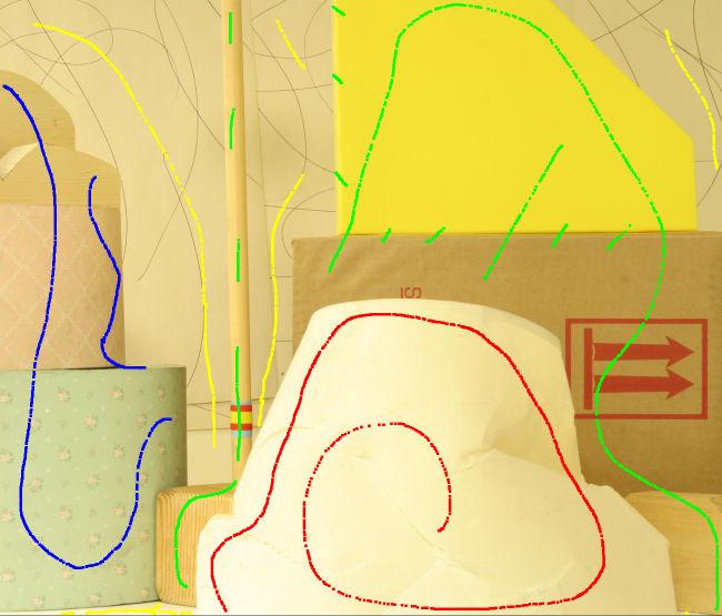
88 Input images and scribbles Estimated Depth Our results Lampshade 2 Midd 1 Baby 1 Legos Tsukuba Figure 5.6: Light-field segmentation results on real datasets from [24, 104]. 83

89 84

90 Chapter 6 Super-rays for Efficient Light Field Processing 6.1 Introduction As we saw on the previous chapter, state of the art light field editing methods either only deal with densely sampled light fields or use a dense depth estimation to perform user-guided segmentation [60, 114] or to propagate user inputs [105, 106, 131, 110, 132]. Despite the latest advances [29, 65, 33, 26] in light field depth estimation, these methods use computationally expensive regularization to obtain satisfactory depth maps. Our goal is instead to propose a solution for unsupervised light field over-segmentation which would in addition be angular sampling agnostic and rely less on depth estimation. Our approach is motivated by the observation that, for most editing applications, it might be more important to have accurate object boundaries, even with coarse depth information, than having a refined depth map. We show in Section 6.4, as already noticed by the authors in [109], that a dense and accurate (in terms of disparity values) depth estimation is not needed for some typical light field applications. To treat the aforementioned problems, we introduce in this chapter the concept of super-ray which is the counterpart of super-pixels [133] for light fields. The major difference with conventional super-pixels and super-voxels is that super-rays group perceptually similar and corresponding pixels across several views. In other words, super-rays are groups of rays of similar color coming from the same scene area. We then propose what we believe to be the first light field over-segmentation algorithm. It is inspired by SLIC [134], a state of the art super-pixel generation method with good properties in terms of accuracy over complexity and parallelism. The major difference is that centroids, initialized on a reference view, are shared by all the views with a unique spatial and color coordinate and an attached depth information. Then, the assignment step is simultaneously performed by projecting the centroids onto each view and the update is done by re-projecting all the rays assigned to the super-ray onto the reference view, using a fronto planar assumption. The approach is fast, free of any strong scene geometry prior, easy to understand and to implement, and it gives satisfactory results. Moreover, it does not require a dense depth map estimation, making it a suitable candidate for a first step of a light field processing pipeline. A new metric is then introduced to evaluate an important feature of super-rays: the view-consistency of the over-segmentation. We also quantitatively and qualitatively test 85

91 our approach on synthetic and real light field data-sets having different angular and spatial resolutions, using standard super-pixel metrics. Finally, in [106, 109] the authors observe that an accurate dense depth map is not crucial for editing. As a follow-up of this work, we show that super-rays enable light field processing tasks which are typically done using a dense depth map, such as light field segmentation and correcting the angular aliasing that occurs when refocusing sparsely sampled light fields. 6.2 Related Work We split the related work in 4 part. First we present the problems with the light field editing methods presented in the previous chapter, then we review existing over-segmentation methods for video, multiview stereo and RGB-D data. Light field editing: In the previous chapter we presented, along with our work, methods that use pixel-level representations [45, 114]. There is one major problem with these works. Unfortunately, global or semi-global regularization methods such as graph cut, do not scale well with the size of the input data, let alone adding a temporal dimension. And although the method we presented in Chap. 5 solves the issue of scalability due to the number of views, views with a too high resolution (e.g. more than 2K) require a very high running time for the graph cut step, which is a problem since the smoothness parameter τ needs to be interactively adjusted. Super-pixel algorithms: Superpixels have been introduced to circumvent this computational complexity issue in traditional image processing. The term super-pixel, first coined in [133] is often described as the partitioning (or clustering) of image pixels into a set of perceptually uniform regions. Ideally super-pixels should be compact (uniform in size), adhere well to the boundaries of objects and be fast to compute. Because of these properties, super-pixels efficiently represent the image content and are often used as an alternative to pixel representations. Super-pixels allow reducing the computational complexity of many image processing tasks such as object segmentation or object tracking, while providing useful region-based information (e.g texture description or guided regularisation). Many super-pixel approaches have been proposed and they can be classified into two main categories (see [135] for a recent overview). The first type of methods concerns graph based approaches [136, 137, 138, 139, 140]. While these methods offer a good accuracy, they either do not provide control on the shape of super-pixels, are very computationally expensive or are not parallelisable, hence not suitable for our applications. The second category of approaches, usually faster than graph-based solutions, aims at growing or evolving existing super-pixels. This category includes a variety of methods such as the multi-scale watershed segmentation approach proposed in [141], the turbopixels segmenting the image into a lattice-like structure of compact regions by dilating seeds [142], and the quick shift clustering technique [143]. In the latter category, one also finds the SLIC [134] and the SEEDS [135] methods for super-pixels on which we focus in the sequel. Simple Linear Iterative Clustering (SLIC) super-pixels [134] rely on a reformulation of Loyd s algorithm for the k-means problem with two novelties. First, the distance metric is a weighted sum of the CIELab color distance and the Euclidean pixel distance. Second a search window around the centroid is used to reduce the complexity of the algorithm. This approach has been extended in [144] to take into account a geodesic distance between pixels. Color and spatial information are integrated along the shortest path between two pixels in order to guarantee compactness, color consistency and connectivity. 86

92 SEEDS super-pixels [135] take quite the opposite approach. The method starts from a regular, coarse grid segmentation, and iteratively updates blocks of pixels at the edge for the current segmentation. That update is done such that each block can change its super-pixel labelling if it decreases a total energy function of the color distribution of the super-pixels. The block size is reduced along the iterations at a given rate. Despite the fact that the last two approaches provide better results, as they enforce continuity between super-pixels, in SLIC, the computation for the assignment and update steps can be done for each pixel independently. This is not the case for all approaches relying on any stack formulation, which makes the methods awkward to implement in parallel. To the best of our knowledge, only SLIC has been successfully implemented on GPUs [145] to provide results in real time. Multiview segmentation: Since a light field can be seen as a (possibly dense) collection of views, the proposed work raises issues one can also find when dealing with multiview segmentation. One issue is in particular the possibility of simultaneously performing segmentation and depth estimation. Super-rays imply establishing correspondences between rays corresponding to different views during the segmentation. The correspondences are found with the help of sparse depth information. While it is possible to simultaneously estimate depth and perform the segmentation [146] or the over-segmentation [147], this can understandably be achieved at the expense of a very high computational cost. As we briefly mentioned in Chap. 5, an alternative approach is to first compute super-pixels independently for each view, and then find correspondences between them. In [118], a graph is constructed connecting relatively small super-pixels computed on each view separately. The super-pixels form the vertexes of the graph, while the edges connect super-pixels in all the neighbouring images that satisfy the epipolar constraint. To enforce spatial consistency, the weights on edges are given by the color-consistency of two connected super-pixels. Using a foreground and background color model, the authors are able to extract a foreground object directly. The goal being object segmentation, the super-pixels are not explicitly grouped in a consistent manner across views, as targeted here with the proposed super-rays. In [148], super-pixels are computed on one view only, and are assigned a normal and depth measure using photo-consistency with the other views. The authors are more interested in estimating depth information in a reference view rather than by the correspondence established by view segments. Video over-segmentation: Over-segmentation has also been studied for reducing the complexity of video analysis tasks. Two main categories of approaches exist for video over-segmentation, either considering a set of consecutive frames as a volume or processing each image separately and updating super-pixels as a new frame arrives. In [149], super-voxels are computed for a set of consecutive frames. The authors assess five super-voxel algorithms in terms of spatio-temporal coherence, object and region boundary detection, region compression and parsimony. Redundancy between frames in the temporal dimension is hence exploited to construct the super-voxels as it is in the inter-view dimension for multiview data. The authors in [150, 151, 152, 153, 154] instead try to compute temporally consistent super-pixels. The approaches hence consist in updating the super-pixels as each frame arrives, either by deleting, creating or updating super-pixels to account for the scene motion. Equally, optical flow is often used as an additional clustering information, but also when large displacements are involved. Although applicable to densely sampled light fields, the first kind of approaches is likely to fail in the case of sparsely sampled light fields as they usually fail for videos in the case of 87

93 large object displacements. The second type of approaches applies to light fields but does not exploit the fact that object displacements from one view to the other is, due to the scene geometry, uniform. RGB-D clustering: To be complete, one should also mention the work focusing on RGB-D over-segmentation. However, this problem differs from ours in the sense that the goal is to segment a point cloud rather than pixels on several views. Nevertheless, one paper [155] interestingly uses a modified version of SLIC, using seeds defined from the 3D map, and performs the assignment step using the image distance from the centroid projection in order to circumvent the errors in depth estimation. Note that this work differs from ours as we do not assume dense depth information to be available and, in addition, we target view segmentation rather than point cloud segmentation. 6.3 Super-ray Light Field Over-Segmentation Let r be a light ray of the light field set L, and (s, t, x, y) its coordinates using the two-planes parametrization as described in the introduction and as in the previous chapter. Each ray also has an associated CIELab color value Lab r. In this chapter, we note (x, y ) := Ps d,t (x, y) R2 the spatial pixel position in view (s, t ) imaging the same scene point, at a distance d, as (x, y) in view (s, t). This is, (x, y) and Ps d,t (x, y) are corresponding pixels imaging the same scene point in different views. In particular, in the case of a uniformly sampled light field we have P d s,t (x, y) = ( d (s s ) + x, d (t t ) + y ). (6.1) However, if the light field has been acquired with a camera array, P should take into account the extrinsic and intrinsic matrices of each camera, and allow us to estimate the pixel correspondences in this particular setting. Using this notation, r r are corresponding rays imaging the same scene point, where r := (s, t, Ps d,t (x, y)). Now, given a light field, our goal is to group in the so-called super-rays, all perceptually similar rays corresponding to the same scene area. Formally, we aim to compute the mapping A: L Z 4 Z, such that each light ray r of the light field is assigned with a super-ray label c. We define S c the set of rays r such that A(r) = c. Each super-ray S c is characterised by a centroid ray r c. By definition, the angular coordinates of r c correspond to the fixed reference view (s c, t c ). Besides, each centroid ray has a depth d c associated to it Method description Initialisation and depth estimation for centroids: First of all, the spatial positions (x c, y c ) of the centroid rays are initialized on a regular grid of step S in the reference view. The corresponding CIELab color values on such positions are the initial color values of the centroid rays Lab rc. Then, a depth d c is estimated for each centroid ray r c. As this step is important for the rest of the algorithm the depth estimation needs to be robust. Thus, inspired by the recent works on light field depth estimation [26], we consider a multi-baseline block-matching strategy with angular patches in order to be more robust to occlusions and fattening errors. Let Ω be the set of angular patches where each patch o Ω is defined such that o(s, t) is 1 if a ray is visible on the view (s, t), and 0 otherwise. Each angular patch can be seen as a 88

94 Figure 6.1: Example of angular patches in Ω for a light field of 3 3 views. The orange color corresponds to the reference view (s c, t c ) so the angular patches are equal to 1 at this position. White positions corresponds to visible rays, so its value is equal to 1, and grey positions are equal to 0. The leftmost patch assumes the ray is visible in all views. Other patches correspond to partial visibility. visibility mask. In practice, we define Ω as a predefined set of angular patches, one patch that corresponds to the full view visibility and eight patches corresponding to different half view visibilities (top-bottom, right-left and diagonals). See an example for a 3 3 light field in Fig Hence, the depth for the centroid c is estimated, given a range of depth candidates D, by minimizing the color distance in the RGB color space using the different angular patches : { } d c = arg min min o(s, t ) Δ B RGB(r c, r c), d D o Ω s,t where r c = (s, t, Ps d,t (x c, y c )) and Δ B RGB(r c, r c) ( = RGBrc (i, j) RGB r (i, j)) 2 c, (i,j) [ B,B] 2 (6.2) is the patch color distance between the patch in the reference view (s c, t c ) and the patch in (s, t ) (s c, t c ). In particular, RGB rc (i, j) = L(s c, t c, x c + i, y c + j) is the RGB-color value of the ray (s c, t c, x c + i, y c + j). In this work, we fix B = 3 and we consider 9 angular patches (their size being equal to the number of views in the light field). Since the depth is estimated for a few points (the centroids), this choice is acceptable for low complexity applications. Assignment step: At each iteration, each light ray r(s, t, x, y) of the light field is assigned a super-ray label. First, the depth estimation in the previous step is used to compute the corresponding rays of r c. Formally, we compute r c = (s, t, P dc s,t (x c, y c )) such that r c r c. Then, each ray in a neighbourhood N S (r c) of size S around r c, is assigned to the super-ray S c if it minimizes the color and spatial distances: ( ) A(r) = arg min Δ Lab (r, r c ) + m Δ xy (r, r c), c where Δ Lab (r, r c ) = Lab r Lab rc 2, Δ xy (r, r c) = (x, y) P dc s,t (x c, y c ) 2, (6.3) and m is the parameter weighting the color and spatial distances. A visual explanation can be found in Fig 6.2. Note that, when r belongs to the reference view, r c = r c in Eq. 6.3 and our assignment step is equivalent to the SLIC assignment step. However, our approach allows to coherently assign a label to all rays in the other light field views. In our assignment step we assume, as in Chap. 5, that two light rays from the same view and close spatial coordinates are likely to image two close scene points. Therefore, a ray that is similar in appearance and close to a centroid light ray or close to one of its corresponding rays is considered likely to belong to the same scene object. Therefore, it should belong to the super-ray corresponding to this centroid. Update step: In this step, the spatial coordinates of the ray centroid and its corresponding Lab values are updated. In particular, the new color value of r c is the average of the color 89

95 r S (x, y) Δ P dc s i,t i (x c, y c ) r c (s i, t i ) (x c, y c ) P dc s j,t j (x c, y c ) (s c, t c ) (s j, t j ) Figure 6.2: The assignment step. r is a ray inside the search window of the super-ray S c, defined according to the projection of its centroid r c, P dc s,t (x c, y c ) in the view where r lies. The color and spatial distances in Eq. 6.3 is denoted Δ. values of all rays in S c and the new spatial coordinates are the average coordinates of all light rays, r = (s, t, x, y) in S c projected on the reference view using the depth d c : Lab rc = 1 S c (x c, y c ) = 1 S c Lab r, (6.4) r S c s c,t c (x, y). (6.5) r S c P dc Note that the centroid rays are defined on a reference view so its angular coordinates (s c, t c ) are not changed in our algorithm. On the contrary, the centroid spatial coordinates (x c, y c ) are first initialized on a regular grid in Z 2 and then updated in Eq. 6.5, which produces new coordinate values in R 2. So, r c is defined as a virtual light ray which is not necessarily one of the light rays captured in the light field. We summarize the update step in Fig When updating the spatial coordinates we assume that rays inside the same super-rays are likely to have similar depth, so Eq. 6.5 is a good approximation with respect to the centroid position we would obtain using the true depth per ray. Furthermore, Eq. 6.5 ensures that two corresponding rays, on two different views, have nearly the same spatial distance Δ xy (as in Eq. 6.3) from a given centroid ray. This is not necessarily the case when seeding the centroids independently on all the views. Cleanup step: Similarly to SLIC, our algorithm does not enforce super-ray spatial connectivity, so after our light ray grouping procedure some rays may remain isolated, specially when the spatial term in Eq. 6.3 has a low weight. For this reason, a simple postprocessing is performed, that consists in re-labeling super-ray disconnected components (with a number of pixels < 1 4 S2 ) with the closest super-ray label. The entire algorithm proposed in this chapter is described in Algorithm 1. 90

96 (x i, y i ) (s i, t i ) P dc s c,t c (x i, y i ) (x c, y c ) P dc s c,t c (x j, y j ) (x j, y j ) (s c, t c ) (s j, t j ) Figure 6.3: Update step. Each ray of the super-ray S c is reprojected on the reference view using the depth of the super-ray. Here we show r i and r j being reprojected on the reference view (s c, t c ). The projections are averaged, giving the new centroid ray position on the reference view (x c, y c ) Experiments In order to quantitatively evaluate the proposed approach, well-known super-pixel quality measures can be trivially extended considering all views, such as the Achievable Segmentation Accuracy (ASA), the Boundary Recall (BR) [156] or the Corrected Under-segmentation Error (CUE) [135]. However, these measures do not evaluate the coherence through the light field views. For this reason, we introduce a new evaluation measure called View Consistency (VC). This new measure assumes that the ground truth depth d r is known for each ray r and uses it to select the light rays to consider. Indeed, given a light ray r, our measure aims at evaluating the assignment consistency for the set of corresponding rays imaging the same scene point as r: L r = { r L s.t. (x, y ) = P dr s,t (x, y), (x, y) = P d } r s,t (x, y ), (s, t ) (s, t). (6.6) Note that the re-projection check using the ground truth d takes into account the occlusions and guarantees that L r contains light rays imaging the same scene point. Therefore, we define V C(A) = 1 1 L L r L r r L r δ A(r) A(r ), (6.7) where δ is the Kronecker delta. This metric is somehow related to the Inter-Frame Label Consistency [151] for super-pixel evaluation in the case of videos, but instead of computing the consistency from frame to frame using the ground truth optical-flow, we measure the consistency between all light field views simultaneously using the ground truth depth. Our quantitative evaluation is performed on synthetic datasets, with segmentation and depth ground truth. We use the dataset in [34], that is composed of 9 9 densely sampled 91

97 Algorithm 1: Super-ray algorithm Data: Input Light Field L Result: Super-ray assignments A Initialize centroids on reference view; while not (converged OR max. iteration reached) do \\ Assignment step for each centroid c do for each view (s, t ) do Compute (x c, y c) = P dc s,t (x c, y c ); for each ray r in N S (r c) do A(r) = c (c minimizing Eq. 6.3); \\ Update step for each centroid c do Compute Ps dc c,t c (x, y), r S c ; Update Lab c and (x c, y c ) (Eqs. 6.4 & 6.5); Cleanup step views of pixels (Papillon 2, Horses 2, Stilllife 2, Budha). We also use the dataset in 5, which is a 4 4 sparsely sampled light field views of pixels (Scene 4). Finally, we propose a new dataset of 5 5 views of pixels (Tricycle), which is rather sparse. First, we observe that our approach converges in iterations, similarly to SLIC, as shown in Fig. 6.4, for both dense and sparse light fields. We compare the proposed super-rays construction method with what we would obtain by separately computing super-pixels on each view, and then merging super-pixels having the highest number of corresponding rays across views. In particular, we use the ground truth depth in the synthetic datasets to re-project rays onto the central view, and we then merge the super-pixels of different views with the super-pixels on the central view having the highest number of re-projected rays, i.e such that V C is maximised. Fig. 6.5 and Fig. 6.6 show the superiority of our strategy compared to the merging of independent super-rays. Fig. 6.5 shows the behaviour of the four quality metrics (ASA, BR, CUE, VC), when varying the different parameters, i.e., the size S of the super-rays and the compactness parameter m, for the dataset Scene 4. We observe in Fig. 6.5a that when increasing the values of S and m, the super-rays do not segment correctly the objects in the scene, as it was observed with SLIC super-pixels. We also remark that ASA, BR and CUE have similar behaviours with similar numerical values when varying S and m, but the proposed metric VC has an opposite behaviour. Indeed, decreasing S and m decreases the view consistency. This can be explained by the fact that decreasing S and m increases the number of super-rays, hence of super-ray edges near which rays are more prone to labelling errors. So, the view consistency decreases. Fig. 6.5b shows that merging independent super-pixels has no impact on the super-pixel metrics (ASA, BR, CUE) as one may expect, but view consistency is severely deteriorated. The same observations generalises to the rest of our test set. Fig. 6.6 shows how the two approaches compare when fixing one of the parameters. To be able to compare light fields of different spatial resolutions, we use k, the number of visible super-rays per view. Once again, we observe very close results when changing k and the spatial weighting 92

98 Average displacement Papillon 2 Horses 2 Stilllife 2 Budha Scene 4 Tricycle Iterations Figure 6.4: Average displacement in pixels of the centroid spatial coordinates with respect to the number of iterations. parameter m for the ASA, BR and CUE. However, enforcing the super-rays to have the same centroid ray imaging the same scene point, yields super-pixel consistency across views. Our approach allows the segmentation consistency to be independent of the parameters k and m, whereas when computing super-pixels on each view, one super-pixel on a view can be described at two (or more) disjoint pieces of super-pixels on another view, depending mostly on the initial seeding. The other thing we notice is the significant difference in terms of over-segmentation performance between densely sampled and sparsely sampled light fields. The over-segmentation of sparsely sampled light fields is less consistent across views, and usually slightly less accurate than for dense light fields. This can be explained by errors in the initial depth estimation, leading to some inconsistent super-rays. Fig. 6.7 and 6.8 show the super-rays constructed by the proposed algorithm, with m = 1 for the smoothness parameter and S = 15 and S = 20 for the super-pixels size respectively. Note that we only display 3 3 views for the sake of readability. Each super-ray is reassigned a random color, the projection of each centroid ray on the different views is represented with a small cross. At a first glance, the super-rays on each view look like regular super-pixels, but the main difference is that super-rays are overall consistent from a view to another, despite occlusions. We invite the reader to zoom in to see the details. Regarding the running time, we currently have two implementations, one on CPU using C++ and the other one on GPU using Python and Opencl. None of these implementation is optimised (the GPU implementation uses global memory and atomic operations) but still give low run-time on our laptop equipped with an Intel i7 5600U and a Radeon R7 M260X. On the Tsukuba dataset, the super-pixels are computed in 6s and 0.3s on GPU. For the dataset of [34], we have a run-time of 80s on CPU and 4.2s on GPU 1. For Lytro Illum light field, it takes 57s on CPU and 3s on GPU. We invite the reader to consult our website 2 for more detailed results. 1 we used 7x7 views on GPU because the entire light field overflowed the maximum allowed buffer size in our implementation

99 1 1 ASA m S BR m S CUE m 100 S VC m 100 S (a) Super-rays evaluation ASA m S BR m S CUE m S VC m S (b) Evaluation of independent super-pixel estimation and a posteriori merging. Figure 6.5: Different evaluation metrics across different parameters for Scene 4. Green means good score while red represent bad score. For the sake of readability, the axes are flipped differently for each metric. 94

100 ASA 0.8 ASA ,000 1,500 2,000 k m BR 0.5 BR ,000 1,500 2,000 k m 0.15 CUE CUE ,000 1,500 2,000 k m 1 1 VC 0.8 VC ,000 1,500 2,000 k m Papillon 2 super-rays Stilllife 2 super-rays Scene 4 super-rays Papillon 2 independent super-pixels Stilllife 2 independent super-pixels Scene 4 independent super-pixels Horses 2 super-rays Budha super-rays Tricycle super-rays Horses 2 independent super-pixels Budha independent super-pixels Tricycle independent super-pixels Figure 6.6: Comparison of super-rays versus merged independent super-pixels, when varying k, the number of super-rays visible on each view with m = 1 fixed (left column) and when varying m the compactness parameter, with k = 500 fixed (right column). 95

101 (a) Original light field (b) Color-coded super-rays Figure 6.7: Super-rays for the sparsely sampled light field in the Tsukuba dataset [24]. (a) Original light field (b) Color-coded super-rays Figure 6.8: Super-rays for the densely sampled light field we have captured with the Lytro Illum and decoded using the toolbox in [47, 157] Discussion The main interest of super-rays is to give a compact mutli-view representation of the scene, without relying on dense depth estimation. This representation can be used directly or with depth information associated to each centroid ray, as we show in the next section. One main challenge of super-rays is to be as computationally efficient as super-pixels. While it would be possible to integrate some photo-consistency prior in the assignment step (Eq. 6.3), this would come with a huge computational cost, since the photo-consistency would either need to be pre-computed for each ray and for each candidate disparity value, or to be computed at each iteration. Moreover, the K-means strategy applied here relies on some strong assumptions on the data (e.g. spherical distribution variance or uniform cluster size), that get easily violated when dealing with other quantities such as color and spatial information. Instead, our approach only uses the disparity of centroid rays, and lets the spatial distance of the re-projected rays do the grouping. In that sense, the geometric information given by the light field is not fully exploited, but on the other hand, as long as two objects have sufficiently different colors, our approach is still sufficient to yield a good segmentation. The first obvious limitation of this method is that it relies heavily on the centroid depth initialisation. Even if we propose a method to robustify this initial search, errors may have negative consequences on the output segmentation, rays being assigned to the wrong super-ray. Precisely, this is a problem when the disparity error is greater than the super-ray 96

102 size, as the centroid would potentially fall outside an object during projection. This being said, light-field depth estimation is an active research topic and our depth estimator could be replaced in the future with another sparse and more accurate method. The second limitation is related to occlusions. Indeed, because the projected centroids coordinates are not placed regularly, but rather warped according to the scene depth, zones with large occlusion have few, or no nearby centroids projections. If an occlusion is bigger than the search window of the super-ray, rays of a view might not be assigned to any super-rays. 6.4 Super-ray Applications In this section we propose two examples of editing applications that exploit the super-rays presented in this chapter. On the one hand, we present a fast light field segmentation algorithm based on super-rays. On the other hand, we present a novel algorithm for correcting angular aliasing for sparsely sampled light fields Real Time Interactive Segmentation Light field segmentation has a high computational complexity [60, 114] and using superrays is a good strategy for decreasing it, similarly to temporal super-pixels for video segmentation. We use the same graph structure introduced in Chap. 5, only this time we do not need dense depth maps. We use the super-rays and the centroid depth estimates to create the graph. This is, we build a graph G = {V, E} where each node in V corresponds to one super-ray S c and we set an edge in E between two nodes if the two super-rays share a common border in at least one view (adjacent super-rays). This decreases the number of nodes approximately by the size of a super ray, giving a graph of hundreds to few thousands of nodes instead of millions. Then, we define the energy ϕ Ω = c i U(c i ) + τ P(c i, c j ), (6.8) c i c j N (c i ) where as before τ is the smoothness parameter, U and P the unary and pairwise terms respectively. N (c i ) is the set of super-rays that are adjacent to c i. U uses the superray average color probability, defined as in Chap. 5 from a Gaussian mixture learned from the user input and P is defined as a summation of the view conventional pairwise relationship. In order to minimize Eq. 6.8 the multi-label Graph-Cuts algorithm in [101, 122] is also applied, using the same available implementation 3. Fig. 6.9 shows the final segmentation for the Tsukuba dataset along with the input scribbles in the reference view and the results of Chap. 5 for comparison. The main interest of using super-rays as a base for segmentation is the gain in running time as summarized in Tab.6.1. For the Tsukuba data set, the graph cut applied on super-rays only takes 1 ms on the same machine as in Sec (a laptop with an Intel i7 5600U and a Radeon R7 M260X). The complete segmentation algorithm takes 8.1s on CPU with the following running times for each step: 6s to compute the super-rays, 2.1s to build the graph (i.e to compute the models, unary and pairwise costs), 1ms to do the graph cut

103 (a) Reference view with input scribbles (b) Super-rays segmentation (c) Chap. 5 segmentation Figure 6.9: Graph-cut segmentation of the dataset Tsukuba using our super-rays. In (a) we show the reference input view with color-coded user annotations, in (b) and (c) we compare the corresponding segmentation masks obtained when using our super-rays and the techniques of Chap. 5 respectively. Our strategy allows a significant reduction of the running time compared to the state of the art light field segmentation. With super-rays computed on GPU, the segmentation only only takes 2.4s with 0.3s for the super-rays computation, 2.1s to build the graph, and 1ms to do the graph cut. On the dataset in [60] the approach takes 94s (80s for the super-rays, 14s to build the graph, 4ms for the graph cut) on CPU and 18.2s (4.2s for the super-rays, 14s to build the graph, 4ms for the graph cut) on GPU. These running times are significantly reduced compared with the state-of-the-art methods in [60, 114] and our previous chapter. The authors in [60] report a segmentation time between 6 and 10min, including 1 to 5min to learn the models and 5min to perform the optimization on a more powerful desktop GPU (Nvidia GTX 580). The approach in Chap. 5 which uses depth to reduce the number of nodes in the graph takes 9.3s on the Tsukuba dataset with the same hardware. It takes 6.3s to build the graph and 3s to do the segmentation. On the dataset in [60] and using real depth, in contrast to what we indicated, the approach in the previous chapter takes 122.6s (82s to build the graph, 40s to do the segmentation). The above figures for the reference methods in [60] and Chap. 5 do not take into account the time needed to compute the dense depth map on each view, while our super-ray construction method includes the coarse depth estimation. For a fair comparison, the time needed to estimate the dense depth maps should be added to the above timing reported for [60] and Chap. 5 which respectively takes 2.9s and 33.6s for the Tsukuba data set and the data set in [60] using the approach in [73] (implemented as pre-processing on a desktop GPU using C++/OpenCL). 98

104 Table 6.1: Comparison of the total segmentation running times, including depth estimation if any. Results of [60] were computed on a more powerful machine than the others. Dataset Approach Tsukuba [60] dataset [60] (GPU) N/S to 633.6s Chap. 5 (CPU) 12.2s 156.2s Ours (CPU) 8.1s 94s Ours (GPU) 2.4s 14s Table 6.2: Segmentation accuracy (ratio of pixel assigned to the right labels according to the ground truth) with a synthetic dataset. The parameters were fixed to k = 2000 and m = 1. We first show our results with respect to the dominant ground truth label assignment for the segmentation (as when computing the ASA metric). This allows us to measure the loss in segmentation accuracy solely introduced by the super-rays (i.e assuming the segmenting process does not introduce additional errors). We also give the results using the super-rays followed by the graph cut approach of Chap. 5. Dataset: Still life 2 Papillon 2 Horses 2 Budha Result in [60]: Result from Chap. 5: Our results (GT Segmentation) Our results (Graph cut) In conclusion, in the context of interactive segmentation, we see that avoiding to compute dense depth maps and running the segmentation on a much more compact light field representation allow a significant reduction of the segmentation running time on CPU, and thanks to the parallelizable nature of super-rays, a dramatic reduction when using GPU. We are confident that more implementation efforts will lead the super-rays computation to be near real-time. This gain comes at the expense of losing precision, but the obtained accuracy is sufficient for many real-time applications requiring a fast (rather than accurate) segmentation. We illustrate this loss of accuracy in Tab 6.2. We see that super-rays introduce errors with a rate of 0.1% to 2% in the best case scenario, when the algorithm used to assign a label to each super-ray does not do any error. Using the graph structure and the data and pairwise terms introduced in Chap. 5, the accuracy drops, with an error rate of 1% to 3%, mostly due to the limited data cost model. Using a more complex model, using textural information provided by super rays will solve this issue Correcting Angular Aliasing As we previously stated, one of the major new light field applications compared to conventional cameras is the post-capture image refocusing. In fact, light fields captured with plenoptic cameras provide quite impressive refocusing results [17] but angular aliasing appears when refocusing light fields from camera rigs or angularly sparse plenoptic cameras. This is due to the poor angular sampling of such acquisition systems. Angular aliasing is particularly visible when the simple shift-and-add algorithm is used for refocusing, whereas, as we previously saw, other solutions such as the adaptive splatting [48] or the rendering 99

105 of novel views [91, 15] decrease the artifacts. However, these solutions are depth-based methods which makes them unsuitable for fast editing applications. Here we propose to refocus using our super-rays to avoid angular aliasing while maintaining a low complexity. Our goal is not to render new views but our philosophy is similar in the sense that we use approximate intermediate views computed with our super-rays. Thus, refocusing is performed via shift-and-add using both original and approximate intermediate views that we call virtual views. With our notations, the shift-and-add method to compute the refocused image at depth d from the viewpoint (s c, t c ) is defined as Is d c,t c (x, y) = 1 N 2 RGB(s, t, Ps,t(x, d y)), (6.9) s,t where the original angular coordinates s, t = 0,, N 1; correspond to the original image views available in the light field, and in the case of a Lumigraph light field, RGB(s, t, P d s,t(x, y)) = L(s, t, x + d(s c s), y + d(t c t)). Now, we define the virtual positions (u, v) R 2 as (u, v) = (s, t) + 1 ɛ d (i, j), i, j = 1,, ɛ d 1, (6.10) where the number of virtual views between two original views is ɛ d = [ (d c d) ] the integer part of the absolute value of the depth difference between the refocusing depth d and the centroid depth d c, c being the centroid label to which (s c, t c, x, y) belongs. Therefore, the corrected refocused image is defined as the sum of the original images and the virtual views contribution: Î d s c,t c (x, y) = 1 { (N ɛ d ) 2 RGB(s, t, Ps,t(x, d y)) + } RGB(u, v, Pu,v(x, d y)). (6.11) u,v s,t Note that Eq requires to interpolate the virtual views, which can be quite memory and time consuming. However, in our strategy we do not explicitly compute them but we use the super-rays depth d c to approximate ray colors in virtual views: RGB(u, v, P d u,v(x, y)) RGB([u], [v], P dc [u],[v] (Pd u,v(x, y))), (6.12) where ([u], [v]) is the closest original view. Considering d c as the depth of all rays of a super-ray is a coarse approximation but it has few or no consequences on the final result since we only approximate for the blurred, out of focus areas. However, the high frequencies on the blur due to the poor angular sampling are successfully removed. Moreover, using the approximate depth information is sufficient to prevent out of focus rays coming from the background to be mixed with occluding in-focus rays which may create artifacts. Fig shows the angular aliasing correction using the dataset from [24] when refocusing at the sculpture bust. Our method successfully decreases the angular aliasing on the background. Note that we simulate a squared aperture which provides a squared bokeh. Finally, we compare our approach with the two-cnns view synthesis approach [91] we presented in Chap. 4. It provides excellent results, with quite big computational cost both for training but also for generating the views (the authors report 12s to generate a single 100

106 GT 2x2 views GT 8x8 views [91] Super-rays Figure 6.10: Angular aliasing comparison. From left to right, we show the images refocused with the 2x2 corner views in the test set in [91], the full 8x8 light field (ground truth), the 8x8 synthesized light field with the approach in [91] and the 8x8 light field synthesized with our approach. We use k = 1000 and m = x376 view). Their training and test set consist of Lytro Illum light fields. Only the four corner views are kept, giving a sparse light field with a very small number of views, and the 60 views in between these images are generated to extrapolate an 8x8 light field which is compared to the captured Lytro Illum ground truth. We use our approach on the 2x2 corner views to generate the other views the same way. The parameters used were k = 1000 and m = 1. The computation of the super-rays takes 0.36s (0.17s per iteration) and generating a view takes 0.007s. Then, we compare on Fig the refocused image obtained with the shift-and-add algorithm using the 2x2 views, the synthesized views from [91] and our synthesized views using the super-rays. We also show the refocused ground truth using the 8x8 Lytro Illum real views. Quantitatively, on the test set, the average SSIM (Structural Similarity) and PSNR (Peak Signal to Noise Ratio) between the ground truth refocused image and our approach is respectively 0.98 and 39.0 versus 0.99 and 42.6 using [91] and 0.92 and 34.5 for the image refocused using only the 2x2 views. Note that we had to crop a 22 pixels border on the reference and our refocused images to comply with the output of [91] that loses the border pixels. Overall, our results are of lower quality because of depth estimates, but in the zones where depth is correct, we see no or few differences between our result and the ground truth. However, our approach has a significantly lighter complexity compared to [91] (the authors report 10s to generate a single view using Matlab and CuDNN, while our approach 1 runs in the order of 100s) which is the main interest of our super-rays. 101

107 Figure 6.11: Refocusing the sparsely sampled Tsukuba dataset. Left: Shift-and-add algorithm which creates disturbing angular aliasing artifacts. Right: Our strategy using real and virtual views. The virtual views have been rendered with our super-rays. We invite the reader to zoom-in to see the details. 6.5 Conclusion We have introduced the concept of super-ray and we have proposed an implementation that is suitable for sparsely and densely sampled light fields. Our solution is fast, easy to implement, and suitable for GPU implementations. Besides, our super-rays are view consistent, which is a major advantage for light field editing. In particular, we have shown the interest of super-rays for light field segmentation and refocusing without angular aliasing. In the future, the proposed approach could be used for other light field editing tasks, such as intrinsic decomposition [158] or video light field processing. 102

108 Chapter 7 Dynamic Super-Rays for Efficient Light Field Video Processing 7.1 Introduction Not only in this dissertation, but also in the current literature, most of the used light field content was static. This is perhaps due to the difficulties of capturing a dynamic light field for either of the aforementioned devices. Specifically, camera gantries are by design unable to record dynamic light fields, and the available plenoptic cameras are either limited to static light fields (e.g. Lytro cameras) or cannot easily produce a Lumigraph as we saw in Chap. 3. Camera arrays require to build a synchronized camera acquisition system, which is a real technical challenge. However, latest advances in light field video acquisition systems [13, 2] show that it is possible to capture quite voluminous light fields in real time, without specific hardware and with reasonable capturing systems. The problem of efficiently processing the captured 5D light field content is then twofold. First, the amount of data to handle, already a problem for static light fields, reaches a critical point for video light fields. As a consequence, computational efficiency is a core aspect in many light fields processing tasks, such as editing. Secondly, to enable editing via user interaction on a single key frame, algorithms must consistently propagate the edits angularly and temporally to the rest of the dynamic light field. In this last contribution chapter, we build on the work in Chap. 6 to present an oversegmentation scheme that exploits the light field redundancy in both the temporal and angular dimensions and leverages GPU computational power to enable easy and fast light field editing from a single reference view and frame. The proposed over-segmentation approach generalizes the concept of super-rays, to dynamic super-rays for video light fields. Several constraints are taken into consideration in the design of the proposed method. First, the approach is kept parallelizable to take advantage of a GPU implementation. Second, it processes different frames sequentially and on-the-fly, so the memory footprint is reasonable, in contrast to methods operating on sliding windows. This is mandatory as the amount of data per frame is much greater than a conventional 2D video. Finally, super-rays are consistent across views and across frames in the temporal dimension. Specifically, our contributions are: 103

109 An end to end approach to create an angularly and temporally consistent light field over-segmentation that we call dynamic super-rays A new update term for creating and deleting superpixels and super-rays specially tailored for dynamic content A new strategy for creating a temporal over-segmentation that is consistent with the scene movement 7.2 Related Work The related work of Chap. 6 is also valid for this chapter. However, we only briefly mentioned methods that aim to compute a dynamic over-segmentation for conventional, 2D videos. We give more details on how these methods work in this section. The first one assumes the entire video sequence to be processed as a whole. For instance, in [134], the temporal dimension is treated in the same way as the spatial dimensions in order to create a single volume, where volumetric superpixels are computed. Whereas in [159], superpixels are computed separately on each frame, then temporal correspondences between superpixels are established using an affinity metric in order to extract object segments. The second and more popular category aims at computing the segmentation consistently, from a frame to another. Several approaches have been proposed. In [151] a pre-computed dense optical flow is used along with a Gaussian process to update the labeling from a frame to another. The superpixels deletion or creation is done by inference using the same Gaussian process. In [153], the framework proposed in [160] is extended to videos. When a new frame arrives, the same moves are performed to adapt for the new frame geometry, using the previous frame assignments. Creation and deletion of superpixels are done by looking at color histogram distances. In [152], the most related work to ours, dynamic SLIC superpixels are computed in a sliding window of 20 frames. A dense flow is used to propagate the assignment from a frame to another and several SLIC iterations are run. The centroid color is shared between corresponding superpixels on several frames of a sliding window. The superpixel update criteria is solely based on the superpixel size evolution. Unfortunately, none of the aforementioned approaches are readily applicable for video light field over-segmentation for different reasons. Loading all, or a large amount of the frames of the video sequence as in [152, 134] is prohibitive in the case of a light field. Performing a late merge of frames superpixels as in [159] does not provide any temporal consistency. Methods taking the assumption that the temporal dimension is densely sampled, as in the temporal propagation step of [151], will most likely fail in our case, where objects with wide motion are involved. Finally, all the approaches relying on a stack of granular operations as in [153], are not suitable for a GPU implementation, necessary to handle the large volume of data in editing time. 7.3 Dynamic super-rays The proposed approach is a follow up to the previous chapter and is inspired from techniques proposed to generate temporally consistent superpixels [152, 151], that can be decomposed into three main steps: (i) initialize the current frame segmentation by temporally propagating the segmentation of previous frames, (ii) adapt the segmentation to changes in geometry and (iii) create and delete segments to take into account occlusions and objects entering or leaving the scene. 104

110 Frames δ x c Views P d c P d+δ d c Figure 7.1: Illustration of our algorithm in a simple case. The red foreground super-ray is tracked over the consecutive frames of a 2 1 light field. Other super-rays do not move since the background is static. The depth d is used to enforce angular consistency from a view to another, while the scene flow (δ x, δ d ) guarantees temporal consistency. On the third frame, the moving red super-ray becomes too close to the pink super-ray and too far from the green one, triggering the creation of the orange super-ray and the deletion of the pink one on the next frame. In this chapter, we consider a dynamic light field L f with the temporal dimension being denoted by superscript f. We use almost the same notation as in Chap. 6 for the super rays index S c of label c, the assignments A are now temporal assignments A f, dynamic rays are noted r f. We however collapse the angular and spatial coordinates into (s, x) to avoid long equations. P then becomes x := P d s (x). Our algorithm is summarized in Alg. 2 and illustrated in Fig Algorithm 2: Dynamic super-ray algorithm Data: Input light field frame L f Result: Super-ray assignments A f if f == first frame then Compute A f as in Chap. 6 else Move centroids with (δ x c, δ d c ) (Sec ) Delete and create centroids (Sec ) for 5 iterations do Do the assignment step Eq. 6.3 Do the update step (Sec 7.3.3) Sparse temporal propagation Computing a dense and accurate optical flow for light fields can be a quite tedious task, especially when memory and time requirements are taken into account. Moreover, because super-rays embed a depth information per segment, the problem we aim to resolve is a scene flow estimation problem. That is, we aim to find the displacements of 3D points in 105

111 the scene rather than pixels shifts in the image plane. Fortunately, in the case of super-rays, the scene flow estimation needs to be estimated only for centroids and not for all rays of the light field. Formally, for two consecutive light field frames f and f + 1, one could estimate the scene flow (δ x c, δ d c ) at the centroid ray r f c = (s c, x c ) as (δc x, δc d ) = arg min Δ B RGB(rc f+1, r c f+1 ) δ x,δ d s where rc f+1 = (s c, x c + δ x ) and r f+1 c = ( s, P dc+δd s (x c + δ x ) ) ; (7.1) and Δ B RGB r c f+1. the color distance between two patches of size B centered at rf+1 c However, this 3-dimensional cost function being quite expensive to minimize, we have split the problem into optical flow and depth estimation, like other methods for light field scene flow estimation in the literature [28, 161]. Besides, it is not clear to which extent solving jointly the displacement for x and d would be beneficial. Now, in the state of the art optical flow estimation methods [162] Deep Flow [163] stands out for its performance in terms of quality and run-time. Deep flow first searches for sparse matches using Deep Match [164] between downsampled versions of the input frames, and then the matches are densified by regularizing a selected set of sparse matches. Deep Match has many properties which are interesting for our problem. It is robust and efficient since it can be implemented on GPU 1 and the matches are searched in a limited local window. Thus, we solve the sparse flow estimation using deep matches. In contrast to Deep Flow, we do not seek to obtain a dense and precise optical flow, but rather a robust and fast sparse flow for each centroid. We compute a set of deep matches µ [164], with their coordinates in the reference view noted xµ f and xµ, f from two downsampled frames f and f + 1. Then, the estimated flow δµ x = xµ f+1 xµ, f using the deep matches in the full resolution coordinate system, is used to compute the flow of each centroid δc x using a simple and fast bilinear interpolation. Precisely, δc x is the distance-weighted average flow δm x of its 4 nearest matches. Using the notation above, the depth is updated using the same strategy as in Chap. 6: and { δc d } = arg min min o(s ) Δ B RGB(rc f+1, r c f+1 ), (7.2) δ D o Ω s where D is the small range of potential depth movements and Ω is a family of spatio-angular patches Centroid creation and deletion Because of object movements in the scene, the super-ray topology can change in time. For instance, parts of the super-rays can be occluded or disoccluded, or completely appear or disappear due to objects entering or leaving the scene. For this reason, creating and deleting super-rays might be necessary. While the superpixel size or color consistency has been used to determine the creation or deletion in other research works, we propose to leverage the depth information associated to the super-ray to detect occlusions and disocclusions

112 c up S c left c c right c down Figure 7.2: Super-ray neighborhood. Each super-ray is represented by a solid color and its centroid by a black dot. The search area for the left neighbor c left of the red super-ray c is represented by the blue dots, and the final neighborhood connections of c by the black lines. In particular, a new super-ray is candidate to be created at the midpoint of two super-rays when their centroid distance exceeds a given threshold S q. Conversely, a super-ray will be a candidate to be deleted if two super-rays are too close from each other, i.e. their centroid distance is lower than a threshold S/q. In particular, the occluded super-ray (with the smallest disparity or biggest depth) is the candidate for deletion. For the sake of efficiency, and to avoid duplicates, we search the candidate centroids to be deleted or created in a 4-nearest neighborhood, computed as illustrated in Fig Specifically, the approximate neighborhood of a centroid c is defined as N (c) = {c left, c right, c up, c down } where { } c left = arg min yĉ y c s.t. xĉ < x c, yĉ y c < S, (7.3) ĉ and similarly for the other neighbor centroids. Now, in order to maintain the number of super-rays constant, we create the same number of super-rays we delete. If the number of candidates for deletion is smaller (resp. bigger) than the number of candidates for creation, only the centroids with the biggest (resp. smallest) centroid distance are created (resp. deleted). Finally, because objects can move inside or outside of the reference view, the super-rays near the image borders are treated as follows. New super-rays are created in the reference view between the image borders and the closest centroids. For instance, if a centroid c does not have a neighbor c right, a new centroid will be ( xc+m 2, y c ), M being the reference view width. Super-rays that leave the reference view image plane are automatically deleted. Note that the centroid neighborhood can be used for further processing, as it is a convenient way of representing the super-rays structure New frame over-segmentation In the new frame, after defining the set of centroids in the reference view, all the rays of the light field are assigned to a centroid. Similarly to super-rays, the assignment is done using Eq. 6.3 in an iterative process with color and position centroid updates. While the centroid color is updated with the same color average strategy as super-rays, the centroid 107

113 Frames Views Figure 7.3: Dynamic super-rays for 3 frames and 2 views of the dataset Birthday [2]. position update changes for dynamic super-rays. So Eq. 6.5 becomes ( p xc f+1 = Sc f+1 r S f+1 c ) Ps dc c (xr f ) + (1 p)(xc f + δc x ) (7.4) where p is a parameter controlling how much the super-rays are allowed to move from their theoretical position. When p = 1, this step corresponds to the same SLIC iteration as in Eq. 6.5, and when p = 0, the super-ray centroids are not updated at all, providing the best temporal consistency. Newly created centroids (as described in Sec ) are updated using p = 1, allowing them to adapt to scene changes. In [152], 5 SLIC iterations are run, where the centroids are allowed to move freely. As a consequence, superpixels of static objects tend to move since they are affected by the creation, deletion and movements of nearby superpixels. On the contrary, our dynamic super-rays movement is congruous with the objects movement in the scene, providing a more consistent temporal over-segmentation. 7.4 Experiments Currently, two datasets for video light fields captured with camera arrays are available. The Fraunhofer dataset [13], with sequences of 3 3, 3 5 and 4 4 views, a camera resolution of pixels and sequences between 150 and 400 frames. On the other hand, the Technicolor dataset [2] with sequences of 4 4 pseudo-rectified views, a camera resolution of pixels and sequences between 300 and 390 frames. The cameras baseline is quite important for the second dataset. 108

114 Frames Figure 7.4: Over-segmentation comparison with [152] on the reference view over 5 frames. Our dynamic super-rays (second row) are consistent with the scene movement while the superpixels in [152] (third row) move in static regions. As hyper-parameters, fixed for all the datasets, we use a down-sampling factor of 2 and a flow window of 30 pixels for the computation of the deep matches. The δ d search range is limited to 1/10 of the depth search range, given for each dataset. The depth block size is fixed to pixels. The compactness parameter m is fixed to 0.5 and q and p are fixed to 1.9 and 0.4 respectively. We generated 1500 super-rays for the Technicolor dataset and 2000 for the Fraunhofer dataset. These number of super-rays offer a good trade-off between segmentation accuracy and super-ray tolerance to occlusions (as discussed in Chap. 6) for each of the datasets. Our dynamic super-rays are computed in the whole sequences without fragmenting them. Fig. 7.3 shows the output of our algorithm for a small area of the dataset Birthday [2]. For the sake of visualization, results are only shown for two views, the reference view s c = (1, 1) and another view s = (1, 0), and three non-consecutive frames f = 95, 100, 105. For each view, we show the input image with the optical flow only on the reference view (top left), the color-coded assignment (top right), the super-ray average color (bottom left) and finally the super-ray contours (bottom right). Please note that it is hard to evaluate our over-segmentation results on paper due to the reduced number of frames or views we can illustrate compared with the full light-field videos. We strongly encourage the reader to visualize all our results on our web-page 2. The resulting videos show concatenated views with usual visualization methods, namely, the super-ray average color, the color-coded super-ray labels, and the super-ray contours (as in Fig. 7.3). We also visualize the value of the flow for each centroid, as well as the coarse depth of each super-ray, by assigning the super-ray centroid depth to all the rays having the same label. Finally, we show the centroids neighborhood structure in which the deleted or created centroids are differently colored. We compare our method with the algorithm in [152] which is the state of the art for temporaly consistent superpixels on videos. Note that in this experiment we focus on

115 the temporal aspect since we already show in Chap. 6 that computing superpixels on each of the views separately does not guarantee angular consistency. So, here we show our over-segmentation results for the reference view only. Fig. 7.4 shows this comparison on five frames, f = 260, 262, 263, 264, 265. In particular, on the top row, we show the neighborhood structure described in Sec Each centroid appears as a blue dot, and horizontal and vertical neighborhoods are illustrated with cyan and magenta edges respectively. Centroids of deleted super-rays are represented in red, while new super-rays are represented in yellow. The second and third rows correspond to our results and the results of [152] respectively. We observe that the update step in [152] allows the superpixels on the static background to move freely. On the contrary, our super-rays are not moving so the scene movement is consistent with the super-rays movement. We believe this is a major benefit if dynamic super-rays are to be used in further editing tasks. We invite the reader to view the video in the supplementary material where temporal consistency is more visible 2. Besides the qualitative comparison with [152] we have also observed considerable differences in terms of computational complexity. Depending on the datasets, the algorithm in [152] takes several hours and up to one day (using the original implementation) to run for all the frames of a single view video. In our case, the biggest advantage is the GPU friendliness. Indeed, the SLIC-based iterations, the deep flow computation and the super-ray creation and deletion, are highly parallelizable. On the same machine (equipped with an Nvidia GTX 1080 GPU hosted by an Intel Xeon E CPU) our current Python/PyOpenCL implementation gives an average running time for each iteration of 0.157s and to 0.083s (depending on the input size), respectively on [2] and [13]. Further improvements are to be expected by a more optimized implementation. Dynamic super-rays with the neighborhood structure presented in Sec offer a useful representation of the scene captured by the light field videos. Temporal super-rays can be seen as a powerful tool for efficient light-field video editing in which the edits in one reference view of the light-field can be easily propagated to other frames and views. Apart from the angular aliasing correction and the segmentation presented in Chap. 6.3, dynamic super-rays can be used for temporal image interpolation without flickering caused by an inconsistent interpolation. Other examples of temporal super-rays applications include light-field video compression (e.g. adapting the approach in [165]), or light field color transfer (e.g. using the algorithm in [166]). Limitations: We have observed that our approach has some limitations, in particular, when the depth or the flow estimation becomes erroneous, the super-ray consistency is not guaranteed from one view to another. Such failure case is visible in the dataset Newspeaker [13], where a very uniform green background challenges both the depth and flow estimations. When the depth is inconsistent, the centroids are wrongly projected, leading to large areas with no nearby centroid for the rays to be assigned to. The other failure case involves small moving objects, because of our sparse flow computation strategy, the optical flow for small object can be wrongly evaluated to the flow value of its surrounding. This is visible on the dataset Train [2], where centroids struggle to follow the train wagons. In conclusion, even if depth and flow estimation are mature research topics we have observed that challenging datasets may still produce inaccurate estimates. In particular, the images in the two datasets suffer heavily from motion blur, noise and over and under exposition. Furthermore, the dataset in [13] has some large texture-less areas. However, losing consistency in flat areas is not critical. Indeed, if the zone to edit is totally 110

116 uniform, the editing becomes trivial (e.g. using a simple color threshold), dismissing the needs for super-rays in the first place. 7.5 Conclusion We presented an approach to generate angularly and temporally consistent light field video over-segmentations. Our algorithm design allows a GPU implementation, allowing computational performances that are required to cope with the high volume of data. To the best of our knowledge, this is the first approach to deal with the problem of video light field editing. 111

117 112

118 Part IV Closing 113

119 114

120 Chapter 8 General Conclusion 8.1 Summary Light field imaging is a renewed and dynamic research field. Because of the technical challenges of its capture, the complexity and the trade-off it introduces, a lot of problems remain to be addressed before we see a mass adoption of light fields into conventional imaging pipeline. In particular, we believe that both future phones and professional camera systems could benefit greatly from the geometric information a light field captures, may it be to directly produce better images (e.g. via synthetic aperture, object dis-occlusion, super-resolution) or to provide with a depth-augmented user experience (e.g. view synthesis, depth estimation). In this thesis we addressed two main topics. The first one focuses on image rendering in cases that are somewhat less explored in the literature. Focused plenoptic camera, have the advantage to control the trade-off between the angular and spatial resolution. However, since they are unable to render a Lumigraph without a depth estimation, a lot of the state of the art methods in plenoptic image rendering are irrelevant. In Chap. 3, we proposed a novel end-to-end pipeline to transform a light field captured with a focused plenoptic camera into conventional images. We proposed a calibration that has the advantage of being carried out entirely in the Fourier domain, making it robust to noise and relatively exempt of a particular calibration setup. A novel depth estimation algorithm that uses and combines conventional stereo methods is then used to render all in focus and refocused images, based on splatting approaches, of quality comparable with the state of the art and commercial solutions. Plenoptic cameras trade spatial resolution for angular resolution. An alternative to this trade-off could be to capture only a sparse set of angular samples and reconstruct the rest. In Chap. 4, we investigate a new way of generating intermediate views from a set of only four views. The main goal of the approach is to enable view synthesis on memory and computationally limited devices, and for input images with an arbitrary baseline. We proposed a new usage of recurrent neural networks, and in particular long short-term memory cells to directly learn to synthesize a new view from a plane sweep volume. Our experiments show that, on a limited scenario, our approach does provide good interpolation results. However, our study also shows that in its current state the methods need improvement to handle arbitrary baseline sequences and we give possible direction for further work. In a second part, we addressed the problem of light field editing by methods that compute 115

121 meaningful segments directly in the set of all views of a light field. This is of a particular interest when we need to perform an operation consistently from a view to another, e.g. to remove or to recolor an object from a light field. In Chap. 5, we proposed a novel user-guided and pixel-wise segmentation technique. The goal is, from only one reference view and a set of sparse user annotations, to extract corresponding object segments. Our approach is based on graph-cut, with a graph structure tailored to handle the important number of rays of the light field. Specifically, we leverage a dense depth information to collapse the segmentation graph, decreasing greatly the running time of the segmentation. We also show how the segments can be used for dis-occlusion. Although the results on synthetic data showed to be competitive compared to the state of the art, our approach does rely on a decent depth estimation. Also, as for a lot of segmentation approaches in the state of the art, our method does not scale well with the size of individual views, let alone video light fields. Hence, in Chap. 6, we propose another approach which is more tailored toward realtime automatic editing. We propose an over-segmentation scheme that leverages GPU computational power and that does not rely on a dense depth estimation. The main idea of the approach is to alter the SLIC algorithm (based on Loyd s algorithms for k-means) with cluster centroids that have their average color and spatial positions shared in between views. The obtained segments are then used to interactively segment objects in real-time, and to correct angular aliasing that occurs during synthetic aperture rendering. Because the approach is efficient and scalable, we extend it in Chap. 7 to video light fields. The idea is to propagate temporally the segments in an on-line fashion. Specifically, we use a sparse optical flow on only one view to establish centroid moves and re-run several iterations of the segmentation in Chap. 6 with several variations. First the centroid are forced to only move slightly in order to encourage over-segmentation consistency from a frame to another. Second, centroids are created and deleted using their respective distance as a proxy. 8.2 Future work and Perspectives We believe that the work in this thesis has opened up some interesting research directions. Regarding the proposed plenoptic camera pipeline, the major upgrade to be done in the depth estimation part could be to perform the disparity estimation and the depthtriangulation step at once instead of separately. This especially could help in cases where the disparity algorithm fails. Another improvement could be to leverage the fact that we are in fact refocusing with a known half-aperture mask. Deconvolution methods could be combined with the stereo estimation to extract the depth, similarly to coded aperture approaches. The rendering could also benefit from more advanced techniques than splatting. Global or semi-global regularization could be used to improve the result where the depth is faulty. For view synthesis, we mentioned several ways to improve the methods that need to be tested to definitively validate the use of the proposed architecture. May the proposal of using deeper gates, or use an inferred depth followed by a manual warping, not be enough to provide with arbitrary view synthesis on any baseline, the following re-work of the approach could be proposed. Instead of trying to solve the problem with a single RNN, we could imagine using first a cascade of CNNs with shared weights, taking into input slices of a sparse PSV. The disparity step of the PSV would be inferior or equal to the CNNs receptive fields. The output of each CNN would be a partial disparity map, i.e. a depth 116

122 that is only valid for the areas that are close to their true depth plane on the PSV slice, along with a confidence map, illustrating how confident the network is that the zone is valid. This would be enforced with a loss term, encouraging the warping of the corner views with the partial depth map to be close to the ground truth, if they have a high confidence value (e.g. with a weighted L1 norm). The RNN would then only be taking as input the partial depth maps, along with their confidence to synthesize the final, complete, depth map, along with interpolation weights as in [89]. This proposal, while being significantly heavier than the proposed approach, do preserve the baseline-agnostic part the proposed LSTM method, while delegating the most complicated task (i.e. computing a depth) to CNNs. Augmenting or diminishing the disparity range would be done by simply adding or removing more CNNs with shared weights and adjusting the number of cells in the RNN accordingly. Very recent advances in deep learning allow to use convolutional networks directly on point clouds [167]. An ambitious modification of our graph segmentation method could be to learn an end-to-end automatic segmentation method using a first CNN to compute depth maps and generate the aggregated graph structure, and a second network to do the segmentation on it. Regarding over-segmentation, we took SLIC as our baseline implementation but many new variations for this algorithm have been proposed to improve the overall over-segmentation accuracy. Specifically, if we wish to keep the GPU efficiency part of the approach, a good upgrade could be to use a variant of SCALP[168], that augment the SLIC distance metric with a linear path. It is a nice way to include edge and structure information into SLIC while keeping its low complicity. To end this thesis on a more general note, light fields capturing devices currently have significant trade-offs in terms of quality or computational requirements. However, with the developments of phones, dual and quad pixels sensors, we expect these concessions to be overcome. Light field imaging has been a long-standing research area, and we are excited to see if this progress will finally lead to mass adoption of light field capable devices. We also hope the solutions proposed in this thesis to be useful to provide users with new and interesting imaging capabilities. 117

123 118

124 Appendix A Author s publications This thesis manuscript is based upon the following publications. Articles Conference papers M. Hog, N. Sabater, C. Guillemot, Light Field Segmentation Using a Ray-Based Graph Structure, European Conference on Computer Vision (ECCV), pp , M. Hog, N. Sabater, C. Guillemot, Dynamic Super-Rays for Efficient Light Field Video Processing, British Machine Vision Conference (BMVC), pp. 1 12, 2018 M. Hog, N. Sabater, C. Guillemot, Long Short Term Memory Networks for Light Field View Synthesis, Submitted, 2019 Journal papers M. Hog, N. Sabater, B. Vandame, V. Drazic, An Image Rendering Pipeline for Focused Plenoptic Cameras, IEEE Transactions on Computational Imaging (TCI), vol. 3, no. 4, pp , M. Hog, N. Sabater, C. Guillemot, Super-rays for Efficient Light Field Processing, IEEE Journal of Selected Topics in Signal Processing (J-STSP),

125 120

126 Appendix B List of Notations We use a set of unique and consistent notations for the items that are commons and consistent in between chapters. However, for a sake on simplicity, we might use redundant notations with different meaning in each chapter. Global notations: s, t angular coordinates with the two plane parametrisation x, y spatial coordinates with the two plane parametrisation r an arbitrary ray L the light-field function that maps rays coordinates to radiance We usually consider the radiance to be expressed as RGB or Lab triplets. L light field set of all rays I a Image refocused using a. a can be an arbitrary focus plane or correspond to a particular depth Î a virtual view d depth or disparity D a range of depth or disparity i, j usually denote an arbitrary index value f time coordinate we usually consider a frame index d a depth or disparity θ, ρ a set of polar coordinates N neighborhood of a given item G a graph V a set of graph vertices E a set of graph edges U Unary energy term P Pairwise energy term ϕ Ω energy function for the label assignment Ω τ smoothness parameter used in graph cut usually denotes a coordinate after projection Lab a color in the CIELAB color space of a a can be a ray, a ray bundle or a super-ray c super-ray index S c super ray of index c centroid ray r c 121

127 Chap 2 R the radiance of a ray X, Y, Z 3D coordinates λ ray wavelength Π the plenoptic function A a set of view coordinates defining the aperture of a refocused image Chap 3 microlens diameter T x, T y microlens array offset form the sensor T shortcut for (T x, T y ) α microlens array angle with respect to the sensor k, l pixel coordinate on the raw plenoptic image k, l pixel projection from the sensor plane to rendered image plane m, n pixel coordinate on the rendered image I Raw light field image I w a raw white plenoptic image I a an all-in-focus image I g l, Ig r images refocused at g using the left and right microlens images N size of the image g focal value o k, o l microlens image center Λ line along which the cosine oscillates F m, F p Fourier magnitude and phase ξ peaks coordinate in the Fourier space Δξ a small offset in the Fourier space Γ gamma correction factor V Gaussian noise variance K static splatting kernel λ parameter that controls the spread of the splatting kernel K d g disparity of a pixel between I g l and Ir g g f g value for which a pixel is in focus Δ distance between two pixel in the raw light field K, K adaptive splatting kernel σ image rendering size factor S masking kernel to handle occlusions during splatting Chap 4 I t C t h t σ i σ u σ o Tanh u I d a cell input at step t a cell memory state at step t a cell output at step t the input gate the update gate the output gate the update layer the four input views warped with d 122

128 Î d δ d the synthetic view sat step d a disparity step Chap 5 b R B Ω ω P σ Lab, σ d S ray bundle, i.e. a set of ray coming form the same scene point set of free rays superset of all ray bundles The labelling function that maps labels to pixels An object label notation for conditional probability local variance for the color and the depth Scribbles images Chap 6 k number of super rays x, y projected pixel coordinates P projection function r corresponding ray or r, of coordinates x t s t s c, t c, x c, y c centroid ray coordinates A super-ray label assignments o angular masks B size of a patch Δ B RGB color difference for a patch of size (2B + 1) 2 m weighting parameter between color and spatial distance S max size of a super-ray L r set of all rays imaging the same scene point as r u, v virtual view index Chap 7 Sc f dynamic super ray at frame f δc x, δc y flow for centroid c rc f centroid ray at frame f A f assignments at time f s, x collapsed notation for s, t, x, y µ a deep match xµ f coordinate of a deep match at frame f δµ x sparse flow from deep matches c left/right/up/down centroid neighborhood of c in each cardinal direction m parameter for Lab xy weighting p parameter controlling the centroid temporal moves q threshold update 123

129 124

130 Appendix C Additional Results for Chap 3 Fig. C.1 reproduces the same experiment as with the Donkey test set but with a more challenging close-up setup. The depth estimation on the Lion background is noisy due to the lack of texture in the background. On the Tiger however, there is enough texture to successfully reconstruct the entire depth from the two slices of the focal stack. Fig. C.3 compares the depth we obtain with the depth in [18] and [42] for the images Jeff and Fontain. Finally, Fig. C.2 shows how our algorithms perform for the other images of the Georgiev s dataset. Fig. C.4 show the rest of the all in focus images from the Raytrix R1 dataset we rendered with our pipeline. Interestingly, the images do not present the same artifacts. Ours tend to have sharper edges with less artifact and a better rendering of small textured details. However, our approach struggles with thin structures and areas too close to the camera. Tigre Lion Figure C.1: Depths maps for the other images of our R5 dataset. 125

131 Bike Seagull Laura Fredo Reference Image Our depth map Figure C.2: Our depth maps for the rest of the Georgiev s dataset 126

132 Fontain Photographer Reference image [18] / [42] Ours Figure C.3: Comparison with depth from [18] and [42] (1 depth per microlens) Figure C.4: Our rendered images for the rest of the Raytrix R11 dataset. 127