Radiance Photography. Todor Georgiev Adobe Systems. Andrew Lumsdaine Indiana University

Size: px

Start display at page:

Download "Radiance Photography. Todor Georgiev Adobe Systems. Andrew Lumsdaine Indiana University"

Darcy Barrett
6 years ago
Views:

1 Radiance Photography Todor Georgiev Adobe Systems Andrew Lumsdaine Indiana University

2 Course Goals Overview of radiance (aka lightfield) photography Mathematical treatment of theory and computation Hands on Mathematics Computation Radiance cameras

3 Outline 1. Background, Motivation, and History 2. Radiance Theory in Spatial and Frequency Domains 3. Capturing Radiance with Radiance Cameras 4. Hands-On with Radiance Cameras 5. Computational Methods for Radiance 6. Fourier Slice Refocusing 7. Vario-Plenoptic Camera (Plenoptic 2.0) 8. Wrap-Up

4 Background and Motivation

5 Brief History of Photography

6 Along Came Photoshop Good News: Anyone can edit pictures Bad News: Anyone can edit pictures

7 Photographs are Collections of Pixels Pixel-based manipulation can change presentation of picture But the relationship of pixels to each other (based on scene) is lost Is a given pixel part of the same object? Is it at the same depth as another pixel?

8 Some Enhancements Are Practically Impossible Changing focus Change aperture / depth of field / F/# Changing view point Detect depth Insert objects These depend on how pixels are created Based on scene physics These changes require taking a different picture

9 Radiance (aka Lightfield) Photography A picture is a rendering of the light rays in a scene Determined by lenses, spacing, aperture, etc Record the light itself rather than rendering the light Defer rendering Then we can synthesize any picture we want Not a new idea (over 100 years old) Technology exists now to make radiance photography practical

10 Capturing Light Itself In a traditional photograph, the sensor integrates rays from every direction at each pixel

11 Capturing Light Itself To create an imprint of light itself, at each pixel we capture rays from different directions individually

12 Capturing All of the Light E.g., Stanford camera array 100 custom cameras

13 Practical Radiance Capture We can capture all of the light in front of a camera (or in the camera) Change focus Change aperture Change viewpoint (limited by camera lens size)

14 Rodin Radiance Capture

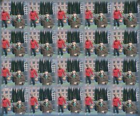
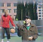
15 Change Viewpoint

16 Change Focus

17 Change Focus

18 Change Aperture / All-In-Focus

19 Brief History of Radiance Photography Since 1903

20 F. Ives Patented 1903 Array of pinholes at image plane

21 Lippmann (1908)

22 Lippmann (1908) Nobel Prize for Color Photography

23 Lippmann (1908) First Described Light-Field Capturing Device

Light-Field Film (1908) See the original paper: http://www.tgeorgiev.

24 Light-Field Film (1908) See the original paper:

25 H. Ives (1930) Lenticular Lens

26 Coffey F/Number Matching (1935)

27 Chutjian (1968) First Digital Light-Field

28 Dudnikov

29 Adelson (1991) Plenoptic Function

30 Adelson (1992) Plenoptic Camera Designed to solve computer vision problems

31 Levoy/Hanrahan (1996) the term Light Field

32 Isaksen (2000) Light-Field Refocusing

33 Ng, Tech Report (2005)

34 Fife (2008) Light-Field CCD

35 Radiance Theory and Modeling The main laws of optics and radiance transforms

36 Radiance Capturing rays from different directions individually Parameterizations: Two plane and Location-angle

37 Two Parameterizations of Rays Two plane Location-angle st uv x

38 Radiance Energy density in 4D ray-space Energy in all small p-cones (each one from p to p ) in a small q-box ( from q to q ), perpendicular to p Energy in a small 4D cube around (q, p), divided by the volume Intuitively it is the light-field or light itself Express radiance as r(q,p)

39 Light Transport Through Space Ray transformation

40 Lens Transform (Ray Bender) The further away from center, the more it bends.

41 Summary Two primary optical transforms are Lens and Transport Lens Transport

42 Composition of Optical Elements Transformations corresponding to compositions of optical elements are determined by the constituent transformations

43 Composition of Optical Elements Transformations corresponding to compositions of optical elements are determined by the constituent transformations What is in terms of

44 Composition of Optical Elements Transformations corresponding to compositions of optical elements are determined by the constituent transformations What is in terms of

45 Composition of Optical Elements Transformations corresponding to compositions of optical elements are determined by the constituent transformations What is in terms of

46 Composition of Optical Elements Transformations corresponding to compositions of optical elements are determined by the constituent transformations What is in terms of

47 In Class Exercise Three lens system Composition:

48 Traditional Camera Transfer matrix:

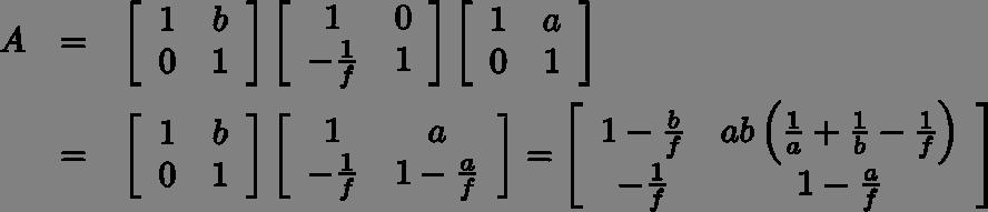
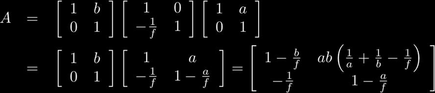
49 Traditional Camera

50 In Class Exercise What is det(a)? Answer: det(a) = 1

51 In Class Exercise How do we focus?

52 In Class Exercise How do we focus? Make top-right element to be zero

53 Traditional Camera How do we enforce this condition?

54 Traditional Camera We have derived the lens equation:

55 In Class Exercise What is det(a)? det(a) = 1

56 2F Camera Lens of focal length f is placed at distance f from sensor

57 2F camera Three optical elements: space, lens, space Scene Transformation:

58 2F camera Scene Again we compute det(a) = 1

59 In Class Exercise In two different cases (conventional and 2F camera) we get the same result: det(a) = 1 Is that always the case? Hint: Every optical system is a composition of L and T, which both have det = 1 And the determinant of a product is the product of the determinants

60 Principal Planes Gauss discovered that the matrix for any optical transform can be written as a product of some appropriate translation, lens, and translation again Often expressed as principal planes :

61 Conservation of Radiance For the 2 transforms the 4D box changes shape Volume remains the same (shear) Must remain the same for any optical transform!

62 Conservation of Radiance Radiance is energy density in 4D ray-space Energy is conserved; volume is conserved Radiance = (energy) / ( volume) Radiance is also conserved!

63 Conservation of Radiance We have derived the following intuitive statement (often seen in light field papers): The radiance is constant along each ray

64 Additional Notes: Conservation of Radiance Similar principle in Hamiltonian mechanics in terms of coordinate q and momentum p: Liouville s theorem As the system evolves in time, volume in qp phase space is conserved State space and particle systems Quantum mechanics In optics, astronomy, and photography, radiance conservation is often mentioned (or implied) in relation to: Throughput Barlow lens Teleconverter F/number

65 Additional Notes: Conservation of Radiance Optical state space is a vector space with optical axis being the zero vector Optical devices, like cameras and microscopes perform linear transforms. Optical transforms are symplectic: They preserve a skew-symmetric dot product in qp-space In terms of that dot product each ray is orthogonal to itself For any optical transform A, det A = 1

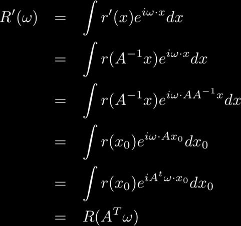
66 Radiance Transforms Optical elements transform rays They also transform radiance Points in ray space Radiance before optical transform Radiance after optical transform

67 Radiance Transforms Any ray x after transform is related to original ray by Because of radiance conservation Since The radiance after optical transformation is related to the original radiance by:

68 Radiance Transforms The radiance after optical transformation is related to the original radiance by: What is that for translation? So

69 In Class Exercise The radiance after optical transformation is related to the original radiance by: What is that for a lens? So

70 Image Rendering Now that we have the lightfield (all of the light in a scene) how do we turn q and p into a picture? (A rendered image)? Use physics of lightfield and image formation

71 Image Rendering A traditional image is formed by integrating rays from all directions at each pixel A traditional image is rendered from a radiance according to

72 Capturing Radiance with Radiance Cameras

73 Capturing Radiance To capture radiance, we need to capture rays from different directions individually But sensors are not directional Rays from different directions need to be mapped to different positions (different pixels)

74 Pinhole Camera Rays can only enter camera at one point (q = 0) Rays from different directions spread apart inside camera And are captured at different positions on the sensor Switches direction and position Captures angular distribution of radiance

75 Pinhole camera More precisely Switches angle and position Captures angular distribution of radiance

76 2F Camera Generalizes pinhole camera Lens of focal length f is placed at distance f from sensor Switches angle and position Captures angular distribution of radiance assuming it doesn t change much with q (close to q = 0)

77 2F camera This is the lens generalization of the pinhole camera Three optical elements: space, lens, space Scene Transformation:

Show that D is the aperture diameter Switches angle and

78 2F camera This is the lens generalization of the pinhole camera Three optical elements: space, lens, space Scene Show that D is the aperture diameter Switches angle and position Captures angular distribution of radiance (at q = 0)

79 Traditional 2D camera Three optical elements: space, lens, space Show that approximately.

80 Capturing Radiance Pinhole camera or 2F camera capture an image I(q) I(q) captures angular distribution of radiance Only for small area around q = 0 so far For complete radiance, we need to capture angular distribution for all q Basic Idea: Replicate pinhole or 2F at every q Ives (pinhole) Lippmann ( 2F )

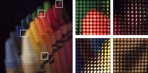
81 Ives Camera At the image plane: Multiplexing in space: Each pinhole image captures angular distribution of radiance. All images together describe The complete 4D radiance.

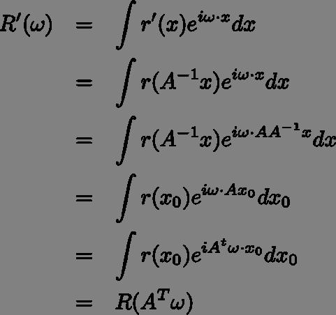
82 Radiance in Frequency Domain In the frequency domain, the two optical elements switch places: lens becomes space; space becomes lens

83 Radiance Transforms (Frequency Domain) Converting radiance into frequency representation gives us a new tool for analysis, and new power. A pixel no longer stands by itself, representing a point in one single image / slice in 4D radiance. In the frequency domain one pixel can represent multiple images at the same time. Those images are slices of the 4D radiance, but now in the frequency domain. By optically combining multiple frequencies, we achieve new and more efficient use of the sensor.

84 Radiance Transforms (Frequency Domain) Radiance in frequency representation: where and Next we derive the relation between and due to optical transform

85 Radiance Transforms (Frequency Domain)

86 Radiance Transforms Main results (summary): Note: Shear is in the other direction in frequency domain due to the transposed matrix. Lens <-> space. Note: The inverse always exists because det A = 1.

87 Ives Camera: Frequency Multiplexing Poisson summation formula train of delta functions = train of frequencies Prove

88 Ives Camera: Frequency Multiplexing Transposed translation f

89 Ives Camera: Frequency Multiplexing Band limited radiance Veeraraghavan s idea:

90 Cosine Mask Camera (MERL) A transparency, superposition of cos terms, is placed at distance f from the sensor Consider for example: Derive the expression for the radiance at the sensor:

91 Periodic Mask Camera (Adobe) Input:

92 Periodic Mask Camera (Adobe) Output:

93 Ives camera: Multiplexing in frequency

94 Ives camera: Multiplexing in frequency

95 Ives camera: Multiplexing in frequency

96 Lippmann s Camera Space multiplexing Lenses instead of pinholes A 2F camera replaces each pinhole camera in Ives design

97 Lippmann s Camera Heterodyning Frequency multiplexing or heterodyning analysis can be done in two steps: 1. Consider array of shifted pinhole-prisms with constant shift a, and prism angle a/f 2. Superposition of arrays with different shifts to implement microlenses as Fresnel lenses.

98 Lippmann s Camera Heterodyning Starting with Derive the radiance at the focal plane Show that at zero angular frequency it becomes:

99 Lippmann s Camera Heterodyning (derivations)

100 Lippmann s Camera Heterodyning (derivations)

101 Lippmann s Camera Heterodyning Video: Integral camera with frequency multiplexing Thanks to Ren Ng for providing the lightfield image.

102 Lippmann s Camera Heterodyning

103 Radiance Cameras with External Optical Elements

104 Arrays of Lenses and Prisms The most popular light-field camera is simply an array of conventional cameras. Alternatively, an array of lenses with a common sensor.

105 Arrays of Lenses and Prisms Shifting cameras from the optical axis means: We need to extend the vector space treatment to affine space treatment. Prism transform Shifted lens Lens + prism Those are equal

106 Adobe Camera Arrays of Lenses and Prisms Camera designs based on the above idea:

107 Adobe Camera Arrays of Lenses and Prisms

108 Mosquito Net Camera

109 Mosquito Net Camera Demo

110 Hands On with Radiance Cameras

111 Handheld Plenoptic Camera

112 Computational Methods for Radiance

113 Radiance Representation I(q) is an image Represents sampled lightfield Position is sampled by microlenses as pixels

114 Radiance Representation I(q) is an image Represents sampled lightfield Position is sampled by microlenses Direction is sampled by sensor pixels

115 Radiance Representation I(q) is an image Represents radiance sampled in position and direction

116 Radiance Representation

117 Radiance Representation 4D array 2D array of 2D arrays Position major q p

118 Radiance Representation

119 Radiance Representation 4D array q 2D array of 2D arrays Direction major p

120 Creating Radiance Array Given 2D flat captured by radiance camera Create 4D array Sample the same directional pixel from every position

121 Creating Radiance Array Given 2D flat captured by radiance camera Create 4D array If 2D position major flat happens to be regular (jnds,inds) = mgrid[0:height:nump,0:width:nump] for j in range(0,nump): for i in range(0,nump): radiance[:,:,j,i] = image[jnds+j,inds+i] Python, matlab very similar Samples the same directional pixel from every position

122 Creating Radiance Array Given 2D flat captured by radiance camera Create 4D array Sample the same positional pixel from every direction

123 Creating Radiance Array Given 2D flat captured by radiance camera Create 4D array If 2D direction major flat happens to be regular (jnds,inds) = mgrid[0:height:numq,0:width:numq] for j in range(0,numq): for i in range(0,numq): radiance[j,i,:,:] = image[jnds+j,inds+i] Python, matlab very similar Samples the same positional pixel from every direction

124 Aside: Dimensionality How large of a sensor do we need to capture radiance? Memory, computation requirements? What is a reasonable size for a rendered image?

125 Image Rendering A traditional image is formed by integrating rays from every direction at each pixel

126 Image Rendering Integration is averaging over directions at each position

127 Image Rendering Integration is averaging over directions at each position for j in range(0, nump): for i in range(0, nump): rendered[:,:] += radiance[:,:,j,i] rendered /= (nump * nump)

128 Rendering New Images Averaging recovers traditional image Can also render new images Different aperture Different viewpoint Different focus

129 Different Aperture A smaller aperture is a smaller set of directions

130 Different Aperture A smaller aperture is a smaller set of directions for j in range(alpha, nump-alpha): for i in range(alpha, nump-alpha): rendered[:,:] += radiance[:,:,j,i] rendered /= ((nump-alpha) * (nump-alpha))

131 Pinhole Rendering (single viewpoint) Only render from one pixel rendered[:,:] = radiance[:,:,j,i]

132 Different Viewpoints Different viewpoint is different direction Render different directions (or sets of directions)

133 Different Viewpoints Different viewpoint is different direction Render different directions (or sets of directions)

134 Different Viewpoints Different viewpoint is different direction Render different directions (or sets of directions)

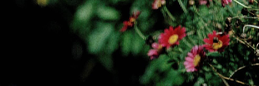
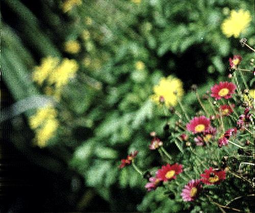
135 Orchard

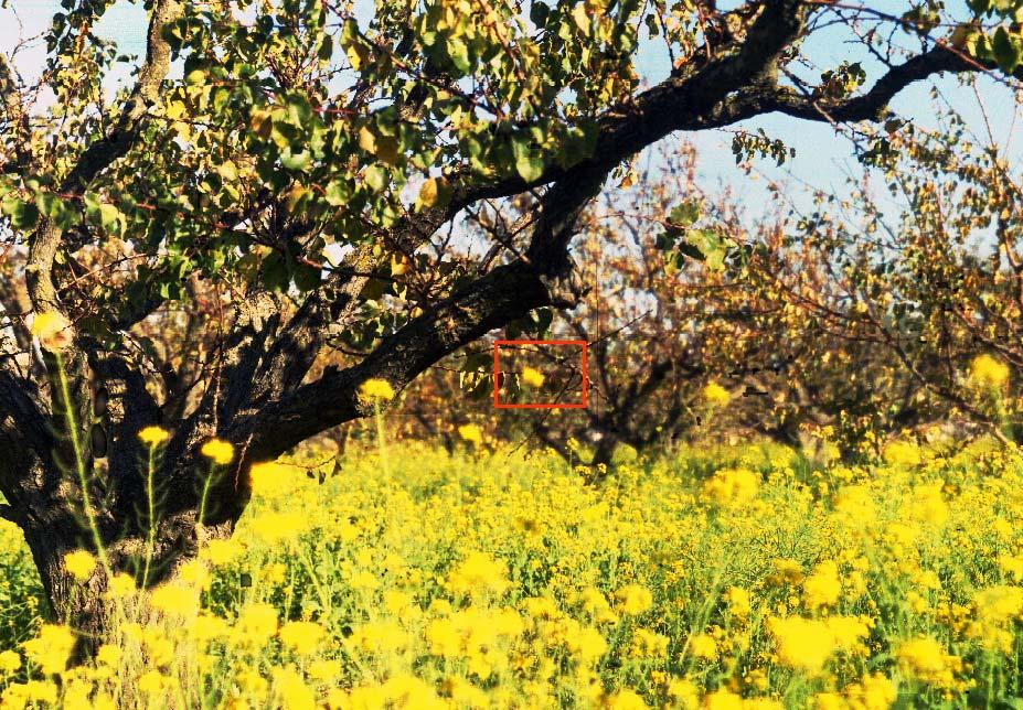
136 Orchard

137 Orchard

138 Orchard

139 Refocusing When we refocus a camera, we change the distance from the lens to the sensor Same object is no longer in focus.

140 Computational Refocusing Change the distance (translate) computationally Two different radiances, r1 and r2

141 Computational Refocusing We capture radiance r1. How can we compute r2? We need translation transform of the radiance.

142 Algorithm: Computational Refocusing Apply shearing transformation: Then render the new image:

143 Algorithm: Refocusing (yind,xind,wind,vind) = mgrid[0:m,0:n,0:r,0:s] shear_y = y + t*wind / r shear_x = x + t*vind / s rad_p = interpolate(rad, [shear_y, shear_x, wind, vind])

144 Fourier Slice Refocusing Ng 2005

145 Efficient Computational Refocusing Refocusing in the spatial domain requires operations for each refocused image An alternative approach (invented by Ren Ng) requires for initial setup but then for each rendered image we need only Insight: Refocus in the frequency domain The frequency domain representation of the rendering integral is the DC directional component (slice)

146 Transform of Rendered Image The Fourier transform of a rendered image: Recall that Thus we have In other words, the transform of the rendered image is the DC directional component of

147 Translation in the Frequency Domain Recall In the case of translation But we are interested in the case I.e., The refocused image is just a slice (with slope t)

148 Algorithm: Fourier Slice Refocusing Take FFT of radiance: Interpolate to get a slice: Take inverse FFT

149 Algorithm: Fourier Slice Refocusing radiancefft = fftn(radiance) (yind,xind) = mgrid[0:m,0:n] vind = t*yind / m uind = t*xind / n slice = interploate(radiancefft, [yind, xind, vind, uind]) rendered = ifft2(slice)

150 Demo: Fourier Slice Refocusing

151 Demo: Fourier Slice Refocusing

152 Demo: Fourier Slice Refocusing

153 Demo: Fourier Slice Refocusing

154 Demo: Fourier Slice Refocusing

155 Demo: Fourier Slice Refocusing

156 Plenoptic Camera 2.0 (See Supplemental Slides)

157 Wrap Up Questions answered Issues explored

158 References

159 Recommended reading Reading material has been selected for its educational value Many important references have been dropped in the effort to make this reading list short

160 Reading material GERRARD A., BURCH J. M.: Introduction to matrix methods in optics. GUILLEMIN V., STERNBERG S.: Symplectic techniques in physics IVES F., US Patent 725,567. (Year: 1903) LIPPMANN, G., Epreuvesreversibles, J. Phys. 7, pp , (1908)

161 Reading material

Computational Methods for Radiance. Render the full variety offered by the direct observation of objects. (Computationally).

Computational Methods for Radiance Render the full variety offered by the direct observation of objects. (Computationally). Methods for Plenoptic 1.0 Computing with Radiance Goal: Render the full variety