iric Software Changing River Science River2D Tutorials

Transcription

1 iric Software Changing River Science River2D Tutorials

2

3 iric Software Changing River Science Confluence of the Colorado River, Blue River and Indian Creek, Colorado, USA 1

4 TUTORIAL 1: RIVER2D STEADY SOLUTION OF THE CONFLUENCE OF THE COLORADO AND BLUE RIVERS This tutorial employs data collected at the confluence of the Colorado and Blue Rivers near Kremmling, CO. An aerial overview of the area of interest is shown below. This tutorial explores the basic functionality of iric for unstructured grids using the River2D solver. In this tutorial you will import data including topography, measured water-surface elevations, and a Background image. You will build a unstructured grid and apply boundary conditions to the grid. You will initialize and run the model and visualize the results. Flow direction Area of interest Colorado River Blue River 2

5 Contents TUTORIAL 1: RIVER2D STEADY SOLUTION OF THE CONFLUENCE OF THE COLORADO AND BLUE RIVERS Getting Started Preparing Bathymetric Data Creating the Computational Mesh Defining Inflow and Outflow Boundaries Bed Resistance Model Running the Model Visualization of Results Refining the Solution

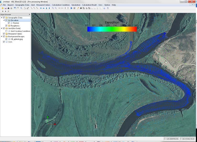
6 1. Getting Started iric s basic concepts and terminology can be found in the FaSTMECH solver Tutorial 1 and it is assumed you have already completed that tutorial for a basic understanding of how to import data, build grids, run the solver and visualize the results. 2. Preparing Bathymetric Data Start iric with a new project and select River2D in the Select Solver window. In the first step we are interested in importing the bathymetric and topographic information into iric, which is located in file CB_topo.tpo. Use command Import Geographic Data Elevation from the main menu bar and select file CB_topo.tpo to load the topographic information. Remember that the file has extension.tpo, which must be set appropriately in the filter of the Select file to import window. Leave the Filtering Setting to 1 (Fig. 2.1) and click Ok. A TIN will be created for the loaded data. After some zooming to the area of interest with the main toolbar tools and (recall that zooming in and out can also be accomplished by rotating the mouse wheel), the results look as shown in Fig Figure 2.1 In this tutorial, the visual feedback to build the SToRM simulation will be given by a georeferenced image, which is located in file CB_aphoto.jpg. Load the image into iric using the command Import Background Image from the main menu bar and selecting file CB_aphoto.jpg. The area of interest for this tutorial is the immediate neighborhood of the confluence of the two rivers. Pan and zoom to the area of interest to maximize the useful area of the canvas. iric should look like Fig It is now a good time to save your work 4

7 Figure 2.2 Figure 2.3 5

8 3. Creating the Computational Mesh The first stage in the preparation of a River2D run consists in defining the computational domain and grid. River2D uses an unstructured type of computational grid based on triangles, therefore set the grid to unstructured mesh: Use command Grid Select Algorithm to Create Grid to select Create grid from polygonal shape. Click OK. The computational domain is defined by a polygon that encompasses the area of interest. Define it by left-clicking the mouse at the desired polygon vertices. Double-click the last point or press <Enter> to finish the polygon. In this example we are interested in the region in close proximity to the confluence of the two rivers. Use Fig. 3.1 to guide you to create the mesh polygon. It is possible to edit (delete and add) and change the location of the vertices of the grid polygon. To accomplish these operations do the following: Left click on Grid Creating Condition in the Object Browser window. This will activate the editing menu bar. Next, in the graphics view use the mouse to left click on the polygon you just created. This activates the polygon and its vertices appear as black squares. The mouse can now grab individual vertices: when left clicking the vertex, the cursor changes from an open hand shape to a closed hand shape, which means it is grabbing that vertex. After any action you can undo you move by selecting the undo button in the Main Toolbar. Select a vertex and move the mouse without releasing the left button and the vertex will move with it. Release the mouse button at the desired new vertex location. This process is depicted in Fig. 3.2, where the cursor is placed near a vertex and takes the shape of an open hand (Fig. 3.2, left), then the mouse is clicked and the vertex is moved (Fig. 3.2, right). Grabbing near or on top of a vertex moves the vertex; grabbing the frame moves the entire polygon to a new location. New vertices can be added to the grid polygon: left click on the button, then left click on the desired location for the new vertex. This location must be on the polygon, and not inside or outside of it. Similarly, and existing vertex can be deleted from the polygon: left click on the then left click on the vertex to be deleted. button, The above operations can be undone using the undo button in the main toolbar. 6

9 Figure 3.1 Figure 3.2 In iric, the computational grid is generated automatically by a triangulation program that uses quality constraints specified by the user. To start the automatic mesh generator: Right-click on Grid [No Data] in the Pre-processing Window and select Create grid in the pop-up menu. The geometric constraints required by the mesh generator are specified in the pop-up window that appears. They relate to mesh quality: minimum internal angle and maximum area of the triangles, and are shown in Fig The first constraint avoids stretched triangles with poor interpolating properties. The second constraint defines their maximum size, in area (m 2 ) (the mesh generator sets the triangles size based on boundary conditions, on mesh smoothness, and on the quality requirements just defined). It is desirable to create a mesh with the appropriate density: too many triangles and the run takes too long, too few and the flow is under-resolved. The triangles area is the parameter used by the mesh generator to control the density of the grid. Both constraints are used in this tutorial, as indicated by the checkmarks in the respective check boxes, as shown in Fig The triangle area can be set by trial-and-error, until visual inspection indicates a good distribution of points in the computational grid. 7

10 Figure 3.3 The mesh generator runs and a pop-up window that allows the user to map the geographic data to the grid. Click Yes to continue. The result is shown in Fig Note the new name for the grid in the Object Browser window: Grid (3144). This indicates the number of elements used in this mesh. Figure 3.4 We can visualize the bed elevation mapped to the grid by checking Grid (3144) Node attributes Elevation in the Object Browser window. This is shown in Fig. 3.5, which was obtained after changing the default color pattern used. Changes to the color map are accomplished in the Grid Node Attribute Display Setting window, which can be reached by right clicking the mouse on Grid (3144) Node attributes Elevation and selecting Property in the pop-up menu. The particular numerical values corresponding to the colorization scheme chosen are presented in Fig

11 Figure 3.5 Figure 3.6 Finally, note that the grid must be generated anew every time that the grid polygon is changed. This is a good point to save your work (File Save or File Save As ). Remember to save often. 9

12 4. Defining Inflow and Outflow Boundaries The next step involves the definition of the inflow and outflow boundaries. In subcritical flow, the flow velocity is always specified at the inflow boundaries (i.e., the upstream-most cross sections) and the stage at the outflow boundaries (the downstream-most cross sections). There can be any number of inflow and/or outflow boundaries. Each boundary is defined by specifying a string of adjacent nodes located on the grid s bounding polygon. In this example, there are Three inflow boundaries at the right, and one outflow boundary at the left of the computational domain of Fig Flow is from right to left (i.e., from East to West). This section describes all the steps involved in defining the inflow boundaries and their associated parameters. It may be convenient to zoom in to the appropriate area of the domain to have a more detailed view of the mesh. The first inflow boundary is the inflow of the Colorado River. Zoom in the area of interest in the mesh boundary. Right-click on Boundary Condition item in the Pre-processing Window and select Add Inflow Condition in the pop-up window. Assign the inflow condition a name and click Ok. Here, we use Colorado (Fig. 4.1). In this case we will be using a Fixed Discharge of 10 m 3 /s. There are two methods for selecting the boundary condition nodes: 1. Left-click on the first node and then holding the Shift key to select the remaining nodes belonging to the outflow boundary. Do not skip nodes and select the nodes in order. When finished, right click the mouse in the Graphics View and select Assign condition from the pop-up menu. The defined inflow boundary is shown in Fig Use Ctrl + Left-Mouse Button to rotate the view such that the boundary is perpendicular to the horizontal or vertical direction and then select the boundary nodes by using the mouse to left click and drag a rectangle surrounding the boundary nodes only. When finished, right click the mouse in the Graphics View and select Assign condition from the pop-up menu. The defined inflow boundary is shown in Fig You can reorient the view by selecting in the Main toolbar. 10

13 Figure 4.1 Figure 4.2 Note that a new entry can be found in the Object Browser, under the Boundary Condition item. Each boundary will have a similar entry, with the name designated by the user. Repeat the same steps to define the second and third inflow boundaries for the Blue River and Indian Creek. Use the values shown in Fig. 4.3, i.e., use Q = 20 m 3 /s for the Blue River and Q = 1 m 3 /s for Indian Creek. The result is shown in Fig

14 Figure 4.3 Figure 4.4 For each inflow boundary condition a synthetic flow velocity field is then generated with velocity vectors that are perpendicular to the string. Due to the artificial nature of this velocity distribution, it is recommended that inflow boundaries should be placed away from areas of interest, where accurate solutions are sought. When possible, these boundaries should be constructed by placing the string of nodes perpendicularly to the channel centerline and away from curved flow areas and recirculation zones whenever possible. 12

15 It is also necessary to define the outflow boundaries. Each outflow boundary is the set of nodes that defines a downstream-most cross section of the modeled reach, where the flow exits the area being modeled. Outflow boundaries are defined following the same steps carried out when defining the inflow boundaries. Pan and/or zoom to the area where the boundary is located. Right-click on Boundary Condition item in the Pre-processing Window and select Add Outflow Condition in the pop-up window. Assign the outflow condition a name, here we use Outflow (Fig. 4.5). Enter the Fixed Elevation for the water surface elevation and click Ok. In this example, only one value is entered (Stage = m in Fig. 4.5). Left-click on the nodes belonging to the outflow boundary without skipping any. When finished, right click the mouse and select Assign boundary condition from the pop-up menu. The defined inflow boundary is shown in Fig Figure

16 Figure 4.6 Sometimes, it is easy to make an error creating a boundary-node string. Any string can be deleted by right-clicking on its name and selecting Delete in the corresponding pop-up menu. Similarly to what was recommended for the inflow boundary, the outflow boundary nodes should form a line perpendicular to the channel centerline, away from recirculation areas, and far downstream from the areas of interest in the study. Save your work. 5. Bed Resistance Model River2D uses a non-dimensional Chezy coefficient to close the stress terms. The Chezy coefficient (C s )is related to the effective roughness height k s as follows: C s = 5.75log[12 * (H/k s )] Where flow resistance is due primarily to bed material roughness, a good starting point for k s is 1-3 times the largest grain diameter. However, final values of roughness should be calibrated to measured water surface elevations. In iric roughness can be set by drawing polygons (sometimes called coverage polygons) over the areas of interest. Follow these steps to set the roughness: In the Pre-processing Window, under Geographic Data right-click on Roughness and select Add and Polygon in the respective pop-up menus. Draw a polygon covering the entire computational grid. Finish by double-clicking the last node of the polygon (or by pressing <Enter>). The polygon may look like what is shown in Fig Enter the value of the roughness, as in Fig

17 Map the roughness values to the computational grid by selecting from the Menu Bar Grid Attributes Mapping Execute. Figure 5.1 Figure 5.2 Only one coverage polygon is used in this example, but multiple polygons can be defined, each covering only some part of the computational grid. A roughness value must be given for each polygon, and all the grid nodes within that polygon will have the k s -value thus assigned. 6. Running the Model The River2D solver uses a set of parameters that must be specified by the user. These parameters concern the selection of the desired numerical techniques used in computing the flow solutions. This selection is accomplished in a series of entry screens described in this section. Model parameters are defined in the Calculation Condition window. In iric s menu bar, select Calculation Condition Setting to open the Calculation Condition window. Different groups of parameters can be defined by selecting the appropriate name on the left column. Enter the 15

18 parameters as shown in Figure 6.1. More information on each variable can be found in the River2D.pdf document. A B C D Figure 6.1 After the data preparation, River2D is run by clicking the run button ( ) on the main toolbar. A window pops-up (see Fig. 6.2) where the progress of the computation can be followed. At each iteration the following information is given: Current Time: the current time in seconds since the start of the calculation Time Difference: The time step used in the current iteration. Solution Change: The relative change in solution variables over the last time step. Total Inflow: Sum of all the inflow boundary conditions Total Outflow: Flow at the outflow boundary condition. This example takes approximately 10 minutes to run in an average desktop computer. Figure

19 A model run can be stopped while in progress. This is done by clicking on button in the main toolbar and clicking on Yes when prompted by the Confirm Solver Termination window. 7. Visualization of Results After the computations are completed, a visualization window can be open by issuing the command Calculation Result Open new 2D post-processing window or by clicking on the button in the main toolbar. Different quantities can be plotted by activating them in the left window pane called Object Browser. Figs. 7.1 through 7.3 show the results of this simulation: the water depth and computational grid in Fig 7.1; the velocity vectors and magnitude in Fig. 7.2; then the water surface elevation, and finally water depth. Only wetted computational cells are displayed. Save the project. Figure

20 Figure 7.2 Figure Refining the Solution 18

21 iric contains tools that allow the computational mesh to be easily refined and/or coarsened. A mesh is refined when the new mesh uses smaller triangles than the original, and coarsened when larger triangles are used. Refinement and coarsening of the computational grid is done selectively, i.e., the mesh is refined and/or coarsened only in selected areas of the domain. Selective refinement may be advantageous when only a small part of the reach needs a fine mesh, while the solution for the remainder of the reach can be obtained by the use of a larger mesh. Areas where finer grids are needed are areas where the variables (water and/or flow velocity) change rapidly, such as in recirculation areas behind obstacles, around the tip of groins or other salient features, etc. Using selective refinement is a good way to avoid having too many grid triangles where a few are enough, this reducing the total number of computational points, resulting in increased computational efficiency (i.e., River2D runs faster). Areas of mesh refinement and coarsening are created by defining polygons within the main mesh area. For this tutorial, we are interested in refining the solution in a small area at the confluence of the Blue and Colorado rivers. The refinement polygon is created in the same manner as when creating the main computational grid polygon. Before beginning save the project with a new name from the Menu Bar using File Save As. Left-click on Grid Creating Condition on the Object Browser of the Pre-processing Window. This will bring up a toolbar:. Use button to create a refinement polygon as shown in Fig Click <Return> (or double-click the last point) when completed. Figure 8.1 When asked by the Refinement maximum area window, use a maximum triangle area of 5 m 2 for this newly defined region and enter it in the pop-up window. Rebuild the mesh as before: rightclick on Grid (in the Object Browser panel) and select Create Grid from the pop-up menu. For the main grid, use the same parameters as those chosen earlier (Fig. 3.3). The resulting mesh is shown in Fig After the mesh is created: 19

22 Map attributes to the new grid: Grid Attributes Mapping Execute from the main menu. The inflow and outflow boundaries need to be redefined. Re-do the steps described in section 4 titled Defining Inflow and Outflow Boundaries. Fig. 8.2 shows the completed mesh, colorized by bed elevation and with the new boundary node strings. This new mesh has 4316 nodes. Figure 8.2 Open a post-processing visualization window to view the results using the button in the main toolbar (or the pull-down menu Calculation Result Open new 2D post-processing window in the main menu bar). Create a pair of figures to compare the solution between the Refined Grid and Unrefined Grid as follows: Create a figure of the velocity magnitude as shown in Figure 8.3A by using the Save Snapshot from the File menu or from the Main Menu toolbar. Open the previous project with the unrefined grid and create a similar figure as shown in Figure 8.3B. Insert the figures into a document and note the differences. 20

23 A B Figure