Stereo Vision Based Mapping and Immediate Virtual Walkthroughs

Transcription

1 Stereo Vision Based Mapping and Immediate Virtual Walkthroughs Heiko Hirschmüller M.Sc., Dipl.-Inform. (FH) Submitted in partial fulfilment of the requirements for the degree of DOCTOR OF PHILOSOPHY June 2003 School of Computing De Montfort University Leicester, LE1 9BH, UK.

2 For my wife Ranjna.

3 Abstract This thesis investigates stereo vision based techniques for supporting work with teleoperated mobile robots. In particular, the tasks of navigation and control of the robot in unknown environments as well as control of the manipulator are considered. Support is required with map overviews and images from novel viewpoints. Challenges are to create maps and novel images in real time, exclusively from image sequences of a calibrated stereo camera that is allowed to move arbitrarily in three dimensions. Furthermore, no assumptions are made about the environment. These requirements have led to research in the areas of stereo vision, camera motion estimation, mapping and novel view synthesis. Several contributions have been made in these areas. Firstly, the behaviour of stereo correlation is analysed and a new real time stereo algorithm derived, which has reduced matching errors compared to traditional algorithms. Secondly, a new robust real time camera motion estimation method is described, which exclusively uses stereo images and permits arbitrary camera motion. Thirdly, a new method for creating two-dimensional maps from images of a stereo camera under arbitrary three-dimensional motion is presented. Finally, novel view synthesis is performed in disparity space of source stereo images using a new method. All the proposed techniques have been integrated into the Immediate Reality Scanner (IRIS) system. The system performs incremental mapping, immediate virtual walkthroughs and dynamic novel views exclusively from a stereo camera under arbitrary three-dimensional motion. Mapping and immediate virtual walkthroughs can be performed in real time, concurrently to scanning the environment. The thesis describes camera calibration, stereo processing, camera motion estimation, map building, novel view synthesis and the integration into IRIS, including evaluations in all areas. It is concluded that IRIS does not only fulfil the requirements of the anticipated application on teleoperated mobile robots, but could also be used in a wide range of robotics and non-robotics applications. It is believed that IRIS is the first system that allows incremental mapping and immediate virtual walkthroughs in real time concurrently to scanning an unconstrained environment with an arbitrarily moving stereo camera. i

4 Contents Declaration Acknowledgements Notation x xi xii 1 Introduction Teleoperated Mobile Robots Aims and Constraints Contributions Organisation of Thesis The Stereo Camera Model Introduction Related Literature Modelling Cameras Model Definition The Calibration Grid Single Camera Calibration Stereo Camera Calibration Transformation into an Ideal Model Model Definition Planar Rectification Evaluation of Calibration and Rectification The Stereo Hardware Accuracy of Calibration Point Localisation Accuracy of Calibration and Rectification Speed of Rectification Conclusion ii

5 CONTENTS iii 3 The Stereo Algorithm Introduction Related Literature Analysis of Stereo Correlation General Behaviour Behaviour at Depth Discontinuities and with Small Objects Confirmation of Assumed Behaviours Fast Correlation with Reduced Matching Errors Overview Multiple Supporting Correlation Windows Correlation Function Error Filter Border Correction Filter Segment Based Interpolation Evaluation of the Stereo Algorithm Comparison of Correlation Measures Effect of Correlation Function Error Filter Effect of Border Correction Filter Effect of Segment Filter and Interpolation Results of Combinations of Proposed Methods Speed of the Stereo Algorithm Conclusion Reconstruction and Modelling of Errors Introduction Related Literature Reconstruction from Disparities Distribution and Calculation of Reconstruction Errors The Image Based Error Model The Spherical Error Model The Ellipsoid Error Model The Ellipsoid Error Model with Drift Compensation Propagation of Errors The Error in the Coordinates of a Reconstructed Point The Error in the Distance from the Camera The Error in the Distance Between Two Reconstructed Points Conclusion

6 CONTENTS iv 5 Camera Motion Estimation Introduction Related Literature The Stereo Constraint Satisfaction Method Overview Finding Initial Correspondences Outlier Detection Calculation of Transformation Evaluation of Camera Motion Estimation Determination of Consistent Correspondences Accuracy of Motion Calculation Dependency of Accuracy on Frame Rate Speed of Camera Motion Estimation Conclusion Map Building Introduction Related Literature A Fuzzy Logic based Layered Occupancy Grid Overview Geometry of the Occupancy Grid Updating of the Occupancy Grid Creation of Visual Maps Evaluation of Map Building Mapping of a Simple Scene Mapping of Real Scenes Speed of Map Building Conclusion Novel View Synthesis Introduction Related Literature Novel View Synthesis in Disparity Space Overview Selection of Source Views Creation of Rays in Disparity Space Intersection of Rays with the Disparity Surface Fusion of Pixel Values

7 CONTENTS v 7.4 Evaluation of Novel View Synthesis Prediction of Views Speed of Novel View Synthesis Conclusion Overall System and Experimentation Introduction Related Literature The IRIS Prototype System Overview Mapping and Virtual Walkthroughs for Large, Static Environments Dynamic Novel Views for Local, Changing Environments Evaluation of IRIS Scope of Evaluation Evaluation of Mapping and Virtual Walkthroughs Evaluation of Dynamic Novel Views Conclusion Discussion and Conclusion Discussion Fuzzy Logic versus Probability Theory Backward versus Forward Mapping Increasing Accuracy Conclusion Recommendations 132 References 134 A Appendix 148 A.1 Abbreviations A.2 Hardware Specification A.3 Selecting the m Lowest out of n A.4 A Brief Introduction into Fuzzy Logic A.5 Memory Efficient Implementations of Occupancy Grids A.6 Implementation of IRIS A.6.1 General Remarks A.6.2 Structure of Programs A.6.3 Structure of the Stereo Vision Library

8 List of Tables 3.1 Results of SAD correlation on Tsukuba images Errors at borders, using SAD on Tsukuba images Partial derivatives of reconstruction equations Description of 5 closed stereo image sequences Frame rates of mapping and virtual walkthroughs Frame rates of dynamic novel views A.1 Specifications of cameras A.2 Specifications of frame grabbers vi

9 List of Figures 1.1 High level structure of a teleoperated mobile robot system Organisation of the thesis Image of calibration grid and determination of calibration points Projection of pixels from individual image planes onto a common plane The used stereo camera Error of calibration point localisation Errors after calibration and after rectification Errors in distance and disparity of measuring distances Speed of rectification of one stereo image pair of size Stereo correlation at the border of an object Typical decision conflict at an object border Tsukuba stereo image with ground truth Magnified part of Tsukuba images and calculated disparity image The MWMF stereo algorithm, with new parts shown in grey Proposed configurations of multiple correlation windows A typical correlation function for a dissimilarity measure Derivation of border correction filter Slanted stereo image with ground truth Comparison of correlation methods on Tsukuba images Comparison of correlation methods on Slanted images SAD correlation on Tsukuba images Rank correlation on Tsukuba images MW-SAD correlation on Tsukuba images SAD5 (i.e. SAD with 5 supporting windows) correlation on the Tsukuba images Filtered errors and correct matches at certain thresholds SAD correlation with Border Correction Filter on Tsukuba images SAD correlation with Segment Filter and Interpolation on the Tsukuba images vii

10 LIST OF FIGURES viii 3.19 Stepwise combination of all proposed methods Result of using all new methods together on the Tsukuba images Speed of individual components of the MWMF stereo algorithm Distribution of the image based error ε di Reconstruction of a point from two different stereo camera viewpoints Comparison between the image based and ellipsoid error Calculation of the centre of an ellipsoid error contour for a specific error Comparison between image based and propagated errors Ratio of the propagated distance error and its approximation The complete SCS camera motion estimation method Finding initial corresponding feature points by correlation Matrix m, which stores the consistencies of all pairs of corresponding points The complete seminar room sequence with arbitrary motion The number of corners and correspondences in the seminar room sequence Some images of 5 closed stereo image sequences Motion error of all sequences with different error models Camera path with different error models on the seminar room sequence Problematic, consecutive images of the bedroom sequence Motion error in dependency of the frame rate Speed of individual components of the SCS method Overview over the FLOG mapping method The layered occupancy grid Membership functions for emptiness E i and occupancy O i for point P i Mapping of two simple objects Four stages of an incrementally created map Mapping of closed sequences, with different error models Mapping of two long sequences Speed of FLOG mapping method Basic concept of novel view synthesis in disparity space Overview over the DSNV method Three-dimensional boundaries of source and novel view Definition of the search range on the ray Intersection between a ray and the disparity surface Three cases, if the ray is projected as a point in the source view Prediction of images from stereo views of the box sequence

11 LIST OF FIGURES ix 7.8 The combination of source images with different brightness can lead to spots Novel views of a head with different resolutions and at different angles Speed of DSNV method using stereo view of head ( pixel) Embedding of IRIS into a teleoperated mobile robot system IRIS system architecture for static environments IRIS system architecture for dynamic situations Concurrent mapping and virtual walkthroughs on different sequences Processing time distribution of concurrent mapping and virtual walkthroughs Three stages of dynamic novel views on grasping sequence Processing time distribution of dynamic novel views on grasp sequence A.1 Memory efficient data structure for occupancy grids A.2 User interface of calibration and viewer program A.3 Structure of calibration and viewer program A.4 Structure of command line tools A.5 Relationships between all modules of the stereo vision library

12 Declaration I hereby declare that this thesis is a record of work undertaken by myself and is not being submitted concurrently in candidature for any other degree. Heiko Hirschmüller x

13 Acknowledgements I would like to thank my supervisor Peter Innocent for permanently offering encouragement and advice. His efforts are greatly appreciated. I would also like to thank Jon Garibaldi and Robert John for their participation in the supervision team. Furthermore, I am very appreciative for the relaxed working atmosphere at the Centre for Computational Intelligence, which enabled me to completely focus on this research. I would like to thank Chris Czarnecki for inspiring this project. Moreover, I thank Bill Nelson and Steven Lee at QinetiQ Farnborough not only for funding this project, but also for providing an interesting real world application and for inspiring discussions. On a personal note, I would like to thank my parents for raising me with love and supporting my own choices in life. My thanks also go to all other family members and friends who supported me during this time. Finally, I convey my deepest gratitude to my wife Ranjna Sharma-Hirschmüller for her patience and constant support. She always put my work first and motivated me in difficult times. I would have found it impossible to devote that much energy and time in this research without her constant love and understanding. xi

14 Notation Points, Vectors and Matrices p, q Points in 2D coordinate system P, Q Points in 3D coordinate system P Distorted point in camera coordinate system P Undistorted point in camera coordinate system p Image point in homogenous coordinates p Rectified image point R Rotation matrix (size 3 3), with elements r ik T Translation vector (size 3) J K Jacobian matrix Covariance matrix m, b Parameters of a line Camera Model Parameters A Camera projection matrix (size 3 3) t f γ o x, o y k 1, k 2 M Focal length in pixels Baseline in mm Skew Correlation Coordinates of the principal point Coefficients of radial lens distortion Symbolises the single camera model L, R Areas in the left and right images L Alternative area in the left image C Correlation value xii

15 NOTATION xiii c L R Correlation of two areas Errors and Probabilities ε σ S P Specific error Expected or propagated error Standard deviation Numerically estimated standard deviation Error function (i.e. normal error integral) Fuzzy Logic µ x Membership to fuzzy set x E, O, K Fuzzy set for emptiness, occupancy and confidence I, M Fuzzy set for indeterminateness and visual map C Cell of occupancy grid N Number of updates Common Indices x, y, z Indices for X, Y or Z coordinate d Index for disparity l, r, s Indices for left, right and stereo n Index for novel view i, j, k Miscellaneous indices Miscellaneous s General scale factor l O Distance φ, θ Angles The number of algorithmic steps n, m Number of elements

16 1 Introduction 1.1 Teleoperated Mobile Robots Teleoperation is the activity of carrying out tasks from a distance. Teleoperator systems are used to perform tasks in remote environments that are too distant, dangerous or inaccessible for humans [133]. A special subclass are teleoperated mobile robots, which allow free movements in a remote environment. Figure 1.1 shows the high level structure of a teleoperated mobile robot system. The main control loop of the system consists of the operator, the local computer based control system and the remote mobile robot, which typically has also some computational power on-board. The operator issues commands for controlling the robot or manipulator, which are transmitted from the local computer to the mobile robot. Sensor information from the mobile robot (e.g. video signal) are transmitted back to the operator to observe the progress of the work. Generally, there are two more control loops. The local control loop consists of the operator and the local computer and is used for planning and simulating work. The remote control loop consists of the mobile robot and its on-board computer and is used for performing certain minor tasks autonomously. Operator Local computer Mobile robot Camera Manipulator Commands, actions Remote Environment Sensor feedback (e.g. video signal) Figure 1.1: High level structure of a teleoperated mobile robot system. Applications of teleoperated mobile robots include explosive ordnance disposal, mine clearance, hazardous waste handling, decontamination, etc. The individual application environment might be known to the operator and there might be the possibility to observe the mobile robot directly or through cameras. However, this thesis considers application environments that are unknown to the operator and can not be seen directly (e.g. inside a house). Furthermore, it is assumed that the environment is not engineered for teleoperated work (e.g. no cameras in the environment that could observe the robot). Thus, the movements of the robot and the manipulator can only be observed through the on-board camera of the mobile robot. This camera has an unfavourable 1

17 CHAPTER 1. INTRODUCTION 2 viewpoint for navigation of the robot as it does not provide an overview. Furthermore, the viewpoint is relatively close to the manipulator, which makes judging distances and three-dimensional relationships difficult and results in poor manipulator control. There are a variety of possibilities for improving the performance of a teleoperated system (i.e. making it easier and faster to use). One possibility is to increase usability with generic operator interfaces or semi-autonomous control modes [54]. Other improvements concentrate on better visual representations of the environment and its relationship to the robot or manipulator [35, 101, 127], thus improving the feedback from the robot. The focus of this thesis is on supporting navigation and control of the mobile robot as well as the manipulator using novel visual representations. The navigation task involves high level planning to move the robot from its current location to a target location through an unknown environment. This can be supported with a map overview of the environment that also shows the current position and orientation of the robot. Controlling the robot can benefit from viewing it in the environment from arbitrary viewpoints (i.e. as if the operator would stand next to the robot for observing its movements from any desired position). Virtual representations are very useful for understanding local three-dimensional structures and relationships. This leads to the idea of creating a virtual representation immediately from sensor data and performing an immediate virtual walkthrough to observe the environment and robot. The environment is in these cases supposed to be static as the robot travels through it. However, this assumption becomes invalid as soon as the manipulator is used to perform tasks in the environment that change it. Nevertheless, a novel viewpoint that is not constrained to be on-board the mobile robot is in this case also beneficial and can help judging distances and three-dimensional relationships. This will be called a dynamic novel view, because the environment is dynamic. Challenges are the creation of all visual representations (i.e. maps and images from novel viewpoints) in real time from sensors that are travelling on-board the mobile robot. Sensors must deliver visual information (i.e. images) as well as the corresponding three-dimensional structures for virtual representations. This can be achieved by combining a camera with a three-dimensional laser scanner or by using a stereo camera. Measurements by laser scanners are generally more precise than stereo vision, but three-dimensional laser scanners can be very expensive, big and slow compared to stereo vision. Therefore, a stereo camera will be used as sensor. Hence, the considered problem is described as creating incremental maps, immediate virtual walkthroughs and dynamic novel views in real time from image sequences of a stereo camera. Section 1.2 defines the aims and constraints of the thesis precisely. A summary of the main contributions of this research is described in Section 1.3. Finally, the organisation of the thesis is discussed in Section 1.4.

18 CHAPTER 1. INTRODUCTION Aims and Constraints The aim of the research described in this thesis is to create map overviews and images from arbitrary viewpoints in real time exclusively from stereo image sequences. This involves research in the areas of stereo vision, camera motion estimation, mapping and novel view synthesis through image based rendering (IBR). The aim is achieved by devising novel methods or refining existing ones to reduce errors, increase accuracy and robustness while considering real time suitability. The application of these techniques is the creation of map overviews and immediate virtual walkthroughs to support navigation and control of a teleoperated mobile robot. Furthermore, manipulator control has to be supported with dynamic novel views. However, the scope is limited to the physical and technical problems of recovering and providing the described visual representations. All human computer interaction aspects and the concrete integration into a teleoperated control system are outside the scope of this work. There are a number of constraints that have to be considered for the anticipated target application. Only one calibrated stereo camera is used as sensor (i.e. no other sensors are assumed). This ensures the independence from robotic systems with specific capabilities and increases the portability and general usage. Arbitrary three-dimensional camera movements have to be anticipated as the robot might travel on rough ground or the camera might be mounted on the manipulator. All operations must be performed in real time, concurrently to the collection of a stereo image sequence. A frame rate of 5-10 fps for processing stereo images and creating visual representations is considered sufficient for a human operator (for the anticipated application). All techniques should work with cost-efficient hardware (i.e. cameras and computer). This prohibits the use of specialised cameras for increasing accuracy or fast processing boards for increasing speed. It is assumed that the environment is mostly static for tasks like navigation and robot control, because the robot is supposed to travel passively through the environment to target locations. However, dynamic environments must be anticipated at target locations, because the environment will be actively changed with the manipulator. It is also assumed that the environment contains at least some kind of visual features or textures. However, there can be no further assumptions about the environment made. In particular, it might be structured, unstructured or a mixture of both.

19 CHAPTER 1. INTRODUCTION Contributions The main contribution of this research is the presentation of the Immediate Reality Scanner (IRIS). IRIS is the first system that allows incremental mapping, immediate virtual walkthroughs and dynamic novel views concurrently to the real time processing of stereo image sequences from a camera under arbitrary three-dimensional motion in unconstrained environments. The development of IRIS involved investigations into the areas of stereo vision, camera motion estimation, mapping and novel view synthesis. Significant contributions have been made in each of the four areas. Firstly, an investigation into the problems of stereo correlation (i.e. errors at object borders and general matching errors) has led to an understanding of the behaviour of stereo correlation, especially at object borders. A new multiple window configuration and several filters that tackle problems individually have been derived form the analysis. This has resulted in the Multiple Window, Multiple Filter (MWMF) real time stereo algorithm [63, 66]. The method has been compared to other stereo algorithms in an independent study [126], which has recommended it as a very good choice if processing time is an issue. Secondly, an investigation into camera motion estimation for stereo cameras that move arbitrarily in three dimensions has led to a robust method for finding reliable correspondences between highly differing consecutive stereo images. The method is based on the satisfaction of certain constraints and works without any predictions or assumptions about camera motion. The research also included a review and comparison of different error models of the reconstruction error, which is important for the definition of constraints and accurate calculation of camera motion. This has led to the Stereo Constraint Satisfaction (SCS) method [65], which determines robustly and in real time the camera motion exclusively from a sequence of stereo images. Thirdly, the problem of creating a two-dimensional map overview from stereo sequences of a camera that moves arbitrarily in three dimensions has been studied. This has resulted in the Fuzzy Logic based Layered Occupancy Grid (FLOG) method [64], which is memory efficient and can be used in real time applications. Finally, the problem of creating novel views in real time at arbitrary viewpoints from a collection of stereo views has been examined. The problems of existing novel view synthesis techniques have been studied and a Disparity Space based Novel View (DSNV) method proposed. The method does not require any pre-processing time or additional memory and its speed can directly be scaled by reducing the image resolution. Furthermore, virtual objects can be drawn into novel images. 1.4 Organisation of Thesis The organisation of the thesis is depicted in Figure 1.2. The Chapters 2, 3 and 4 discuss all required techniques to recover the three-dimensional scene structure from one stereo image. Chapter 2 reviews the stereo camera model and discusses calibration and rectification. The accuracy for per-

20 CHAPTER 1. INTRODUCTION 5 forming measurements with the used hardware is also determined. Chapter 3 is concerned with the determination of correspondences between images and introduces a new real time stereo algorithm. Reconstruction is shown in Chapter 4 and different models for the reconstruction error reviewed. Individual stereo views are related by estimating the motion of the camera between consecutive stereo views. A new method for camera motion estimation is explained in Chapter 5. This results in a collection of stereo views, which describe the visual representation of a scene as well as its three-dimensional structure. Recovering 3D structure of environment with list of stereo views Recovering 3D structure from one stereo image Chapter 2 Chapter 3 Chapter 4 Chapter 5 Stereo Camera Model (Calibration, Rectification) Stereo Algorithm (MWMF) Reconstruction and Modelling of Errors Camera Motion Estimation (SCS) Collection of stereo views Chapter 6 Map Building (FLOG) Chapter 7 Novel View Synthesis (DSNV) Incremental maps Chapter 8 Overall System and Experimentation (IRIS) Immediate virtual walkthroughs and dynamic novel views Figure 1.2: Organisation of the thesis. Chapters 6 and 7 describe two techniques that use the collection of stereo views to create different kinds of visual representations of the environment. Chapter 6 proposes a new method for creating two-dimensional map overviews incrementally from stereo views. Chapter 7 uses the collection of stereo views for creating novel views at arbitrary viewpoints. Mapping and novel view synthesis are combined in Chapter 8, which describes the integration of incremental maps with virtual walkthroughs and dynamic novel views. Evaluations for the anticipated target applications are provided as well. The thesis is concluded in Chapter 9 and recommendations for future work are given in Chapter 10.

21 2 The Stereo Camera Model 2.1 Introduction The aim of this research is to use stereo vision for creating maps and novel images. This involves measuring the three-dimensional structure of the scene from stereo images. Performing accurate measurements with cameras requires a mathematical model that describes the projection of the scene onto the camera images. The parameters of the model are determined with a calibration process. Furthermore, it is important to determine the accuracy with which three-dimensional measurements can be performed. This Chapter discusses related literature in Section 2.2 and the model and calibration of stereo cameras in Section 2.3. The resulting camera model is complex and impractical to use. However, it is possible to transform it into an ideal model with desirable properties. Section 2.4 describes the ideal model as well as the transformation process, which is called rectification. The ideal model of rectified cameras is of great importance for stereo vision and used throughout the thesis. Section 2.5 evaluates calibration and rectification and determines the calibration error and the accuracy with which distances can be measured. 2.2 Related Literature Cameras are commonly described by a pinhole model in which all rays of light go through one point, i.e. the optical centre. Real cameras do not exactly correspond to this model due to the thickness of the lens. However, it is generally acknowledged that the pinhole model is a very good approximation [36]. Pinhole models consist of a linear part that performs the projection and a non-linear part that corrects lens distortion. Lens distortion is an unwanted side effect of camera lenses that bends straight lines. The treatment of lens distortion distinguishes between different pinhole models. Early models did not include lens distortion at all [1], while it is today commonly described using a radial distortion model [39], with one [68, 148] or two coefficients [134, 160]. More complex models additionally treat tangential distortion with two coefficients [62, 90] to improve accuracy. Beyer [8] reported an accuracy of his physically based model as 1 46 th pixel compared to 1 7th pixel 6

22 CHAPTER 2. THE STEREO CAMERA MODEL 7 if only radial distortion with one coefficient was used. However, the performance of a distortion model depends on the individual design of the lens used. Furthermore, special lenses (e.g. fish-eye) are best described by different models [29]. Calibration is used to determine the parameters of the chosen model. It is possible to calibrate only lens distortion. Iocchi and Konolige [68] use a calibration grid with straight lines and perform a search over the parameter space to find the distortion parameters. Devernay and Faugeras [28, 29] calibrated lens distortion from line segments, which are automatically found in arbitrary images of structured environments. Stein [134] also calibrates only distortion, but by using point correspondences in a sequence of images. Usually, all parameters are calibrated together. Important early techniques include the Direct Linear Transformation (DLT), which does not treat lens distortion [1]. Tsai [93, 148] introduced a robust technique that used one coefficient of radial distortion and gained some popularity 1. Many other techniques have been developed for the different lens distortion models mentioned above [8, 36, 62, 90]. These techniques have the drawback that images of non-coplanar calibration points are required. However, three-dimensional calibration objects are difficult to build with sufficient accuracy. A new generation of calibration methods uses several images of a coplanar calibration grid that can be printed out by a laser printer. Zhang s [159, 160] method uses two terms of radial distortion and requires several images with unknown camera motion. This technique is robust, simple to use and accurate 2 3. Other approaches additionally permit parameters to change, like focal length for zooming [137]. These methods calibrate single cameras. Stereo cameras can benefit from an additional optimisation phase using all parameters of both cameras together [113]. Rectification is used in stereo vision to simplify stereo matching and to speed up stereo processing by limiting the area for correspondence finding. Many techniques have been suggested [36, 48, 147]. Recent approaches try to minimise the resampling effect [52] or guarantee minimal image size without information loss for general motion between the cameras [122]. This work used Zhang s calibration technique [159, 160] as it is simple, robust and accurate. Cameras were modelled with a pinhole model with two coefficients of radial lens distortion. Furthermore, an optimisation phase for stereo cameras [113] was used after single-camera calibration. A simple technique was chosen for rectification [147], since the cameras were physically in almost the rectified position zhang/calib/ 3

23 CHAPTER 2. THE STEREO CAMERA MODEL Modelling Cameras Model Definition The camera model describes the transformation of a point in the world coordinate system into a point in the image. This transformation can be divided into an extrinsic and an intrinsic transformation. The extrinsic transformation describes the relationship between the world coordinate system and the camera coordinate system, while the intrinsic transformation describes the projection from the camera coordinate system into the image. The extrinsic transformation is defined by a rotation matrix R and a translation vector T, which transforms a point in world coordinates Q into a point in camera coordinates P. P RQ T (2.1) It is useful to define the extrinsic transformation of a stereo camera as a relation between both camera coordinate systems, because this relation is constant. In contrast, the transformation to the world coordinate system changes as soon as the camera moves through the world. The relation between a point in the left (P l ) and right camera coordinate system (P r ) is defined in equation (2.2). The order of rotation and translation is changed compared to equation (2.1) for simplifications later. P r R s P l T s. (2.2) The intrinsic transformation treats lens distortion and performs the projection according to the pinhole camera model. The radial lens distortion model with two coefficients has been employed. The distortion model first takes a point P in camera coordinates and projects it onto the plane at z 1, by dividing the point through its Z-component. Next, its distance towards or away from T the centre of distortion (i.e ) is changed, depending on the distance to the centre of distortion, i.e. P P x P x P x k 1 P x 2 P y 2 k 2 P x 2 P y 2 2 ȳ P y P y k 1 P x 2 P y 2 k 2 P x 2 P y 2 2 x P P y P z 1, with 1 P P z. (2.3) Finally, the undistorted point P is transformed into pixel coordinates p by the projection matrix A. The scale factor s is used to keep the last coordinate of the homogenous point p equal to 1, because P z is in general not 1. This is for example the case if lens distortion is not considered, which means P P.

24 CHAPTER 2. THE STEREO CAMERA MODEL 9 s p A P, s x p p y 1 f x γ o x 0 f y o y P x P ȳ (2.4) The matrix A has five parameters, i.e. the focal length in horizontal direction f x, the focal length in vertical direction f y, the skew γ and the position of the principal point o x, o y. The principal point is the position where the optical axis passes orthogonally through the image plane, which is generally different from the image centre. It is also common to represent f y s f x, and to define s as a scale factor, which is 1 if image pixels are square. The skew γ is usually very close to 0 for CCD cameras and therefore not always modelled. The intrinsic transformation is assumed to be constant. This prevents the use of zoom lenses, which change the focal length, but also other parameters, like the position of the principal point. Thus, a single camera can be defined using 13 parameters (i.e. 6 extrinsic parameters, 2 coefficients of radial lens distortion and 5 further intrinsic parameters). A stereo camera model requires a total of 20 parameters (i.e. 6 extrinsic parameters and 2 times 7 intrinsic parameters). P z The Calibration Grid The parameters of the camera model are determined through calibration, by measuring the image position of calibration points, with exactly known world coordinates. This research uses a planar calibration grid that can easily be produced with high accuracy by using a standard laser printer. The corresponding calibration method is described in Section The grid consists of 7 5 squares. The corner of each square is used as a calibration point, which gives a total of 140 evenly distributed points. For convenience, one of the corners is used as the origin of the world coordinate system and z 0 for all points. To ensure accuracy (i.e. flatness), the grid has been put into a picture frame. An image of this grid is taken (Figure 2.1a) and the position of all calibration points in the image measured with high accuracy. This involves two steps. Firstly, the grid is located and the position of each calibration point roughly determined. Secondly, the position of each calibration point is determined with high accuracy. Automatic grid recognition has been implemented using a heuristic that encapsulates known properties of the grid. During this process, the location of the edges of all squares are determined to sub-pixel accuracy, using an implementation of Canny edge detector [147] with a sub-pixel refinement. This determines the edge location with an accuracy of 0 1 pixel according to Devernay [27]. The position of the corner is determined by fitting straight lines through half of the sub pixel edge locations as shown in Figure 2.1b. Only half of the edge is used to compensate for slightly round edges due to lens distortion. Additionally, a few pixels near the corner are removed, because

25 CHAPTER 2. THE STEREO CAMERA MODEL 10 (a) Calibration Grid (b) Determination of Calibration points Approximation of half sides using lines Intersection is corner Edge pixels of distorted square Figure 2.1: Image of calibration grid (a) and determination of calibration points (b). the corner is slightly rounded during the smoothing stage of edge detection. This effect was described by Devernay and Faugeras [29]. Finally, the position of each corner is determined by the intersection of the lines fitted through these sub-pixel positions of adjacent edges. The accuracy of this approach is determined in Section Single Camera Calibration The knowledge about the location of calibration points in the real world and the image permits the calculation of all extrinsic and intrinsic parameters of a single camera. Zhang s method is used for this purpose. It requires at least 3 images of coplanar calibration points from different positions for a unique solution. The method determines the intrinsic parameters according to the described model (Section 2.3.1) as well as the extrinsic parameters for each position of the camera in relation to the grid. Zhang first calculates a direct analytical solution of the extrinsic and intrinsic parameters by ignoring lens distortion (i.e. k 1 0, k 2 0). The analytic calculation uses an algebraic distance to model errors, which is only useful as a first guess. A non-linear optimisation step takes this guess and refines the values according to the correct error model. Next, the parameters of radial lens distortion are calculated directly by assuming that all other parameters are constant. Finally, a non-linear optimisation takes place using the full model and all parameters. Further details can be found in Zhangs publication [160] Stereo Camera Calibration Both cameras of a stereo camera system are calibrated individually. The extrinsic parameters are determined for each of the n positions of the cameras in relation to the calibration grid. Taking the calibration images for the left and right camera at the same time allows the calculation of the

26 CHAPTER 2. THE STEREO CAMERA MODEL 11 transformation between both cameras according to equation (2.2). The world point Q is represented in the left and right camera coordinate system according to equation (2.1) as, P l R l Q P r R r Q T l, T r. (2.5a) (2.5b) The first equation can be solved for Q and inserted into the second one, which gives, P r 1 R r R l P l T l T r 1 R r R l P l T l 1 R l R r T r R s P l T s. (2.6) However, this calculation of the extrinsic stereo parameter R si, T si can be done for each i-th camera position, i.e. R si R ri R 1 li, 1 T si T li R li R (2.7a) ri T ri with i 1...n. (2.7b) Obviously, R si, T si should be the same for all n positions, but they are slightly different due to noise. Mühlmann suggests [113] to perform a final non-linear optimisation over all m calibration points at all n positions, by using the 7 left (A l, k 1l, k 2l ) and 7 right (A r, k 1r, k 2r ) intrinsic parameters of the cameras and the 6 extrinsic stereo parameters (R s, T s ) together. The left extrinsic transformations R li, T li (i.e. from the n left camera positions to the grid) are used temporarily as parameters as well. The right transformations R ri, T ri are now calculated using the corresponding left transformation and the stereo transformation. This can be formulated as the minimisation of the term, n m p k 1 i 1 ikl M A l k l1 k l2 R li T li P ik p ikr M A r k r1 k r2 R li R s R s T li T s P ik. M symbolises the whole single-camera model. It transforms a calibration point P ik from the world coordinate system into the image according to the given parameters. The real position of the calibration point in the left and right image is p ikl and p ikr. The MINPACK 4 implementation of the 4 (2.8)

27 CHAPTER 2. THE STEREO CAMERA MODEL 12 well known Levenberg-Marquardt algorithm [51] is used to perform this non-linear least squares optimisation. The rotation matrices are parameterised using Euler angles. The initial guess for R s, T s is set to R s1, T s1 as calculated using equation (2.7). The effect of this process is that the information about the constant relationship between both cameras is used to refine all parameters. Section 2.5 shows that this treatment decreases the calibration error. 2.4 Transformation into an Ideal Model Model Definition The stereo camera model in Section is designed to describe the properties of real cameras. However, it is non-linear and complex as it requires 20 parameters. This means that it is difficult to work with theoretically (e.g. deriving error characteristics) and practically (e.g. it would lead to very time consuming algorithms as explained at the end of this Section). However, the stereo camera model can be transformed into an ideal model. This ideal model is characterised by just 2 parameters, i.e. the focal length f and the baseline t. The cameras are modelled as perfect pinhole cameras, without lens distortion or skew. The focal length is the same for both cameras in both directions and the principal point is in the image centre. Furthermore, both cameras are only separated by a translation of length t along the X-axis. Thus, the projection matrices and the rotation and translation look as in (2.9). A A l A r w 0 2 f h 0 f 2, R s , T s t 0 (2.9) 0 These definitions are used in equations (2.2) and (2.4). This results in equations (2.10), which projection the point P onto the points p l and p r in the image planes of the left and right cameras. s 1 p l A P s 2 p r A R s P T s A P T s (2.10) This model is simple and has other desirable properties for stereo vision. Firstly, the image of a world point must appear in the same pixel row in the left and right images. Secondly, its pixel column in the right image must be lower or equal to the pixel column in the left image. The difference of pixel columns is called the disparity. The first property is enforced by the epipolar geometry [39, 147]. A ray of light that comes from one world point and goes through the optical centre of one camera appears in that camera as

28 CHAPTER 2. THE STEREO CAMERA MODEL 13 a point (i.e. the image of the world point) and in the other camera as a line (i.e. the epipolar line). The image of the optical centre (i.e. the epipole) itself is due to the pure horizontal separation of both cameras (i.e. purely along the X-axis) at infinity. This enforces the epipolar lines to be parallel to the X-axis. Furthermore, the pixel rows in both images are defined to be parallel to the X-axis (equation (2.9)). Thus, the image of the world point must be in the same pixel row in both images, since it must be on the epipolar line. The second property, is due to the parallel optical axis of both cameras. A point at infinity would appear in the same pixel columns. A closer point would appear in the right image shifted to the left, which means a lower pixel column. The most important task of a stereo system is to find corresponding points. The properties of the ideal model reduce the search from two to one dimensions and even constrain the region. This improves performance dramatically Planar Rectification The real camera model from Section can be transformed into the ideal camera model that has been described in Section The camera images undergo a corresponding transformation. A transformation that enforces the epipolar lines to become parallel to the image rows is generally called planar rectification. Planar rectification can be pictured as projecting the image pixels from the individual image planes of the cameras onto a common image plane whose distance is the same to both optical centres (Figure 2.2). The resulting images correspond to the ideal camera model. However, there are two degrees of freedom. The first one is the distance between the plane and the optical centres, which is the resulting common focal length. Secondly, the plane can be rotated around the line that goes through both optical centres. The focal length and this orientation should both be chosen close to the values of both cameras to minimise information loss (i.e. resampling effect [52]). Common plane, which contains rectified images p l p l O l Unrectified image planes O r Figure 2.2: Projection of pixels from individual image planes onto a common plane.

29 CHAPTER 2. THE STEREO CAMERA MODEL 14 Rectification has in general more degrees of freedom, but this involves the resulting model to have more parameters. There are justifications for keeping the model simple. Firstly, the focal length in the horizontal direction can be chosen independently for both cameras. However, it should for stereo vision be the same for both cameras, otherwise disparity calculation and correlation would have to take the different horizontal scale into account. Additionally choosing the focal length the same in the horizontal and vertical direction is arbitrary, but simplifies the model. Secondly, the positions of the principal points are almost unrestricted, as they have only to be in the same pixel row. Changing the principal points in the rectified images effectively shifts the images on the common image plane. This can be helpful to contain as much image data as possible in the rectified images, as the projection of the unrectified images might otherwise be outside the bounds of the rectified images. However, the image centres can be chosen for the principal points if the extrinsic parameters are close to the rectified configuration. The differences between all planar rectification methods is due to their treatment of these degrees of freedom. Careful choices are required if the intrinsic parameters of both cameras are not similar or if the extrinsic parameters are not close to the configuration of the rectified system. Otherwise, information can be lost as parts of the source images are either outside the boundaries of the rectified images or distorted. Sophisticated rectification methods have been developed to deal with general extrinsic parameters [122]. This research uses cameras that differ only in manufacturing tolerances and they are physically arranged in almost the rectified configuration. Therefore, a simple rectification method is suitable [147]. The parameters of the rectified system are determined by, f f lx f ly f rx f ry, (2.11) 4 t T. (2.12) The images are transformed by going through all pixels p l and p r of the rectified images and calculating their positions p l and p r in the source images. This is done by first applying the inverse rectified projection matrix A 1 to the rectified pixel position in homogenous coordinates (i.e. by extending p l and p r by one coordinate and setting its value to 1). Next, a rectification rotation R rect is applied, i.e. P l 1 R recta 1 The rectification rotation is defined as, p l, P r 1 R s R recta 1 p r. (2.13)

30 CHAPTER 2. THE STEREO CAMERA MODEL 15 R rect e T 1 e T 2 e T 3, T 2 e 1 T s T s, e 2 1 sx Tsy 2, T sy T sx 0, e 3 e 1 e 2. (2.14) This calculation is taken from Trucco and Verri who provide further details in their book 5 [147]. The points P l and P r in camera coordinates are finally applied to equations (2.3) and (2.4) to get the points p l and p r in the source images. These points are in general in between pixel positions. Bilinear interpolation is used to determine the pixel value at the calculated position. This calculation is done only once for each pixel and the source positions p are stored in a lookup table for all rectified positions p. This improves speed as the transformation does not change for constant model parameters and it has to be done for each new image pair that comes from the cameras. 2.5 Evaluation of Calibration and Rectification The Stereo Hardware The stereo hardware that has been used throughout this research consists out of two analog, medium resolution, monochrome cameras and two analog frame grabber cards. The specifications are given in appendix A.2. The cameras have a horizontal field of view of 42 and a baseline of approximately 95mm. They are synchronised so that their images are taken at the same time. All components were chosen for cost efficiency, as this is an important issue for the resulting system. The stereo camera is shown in Figure 2.3. Figure 2.3: The used stereo camera. 5 The book contains a small typing error as the inverse transformation on bottom of page 160 must be R r R rect R in the notation that is used in the book. 1,

31 CHAPTER 2. THE STEREO CAMERA MODEL 16 The speed of all methods in this thesis was measured on two different computer configurations. The first one is a 1.2GHz Athlon with 133MHz memory speed. The second one is a 2GHz Pentium 4 with 266MHz memory speed. Both processors have a cache size of 256KB. Linux was used in both cases as the operating system. The speed of rectification is discussed in Section Accuracy of Calibration Point Localisation Accurate localisation of calibration points in the images is an important precondition for calibration. The accuracy of the used method (Section 2.3.2) was determined by generating a set of synthetic images ( pixel) of a calibration grid (i.e. synthetic version of Figure 2.1a in Section 2.3.2). These images were created by using the real camera model (Section 2.3.1) in an inverse direction to trace rays of light backwards from the image plane into the world coordinate system. The non-linear radial lens distortion model was numerically inverted for each ray using the Levenberg-Marquardt algorithm. The intensity with which each ray contributes towards the intensity of the corresponding pixel was determined by calculating whether or not the ray intersects a calibration square in the real world coordinate system. Three measures were taken to ensure realism of synthetic images. Firstly, the camera parameters that resulted from a real calibration using 5 images have been used for the model. Secondly, the intensity of each pixel was determined by averaging the intensity of rays, which uniformly cover the area of the pixel. This simulates the light summation effect that takes place in real cameras. This is important, because the sub-pixel accuracy of the edge detector is based on it. Thirdly, Gaussian noise was added. Figure 2.4 shows the root-mean-squared (RMS) error between the true and measured positions of all 140 calibration points of 5 synthetic images. Error in Pixel Calibration Point Localisation Error 0.35 RMS of Error of 5x140 Points Signal to Noise Ratio in db Figure 2.4: Error of calibration point localisation. The signal to noise ratio (SNR) of the cameras are given by the manufacturer as better than 45dB. An estimation of the signal to noise ratio on the whole system (i.e. cameras and frame grabbers) resulted in values between 44dB and 47dB. Thus, the error of calibration point localisation

32 CHAPTER 2. THE STEREO CAMERA MODEL 17 is theoretically 1 40th pixel Accuracy of Calibration and Rectification An evaluation of calibration and rectification was performed on 4 sets of calibration images of size pixel. Each set consists of 5 image pairs, which were taken from different orientations (i.e. from front, left, right, above and below) in respect to the calibration grid. Both images of an image pair were taken at the same time. The calibration grid is fully visible in all images and covers the image area as much as possible. Calibration was performed on 3 sets, by using 3, 4 or 5 calibration image pairs at a time. For calibration with 3 or 4 images, all combinations of images within a set were tried. Figure 2.5a shows the RMS of errors between all calibration point locations of all left and right images and the prediction using the determined model parameters. The errors after individual camera calibration (Section 2.3.3) are shown in the upper half of Figure 2.5a. It can be seen that using more calibration images results in less variations around the mean of 0.27 pixel. The errors after after stereo optimisation (Section 2.3.4) are shown in the lower half of Figure 2.5a. The distribution of errors are similar, but the mean is generally reduced to 0.12 pixel. These results are similar to those from Mühlmann [113] and better than those of Zhang [159]. This can be due to more severe deviations of the lens characteristics from the model, a less accurate grid or less accurate calibration point localisation. 0.4 (a) Errors of Calibration Points after Calibration 0.4 (b) Vertical Errors of Cal. Points after Rect. RMS of Error in Pixel Before Stereo Optimisation After Stereo Optimisation RMS of Error in Pixel After Rectification Number of Image Pairs for Calibration Number of Image Pairs for Calibration Figure 2.5: Errors after calibration (a) and after rectification (b). The 4th set of calibration images was used to verify one important property of rectification, i.e. that world points appear in the same pixel row in the left and right images. All image pairs of the 4th set were rectified with parameters from all calibration tests of the other 3 sets. The calibration points have then been located in the rectified images. The vertical difference of corresponding calibration points is shown in Figure 2.5b. This Figure suggest that the mean error of image data in the ideal stereo camera model is between 0.10 and 0.16 pixel. An inspection of the data revealed

33 CHAPTER 2. THE STEREO CAMERA MODEL 18 that the errors increased rapidly near image borders up to 0.4 pixel, while they are well below 0.10 pixel in major parts of the image. This is probably due to a deviation of the true lens distortion characteristic from the used model. A final test evaluated the accuracy with which distances can be measured. Four image pairs of a target at distances up to 5m were captured. The distance between the targets and the estimated position of the optical centre was manually measured with an error of approximately 1%. The images were rectified with parameters from all calibration tests. The stereo correlation system of Section 3.4 was used to determine the disparity of the well textured target in the centre of the image. Sub-pixel disparity estimation was performed with a resolution of pixel. Figure 2.6 shows the results. Distance Error in mm (a) Distance Error at Different Distances 3 Image Pairs 4 Image Pairs 5 Image Pairs Disparity Error in Pixel (b) Disparity Error at Different Distances 3 Image Pairs 4 Image Pairs 5 Image Pairs True Distance in mm True Distance in mm Figure 2.6: Errors in distance (a) and disparity (b) of measuring distances. This experiment includes the unknown error of disparity estimation through stereo correlation as well. Specifically sub-pixel disparity accuracy was performed with a simple squared interpolation of correlation values. This is only an approximation, as the correlation values are calculated in a complicated way, as explained in Section 3.4. The graphs in Figure 2.6 show again that the variation of errors is much smaller if calibration is done with more images. Less than 5 calibration images result in much higher errors, especially at larger distances. This can be explained by small rotational errors, whose effect is higher at larger distances. The disparity error (Figure 2.6b) is less than 0.2 pixel if 5 calibration images are used. Furthermore, the disparity error is independent of the measured distance. The corresponding distance error is higher for larger distances as can be seen in Figure 2.6a. This is due to the reciprocal relationship between disparities and distances. Hence, it is an advantage to perform calibration with 5 image pairs. Furthermore, the disparity error in the image centre is less than 0.2 pixel. The error in other image regions might be slightly higher due to higher lens distortion near image borders.

34 CHAPTER 2. THE STEREO CAMERA MODEL Speed of Rectification Real time performance is a critical issue of this research. Calibration needs only to be performed once for a camera, frame grabber combination. However, rectification must be done for each captured image pair and must therefore be fast. Rectification was implemented using SIMD (Single Instruction Multiple Data) assembler commands. The average speed for rectifying one stereo image pair is shown in Figure 2.7 and seems suitable for a real time application. Time [ms] Rectification on Image Pair of Size 320x240 Pixel Athlon 1.2GHz P4 2GHz Rectification Figure 2.7: Speed of rectification of one stereo image pair of size Conclusion It has been shown how to model and calibrate stereo cameras. The required techniques have been assembled and mostly reimplemented from literature, by carefully choosing robust and simple to use techniques. Furthermore, the accuracy of the model and the measurement capability of stereo correlation have been evaluated on real stereo hardware. The discussed calibration process does not require a sophisticated setup. However, practical experience has unveiled three issues of main importance for high accuracy. Firstly, the accuracy of the calibration grid must be ensured, which includes the flatness of the grid. Flatness can be reached by putting the grid into a picture frame. However, reflections on the glass can lead to failures of detecting the calibration grid. This is an additional challenge for choosing capturing orientations as there are also the constraints to capture the full calibration grid as big as possible in both cameras at the same time. Secondly, calibration images can be captured by holding the calibration grid in the hand and keeping the camera static. In contrast, holding the cameras in the hand decreased accuracy, probably due to jitter in the images, which is in this case much stronger.

35 CHAPTER 2. THE STEREO CAMERA MODEL 20 Thirdly, analog cameras and their frame grabbers must be seen as one unity after calibration, as each frame grabber uses slightly different horizontal timings. The evaluations in Section have shown good results using 5 calibration image pairs from different orientations. It has been discussed that the approximation of lens distortion is the biggest source of errors for the used cameras. Nevertheless, the vertical error after rectification was typically between 0.10 and 0.16 pixel. The distance measurement error of stereo vision, which includes an additional correlation error, was estimated with 0.2 pixel. The definition of the camera model and calibration are the basis for measuring the threedimensional scene structure. It is also important for rectifying stereo images, which simplifies the correspondence search and ensures fast computations. However, three-dimensional measurements and reconstruction can only be performed if correspondences between both images are determined by a stereo algorithm.

36 3 The Stereo Algorithm 3.1 Introduction The stereo camera model describes the projection of real world points onto the image planes and is the prerequisite for three-dimensional measurements (Chapter 2). However, such measurements can only be done if corresponding points in both image planes are identified, which is the purpose of a stereo algorithm. Pixels correspond if they represents projections of the same point in the scene. The model of rectified cameras is used to constrain the location of corresponding pixels. This increases performance and simplifies the search as explained in Section 2.4. The horizontal difference in the location of corresponding pixel (i.e disparity) is computed for all pixels and stored as a disparity image. This Chapter focuses on finding corresponding pixels and creating the disparity image. Several techniques for finding correspondences are reviewed in Section 3.2. Correlation was chosen as it is fast enough for a real time implementation. However, correlation has problems at object boundaries and with ambiguous textures. These problems are analysed in Section 3.3. This analysis leads to the introduction of four novel methods, which tackle these problems. These methods act as optional modifications of a standard correlation algorithm. Parts of the proposed algorithm have been refined since their initial publications [63, 66] as described together with the full algorithm in Section 3.4. A detailed comparison between standard correlation methods and the proposed algorithm has been performed on standard test images. The results in Section 3.5 show the advantages of the proposed methods. 3.2 Related Literature There is a vast amount of literature about stereo algorithms. Scharstein and Szeliski [126] recently published one of the most comprehensive reviews and comparisons. They identified that global optimisation algorithms, like graph cuts [16] produce the best results in terms of lowest disparity errors. However, speed is a very important issue in this research. The focus is therefore narrowed to algorithms that can perform in real time on non-specialised computer hardware. Feature-based methods are typically fast. They work by identifying image features (e.g. edges) and search their corresponding matching partners to calculate the disparity of these features. Feature-based methods 21

37 CHAPTER 3. THE STEREO ALGORITHM 22 have been used in mobile robotic applications [5, 161]. The problem is, that they can only calculate disparities at feature positions, which results in sparse disparity images. This is unsuitable for some applications, like novel view synthesis, which are part of this research. Therefore, the scope is further narrowed to fast algorithms that produce dense disparity images. Many real time stereo algorithms, which produce dense disparity images have been published within the last decade. All of them are correlation-based. Faugeras et al. [37] reported about experiences of correlation-based stereo for mobile robot applications. They described an efficient recursive calculation of correlation values whose speed is independent of the size of the window. The video rate stereo machine by Kanade et al. [78] uses a configuration of five cameras for higher accuracy and a hardware implementation to perform at video frame rates. The system is based on a multi-baseline correlation algorithm [118]. The real time stereo algorithm from Jet Propulsion Laboratory [105, 106] is another correlation method for mobile robotics. It is based on stochastic considerations [102]. Other stereo algorithms are based on the same methodology and perform in real time on standard computer hardware [75, 114]. Finally, the Small Vision System from Konolige 1 [85] and Point Grey s stereo vision system 2 are two commercially available multi purpose stereo correlation libraries. All of these algorithms perform correlation using either Normalised Cross Correlation [37] or the Sum of Absolute or Squared Differences [75, 85, 102, 114, 118] with a rectangular window around the point of interest. Usually, either the Laplacian of Gaussian [78, 85] or normalisation [37] is performed before correlation, to compensate for differences in brightness and contrast. Furthermore, the left/right consistency check that has been introduced by Fua [44, 45] is widely used [37, 75, 85, 102]. It performs correlation in both directions between the images to identify errors. Other methods for avoiding potential problems are the Interest Operator [110] that identifies texture-less areas and the Segment Filter [106, 116] that removes isolated disparity regions, which are usually matching errors. Finally, sub-pixel accuracy is commonly reached by fitting a quadratic interpolation function through the best correlation values [78, 85, 102, 126]. All of these methods will be referred to as standard methods, since they are widely used in real time stereo systems. There have been many attempts to reduce different kinds of errors of correlation-based stereo vision. One possibility is to use more than two cameras. The multi-baseline algorithm from Okutomi and Kanade [118] has been generalised [88] and combined with multiple window techniques [80, 119] to reduce errors near occlusions. However, the increased cost of hardware and computation time can be a severe drawback for this research. Therefore, this research is limited to binocular stereo systems. Kanade and Okutomi [77] showed that adapting the size of the correlation window reduces errors at object borders. This approach is slow [15], but efficient approximations using multiple windows have been proposed [11, 47, 95]. There have also been attempts to use an arbitrary shaped window [15, 152] or to correlate sub-regions [138]. Another possibility is to keep

38 CHAPTER 3. THE STEREO ALGORITHM 23 the rectangular window, but change the correlation measure. Zabih and Woodfill [157] introduced the non-parametric Rank and Census correlation measure. These measures are shown to be tolerant against outliers and perform better than standard correlation methods at object borders. Furthermore, a fast hardware implementation is possible [20, 32, 154]. Other deviations from standard correlation measures include a calculation that is insensitive to pixel sampling [9] and the truncation of intensity differences to reduce the influence of outliers [126]. Colour information instead of intensities have also been tried [114]. However, computation time is increased and the improvements are limited, since changes in colours are usually correlated to changes in intensities 3. Finally, there are methods to interpolate disparity values, which were lost due to various error filters. The major challenge for interpolation is the recognition and treatment of depth discontinuities. Accurate approaches are slow [83, 142] and fast approaches [44, 45] are limited in their results. Proper evaluations of stereo algorithms are important for comparison. Subjective evaluations of disparity images are very common [21], due to difficulties of obtaining ground truth accurately, especially for realistic scenes. However, a small number of images with dense ground truth disparity images have recently become available [126, 140]. Another possibility is to compare results from stereo vision with highly accurate laser scans [115], if available. Furthermore, disparity images can be used for predicting images seen from different viewpoints for a comparison with images taken at these viewpoints [91, 140]. However, transformation errors are in this case mixed with errors of the stereo algorithm. A standard correlation-based algorithm has been used as starting point for this research, since it fulfils the requirement of producing a dense disparity image in real time. The standard algorithm is based on rectified images. The Laplacian of Gaussian [78, 85], Left/Right Consistency Check [44, 45] and Segment Filter [106, 116] have been used as well as a quadratic interpolation function to reach sub-pixel accuracy [126]. Normalised Cross Correlation and the Sum of Absolute or Squared Differences have been used on a rectangular correlation window as a base for comparison. Furthermore, Rank, Census [157] and a Multiple Window approach [47] have been evaluated. Based on this, the behaviour of stereo correlation has been analysed (Section 3.3) and improvements suggested (Section 3.4). The evaluation uses stereo images with ground truth [140]. Additionally, the proposed algorithm has been evaluated in an independent study [126], which has confirmed its advantages. Major parts of the analysis, improvements and evaluations have been published previously [63, 66]. 3 Personal discussions with the author.

39 CHAPTER 3. THE STEREO ALGORITHM Analysis of Stereo Correlation General Behaviour Correlation works by using a usually fixed, rectangular window around the pixel of interest in the first image. The window is correlated with a second window, which is moved over all possible positions in the second image. The possible positions are defined in rectified images by the minimal allowed distance between the camera and an object, which gives the maximum disparity. The position where correlation responds with the highest similarity determines the pixel in the second image that corresponds to the pixel of interest. The correlation window is shifted in full pixel steps, while the true corresponding position is generally in between pixels. Thus, the maximum disparity accuracy of this approach would be 0.5 pixel. A higher accuracy can be reached by fitting an interpolation function through the correlation values of nearby positions and calculating the position of the maximum. Noise in pixel values leads to small disparity errors. The biggest problem of correlation comes from matching errors. Noise in pixel values, ambiguities of texture and reflections can lead to completely wrong matching positions. Bigger correlation windows decrease the effect of noise by averaging over a bigger area and increase the chance of finding unique textures, thus reducing this kind of error. However, there is another kind of error. If a correlation window overlaps a depth discontinuity, then a part of the window will affect the result arbitrarily. Figure 3.1 shows a situation where the left part of the window contains the background, which is different in both windows. This is due to an occlusion of a part of the background in the right image. The size of the occluded part depends on the disparity difference of the foreground and background. Consequently, a part of the window introduces an error in the correlation calculation, which can lead to a matching error. Similarly, objects, which are smaller than the correlation window can disappear completely. Left image Right image Correlation window Pixel of interest Corresponding pixel Figure 3.1: Stereo correlation at the border of an object. Smaller correlation windows reduce errors with small objects and at depth discontinuities, because smaller windows do not overlap the depth discontinuity to the same extent. This is in contrast to the first matching error, which can be reduced with bigger windows. Generally, the choice of the

40 CHAPTER 3. THE STEREO ALGORITHM 25 correlation window size is a trade off between both kinds of matching errors. However, not only the window size but also its shape and correlation measure can be changed to tackle this problem. This requires a deeper understanding of the source of errors at depth discontinuities Behaviour at Depth Discontinuities and with Small Objects Whether the introduced error at a depth discontinuity can be neglected or not depends on the similarity between the object and the occluded and visible part of the background, which is covered by the correlation window. Figure 3.2 shows a situation where the pixel of interest is just outside the object. The correct corresponding position for the correlation window R would be L. It is necessary to split the correlation window into two halves to understand why the correlation of R with L is often preferred to the correlation of R with L. This results effectively in an extension of the object at its left border. Let c L R be the correlation value of the areas L and R, where a high value corresponds to a high similarity. The values c R 1 L 1 and c R 2 L 2 should be very high, because the corresponding regions are correctly matched. The choice between the position L and L depends on the amount of similarity of R 2 and L 2 and the similarity of R 1 and L 1. The areas L 2 and L 1 are occluded in the right image. If c R 1 L 1 is higher than c R 2 L 2, then the wrong position L will be chosen. The area R 1 is bigger in this example and should have a higher effect in the correlation process. However, a small amount of large errors can have a higher effect than a large amount of small errors, depending on the correlation measure. Image noise will affect the choice, but it depends mostly on the similarity between the occluded background, visible background and object. Left image Right image L ~ L R L 1 ~ L L1 L ~ 2 2 R 1 R 2 Figure 3.2: Typical decision conflict at an object border. Usually, the background continues similarly and L 1 would be similar to L 1, and L 2 dissimilar to L 2. The same scenario can be drawn for right borders and leads to a horizontal extension of objects. However, shadows or changing texture near object borders can inverse the situation, so that the object would become smaller. The situation is slightly different for top or bottom borders of objects, because there is no occluded area in the standard case of rectified images. In this case, the object and background shift horizontally against each other. Whether a match is correct depends on similarities between the horizontally shifted background areas and horizontally shifted object areas as well as the influence of noise. The blurring effect is expected to be less severe than at left and

41 CHAPTER 3. THE STEREO ALGORITHM 26 right object borders, because the similarity between the background areas is usually high as well as the similarity of object areas. Furthermore, there is no asymmetry due to occluded areas as found at left or right object borders. Thus, the matching process is only influenced by image noise. The behaviour can be different for objects which are in their width or height smaller than the correlation window. A large correlation window can match background areas around the object and treat the object as noise. This effect depends on the size of the correlation window, the object and again the similarities between the object and the background. The outcome is that small objects can disappear completely. A single depth discontinuity that crosses the correlation window is only a special case. Generally the depth could change for every pixel in the window. However, depth varies usually smoothly at most places within real images, except at object borders [135, 99]. Thus, the case above is an important special case. Slanted surfaces were not especially considered here, but could be modelled by several small depth discontinuities. This theoretical analysis leads to the prediction that stereo correlation blurs the shape of objects with an underlying tendency to extend objects horizontally. Furthermore, the true position of the depth discontinuity is near (i.e. within the size of the correlation window) to the position of the calculated depth discontinuity. Thus, the effect depends on the size of the correlation window. Additionally, objects which are smaller than the correlation window may disappear Confirmation of Assumed Behaviours The predicted behaviour of correlation at object borders and with small objects was verified on a stereo image set with ground truth [117] (Figure 3.3), using a typical correlation algorithm. (a) Left Stereo Image (b) Ground Truth Disparity Image Figure 3.3: Tsukuba stereo image with ground truth (Courtesy of University of Tsukuba). The disparity image was calculated by filtering both source images with the Laplacian of Gaussian (LoG) with a standard deviation of 1 0. The Sum of Absolute Differences (SAD) with a window

42 CHAPTER 3. THE STEREO ALGORITHM 27 size of 9 9 pixels was used for correlation. The left/right consistency check [45] identified inconsistencies and invalidated the corresponding disparity values. Only valid values were compared to the ground truth and only values whose disparity differed by more than one were counted as matching errors [140]. Each error that appears near a depth discontinuity in the ground truth (i.e. within the size of a correlation window) is counted as border error. Table 3.1 shows a summary of results. Correct values % Invalid values % Errors at borders 4.53 % Other errors 1.47 % Table 3.1: Results of SAD correlation on Tsukuba images. Border errors are further categorised according to the kind of border (i.e. left, right, top or bottom) and if the error identified the background wrongly as object (i.e. increased the size of the object) or identified the object wrongly as background. Table 3.2 shows the categorised border errors. The third column describes the maximum percentage of error that would be possible in each category on the Tsukuba images (i.e. in the worst possible case in which all disparities are wrong). This provides the base to compare different categories with each other as it measures the amount of borders of a certain kind in the images. The last column gives the fraction of the error (i.e. the sum of the first two columns) and the maximal possible error in the considered category. Border Wrong Wrong Max. Fraction Obj. [%] Back. [%] Err. [%] (see text) left right top bottom Table 3.2: Errors at borders, using SAD on Tsukuba images. The fractions in Table 3.2 show that the amount of errors at the left and right object borders is indeed higher than the amount of errors at top and bottom borders. Furthermore, most errors identify the background near objects wrongly as object so that objects appear horizontally extended. This confirms the prediction of the theoretical analysis. Other predictions can be visually confirmed in the calculated disparity image. The background at the right side of the upper tin in Figure 3.4 is a white poster in the left image (Figure 3.4a), while the right image (Figure 3.4b) shows a gap between the tin and the poster, which is filled by darker background. The occluded background intensity level is more similar to the tin than to the visible background (i.e. the white poster). According to the theory, this should lead to an object border, which is wrongly moved inside the object (i.e. to the left), which can be seen in the disparity image (Figure 3.4d). Both tins below have on their right side in both images the

43 CHAPTER 3. THE STEREO ALGORITHM 28 (a) Left Image (b) Right Image (c) Ground Truth (d) Calculated Figure 3.4: Magnified part of Tsukuba images and calculated disparity image. white poster as background. The theory predicts in this case a horizontal extension, which can be observed as well. Finally, the handle of the light is small and thin (i.e. smaller than the correlation window). The disparity image confirms that it vanishes at most places, as predicted. 3.4 Fast Correlation with Reduced Matching Errors Overview The analysis of stereo correlation has led to several novel methods to reduce matching errors. All methods are used within the framework of a standard stereo correlation algorithm and result in the Multiple Window, Multiple Filter (MWMF) stereo algorithm, which is depicted in Figure 3.5. Proposed new parts are shown in grey and discussed in subsequent Sections. Methods that have been modified or added since the original publications [63, 66] of this algorithm are marked with a star symbol. First, the rectified source images (Section 2.4) are filtered to remove a constant bias of intensities, due to differences of cameras. This can be done using a mean-filter, but Konolige [85] suggested the Laplacian of Gaussian (LoG). This filter also reduces noise by Gaussian smoothing. A rectangular window around each pixel is then correlated against a window at all possible positions in the second image. This time consuming operation was optimised using a recursive calculation as suggested by Faugeras et al. [37]. This makes the calculation speed independent of the correlation window size. Different kinds of correlation measures can be used. The Sum of Absolute Differences (SAD) is fast to calculate and gives good results as shown in a comparison with 4 other measures in Section 3.5. All correlation values of one row at all possible disparities are stored in a two-dimensional array. Next, a novel step replaces the correlation values by a combination of values from several nearby windows (Section 3.4.2). This treatment decreases errors at object boundaries. The resulting array of correlation values at all disparities in a row is used to search for each pixel of the left image

44 CHAPTER 3. THE STEREO ALGORITHM 29 Rectified left image Rectified right image LoG Filter LoG Filter Correlation using SAD Combination of correlation values (Multiple Supporting Windows) Performed image row wise for memory efficiency * Modified or added since previous publication Selecting disparity Correlation Function Error Filter * Left/Right Consistency Check Sub pixel interpolation Border Correction Filter Segment Filter * Segment Based Interpolation * Disparity image Figure 3.5: The MWMF stereo algorithm, with new parts shown in grey. the disparity with the highest similarity. Thereafter, the second best value is found and used as a measure of uncertainty to reject disparities, which are probably wrong. This Correlation Function Error Filter helps to reduce general mismatches (Section 3.4.3). Next, the search for disparities is performed the other way around for corresponding right image pixel by re-using the already calculated array of correlation values. Disparities are rejected if the disparities of the corresponding right pixels differ by more than 1. This left/right consistency check was introduced by Fua [45]. Sub-pixel accuracy of disparity values is achieved by fitting a function through the three correlation values around the position of the calculated disparity. The position of the maximum is used as the sub-pixel disparity position. A quadratic function is commonly used as an approximation, in absence of a function that mimics the complex behaviour of the correlation calculation. It has been reported that the accuracy is better than 0.1 pixel [126]. The novel Border Correction Filter modifies the disparity image by re-assessing the choice of correlation and horizontally shifting assumed object borders. This reduces mismatches at object borders further (Section 3.4.4). Furthermore, small areas of different disparities do not usually represent objects, but are due to matching errors. The theory in Section supports this observation as small objects usually either disappear during correlation or appear bigger than they are. Thus, all small disparity areas are mainly due to general matching errors and best filtered out. This can efficiently be done by modifying a standard segmentation algorithm (e.g. as explained in many books [22]) so that differences of 1 of neighbouring disparities are permitted within segments. Segments below a certain size are invalidated. Murray and Little [116] came by observation of disparity errors to the same conclusion. This algorithm results in a disparity image with many disparities marked as invalid. However, it has been found that these areas can be interpolated, based on segmentation information (Section 3.4.5) Multiple Supporting Correlation Windows The analysis of stereo correlation revealed that matching errors appear mostly near depth discontinuities when correlation windows overlap them. This happens, because a small number of high

45 CHAPTER 3. THE STEREO ALGORITHM 30 differences can have more weight than a large number of small differences as explained in Section Thus, it is better to give more weight to the number of differing pixels in a window, rather than the size of differences. This is not done by standard correlation measures like the Sum of Squared or Absolute Differences. However, non-parametric Rank and Census correlation measures compare the local ordering of intensity order rather than the size of intensities and therefore perform better at depth discontinuities [157]. However, these measures do not take into account that the intensity differences appear clustered together in a part of the correlation window. This is the basis for the multiple supporting windows approach. (a) 1 Window (b) 5 Windows (c) 9 Windows (d) 25 Windows C 0 C li C 0 C li C 0 C li C 2j Figure 3.6: Proposed configurations of multiple correlation windows. Figure 3.6b shows a configuration with one small window in the middle, surrounded by four partly overlapping windows. Correlation with the corresponding windows at a certain disparity in the other image results in the correlation values C x. The correlation value C for the centre pixel is computed by adding the values of the two best surrounding correlation windows (i.e. lowest C 1i1 and C 1i2, if a dissimilarity measure like SAD is used) to the middle one. This approach can also be seen as using a small window C 0 and supporting the correlation decision by four nearby windows. C C 0 C 1i1 C 1i2 (3.1) Another configuration using 9 supporting windows is shown in Figure 3.6c. The correlation value in this case is calculated by adding the four best surrounding correlation values to the middle one. C C 0 C 1i1 C 1i2 C 1i3 C 1i4 (3.2) The approach can be extended by adding another ring of surrounding windows as shown in Figure 3.6d. The correlation value for the 25 supporting windows configuration is calculated by using the four best values of the middle surrounding ring and the eight best values of the outer ring. C C 0 C 1i1 C 1i4 C 2k1! C 2k8 (3.3) It can be seen that it is possible for these correlation windows to adapt to the local environment

46 CHAPTER 3. THE STEREO ALGORITHM 31 by assembling a big correlation window out of smaller ones. The blurring effect should be reduced as only the small middle window C 0 overlaps the depth discontinuity. All other parts can adapt to avoid an overlap with the depth discontinuity. Nevertheless, a good correlation behaviour is still maintained because of the big area that is covered using the best neighbouring windows. The Sum of Absolute Differences (SAD) is used as correlation measure instead of Sum of Squared Differences (SSD) or Normalised Cross Correlation (NCC). NCC is statistically the best choice to deal with image noise [138]. However, it has been shown in Section 3.3 that most errors in stereo vision are due to an intolerance against very different pixel values, which occurs typically at depth discontinuities. Measures that give less weight to high differences like SAD should be better. Furthermore, SAD should be the fastest method to compute. Finally, SAD has been chosen by many other researchers [21, 85] for similar reasons. The calculation of C seems to be computationally costly as it needs to be done for all image pixels at all possible disparities. However, an implementation can make use of the same optimisations proposed for standard correlation [37] to compute the individual windows, which are all the same size. The optimised correlation step alone needs to calculate for every pixel at every disparity 2 absolute differences for the SAD measure and additionally 4 additions and subtractions to calculate the final correlation value. Operations for loading data from memory and storing results back as well as the overhead of the loop are not considered. The multiple window approach requires additionally to select the best surrounding correlation windows and to calculate a sum. The selection of the best windows can take advantage of the fact that the best values do not need to be sorted themselves. Selecting the 2 best values out of 4 as required by the configuration with 5 windows can be implemented with 4 comparisons and 2 additions (appendix A.3). Similarly, the configuration using 9 windows requires 16 comparisons and 4 additions and the configuration using 25 windows even 80 comparisons and 12 additions. Thus, the combination of 5 windows should require roughly the same time as the correlation using SAD. The combination of 9 or 25 windows would require several times more processing time. Consequently, SAD correlation with a configuration of 5 windows (SAD5) is suggested for the real time implementation Correlation Function Error Filter The determination of a disparity value involves correlating the window in the first image with windows at all disparities d in the second image. The resulting values C form a correlation function. Figure 3.7 shows a function for a dissimilarity measure like SAD. The disparity at which the function is lowest corresponds with the place of highest similarity. The shape of the correlation function describes the ambiguity between different correlation positions. A nearly flat correlation function corresponds to areas with low texture. A function with several minima indicates several good places which can be caused by repetitive texture. In

47 CHAPTER 3. THE STEREO ALGORITHM 32 Correlation value C C 2 C 1 Disparity d Figure 3.7: A typical correlation function for a dissimilarity measure. The minimum C 1 is the place of highest similarity. these cases image noise can easily lead to matching errors. The minimum and the second lowest value are described by C 1 and C 2. C 2 must not be a direct neighbour of C 1, because the best place for correlation usually lies between pixels. If C 1 and C 2 are direct neighbours, then they would represent neighbouring pixel positions of the same minimum and not the position of the lowest and second lowest minimum. The position of the match is uncertain if C 1 and C 2 are too close together. Previous publications [63, 66] suggested rejecting matches if their relative difference (i.e. 2 C 1 ) is below a certain threshold. However, the comparison (3.4) with a constant difference threshold (t) is faster to calculate as it does not require a division and performs equally well. C C 1 C 2 C 1" t (3.4) This filter rejects uncertain matches, depending on t. The rejection of many correct matches has to be taken into account. Therefore, the value t depends on the application. An implementation of the error filter needs to select the second best correlation value, to calculate the difference and compare it to the threshold. The selection of the second best correlation value is as fast as the search of the best correlation value that always has to be done. Thus, the filter is suitable for a real time implementation. Moravec s Interest Operator is commonly used to identify low textured areas in which correlation fails [110]. However, the method described above considers the image directly through the correlation function, which is expected to be more accurate. Furthermore, problems with repetitive texture are treated at the same time Border Correction Filter The behaviour of stereo correlation at depth discontinuities depends on local similarities. Section showed that most errors appear at left and right object borders and extend the size of objects by up to half of the correlation window size. This Section shows how a re-assessment of the correlation

48 CHAPTER 3. THE STEREO ALGORITHM 33 decision at these places can be performed to correct matching errors. After the disparity image is calculated, vertical disparity gradients can be discovered by comparing horizontally neighbouring disparity values. A positive disparity step represents a calculated left object border, while a negative step represents a calculated right object border. The real position of the object border is usually within the distance of half the size of a correlation window. However, some disparity values might be marked as invalid due to the Correlation Function Error Filter, left- /right consistency check or segmentation filter. For the purpose of identifying disparity steps, the lowest neighbouring value of an invalidated area is propagated through the invalid area. Figure 3.8 shows a situation of a positive disparity step. The dotted line marks the position of the calculated left object border. The calculated object border is assumed to go vertically through the correlation window, for simplicity of calculation. The pixel of interest in the middle of the correlation window corresponds to the higher disparity of the object, while all pixels to its left have the lower disparity of the background. If the calculated border is correct, then only the correlation c R 2 L 2 is correct for a correlation of R with L. The correct partner for R 1 would be L 1, which is shifted to the left by a distance that corresponds to the disparity difference between the object and the background. All pixels between the right border of L 1 and the left border of L 2 would be occluded. Left image Right image L ~ L B 1 B 2 B 1 B 2 Calculated border pixel R L 1 L ~ ~ 2 L 1 L2 R 1 R 2 Alternative Possible real border positions Figure 3.8: Situation at object border, where L is chosen. This is correct, if the real border is at B 1, but wrong if it is at B 2. However, the real object border is usually a few pixels further left or right and in general not vertical. The direction in which the real object border is, can be identified by comparing c R 1 L and c 1 R 2 L 2. Correlation windows commonly have an odd size so that they are symmetric around its point of interest. To compare both values properly, the size of both halves of the correlation window is made equal by increasing the width of the left half window by one pixel. If the real border corresponds to position B 1, then the value c R 2 L 2 should be high (low, if a dissimilarity measure like SAD is used) because it is completely correct, while c R 1 L 1 should be low because only a part of R 1 really corresponds to L 1. The situation is vice versa if the real position of the border corresponds with B 2. Finally, if the position of the real border goes through the middle of the correlation window, both values are equal apart from image noise. Consequently, the values c R 1 L 1 and c R 2 L 2 are calculated, while moving the windows in

49 CHAPTER 3. THE STEREO ALGORITHM 34 both images simultaneously to the left or right. The position where c R 1 L 1 has the same amount as c R 2 L 2 is searched. However, this position is in general between pixel coordinates. As an approximation, the pixel position where the difference between c R 1 L 1 and c R 2 L 2 is lowest is used as the position of the correct object border. accordingly. The disparity values need to be corrected In practise the situation can be much more complex. Depth might vary not only once, but several times within a small area, due to slanted objects. This might confuse the correction algorithm as the assumption of constant depth within half of a correlation window is again violated. However, the case above is assumed to occur often and thus justifies this special treatment. The computational expense is quite low compared to the correlation stage, because only places where object borders are assumed need to be inspected with the determined disparity. Typically, processing the Tsukuba stereo image pair results in less than 5% of the pixels, which are assumed to be object borders. Some of these are actual border pixels and the rest are borders of error patches. In contrast, correlation is performed at every pixel and for all possible disparities Segment Based Interpolation The proposed stereo algorithm contains three filters, which use different constraints to find matching errors. The Correlation Function Error Filter measures the ambiguity of matches, while the Left/Right Consistency Check validates that matching in both directions leads to the same result. Finally, the Segment Filter uses the deduction that disparity areas below a certain size are usually due to errors. All of these filters have in common that disparities that fail them are designated invalid. This leads to holes in the disparity image, where disparities are undetermined. While this is acceptable for some applications, others like novel view synthesis require a uniform distribution of disparities. This can be achieved by interpolation. Sophisticated, global interpolation approaches exist [142], but are much too slow for real time use. The challenge is that interpolation needs to distinguish between places within an object and between objects. Disparities within an object usually change smoothly, while disparities between objects change suddenly. Furthermore, it is usually the background object that has to be interpolated in the latter case, because foreground objects are commonly determined too big. Segmentation offers a fast way to distinguish between both cases, by treating segments as objects. This is also appealing, because segmentation is already performed as part of the Segment Filter. A new fast interpolation method is proposed based on the segmentation information. Bilinear interpolation inside segments is performed, while the lowest disparity (i.e. background) is used to interpolate between segments. For each invalid disparity d ik, the nearest valid disparities above d it, below d ib, left d lk and right d rk are found. S ik gives the index of the segment to which the disparity d ik belongs. The disparity d ik is then determined by,

50 CHAPTER 3. THE STEREO ALGORITHM 35 d ik $# %& d d S v. h' v 2 if S h S v, min d h d v if S h ( (3.5) with d h %&*) d # rk d r lk+) i l+ l min d lk d rk if S lk ( d v %&# ) d ib d b it+) k t+ t d it if S it d lk if S lk S rk, S rk. S ib, min d it d ib if S it ( S ib. S h %& S # lk if d lk, S rk if d lk " S v %& S # it if d it, d rk, d rk. d ib, S ib if d it " d ib. (3.6) (3.7) Using the lowest disparity to interpolate between segments is only correct for surfaces which are parallel to the image plane. However, it seems an acceptable choice for small invalid areas. A more sophisticated scheme would try to extrapolate the correct shape of the background surface. The described method was implemented with the option to interpolate only within segments, i.e. if the valid disparities in all four directions belong to the same segment. Thus, it can be decided depending on the application if the more risky interpolation between segments is done. 3.5 Evaluation of the Stereo Algorithm Comparison of Correlation Measures Evaluations were performed on 2 stereo images. The first is known as Tsukuba images and shown in Figure 3.3 in Section The second one shows a slanted object (Figure 3.9) and is used to compensate in the evaluation for the lack of slanted objects in the Tsukuba images [140]. The disparity search range was set to 32 pixels during all experiments and the Left/Right Consistency Check was always used. All given disparity images are enhanced for visual analysis by using the full intensity range for showing the used disparities range. Light grey corresponds to higher disparities (i.e. closer objects), whereas darker grey corresponds to smaller disparities. Black marks invalid disparities. All invalid disparities were ignored for a comparison with the ground truth. All valid disparities that differ by more than one from the ground truth are are considered to be errors [140]. All errors are shown in black in error images, which are always to the right of the disparity images. Errors at object borders are calculated as explained in Section and shown separately. The performance of SAD5, SAD9 and SAD25 (Section 3.4.2) was compared to NCC, SSD and SAD. Furthermore, the non-parametric Rank and Census methods [157] as well as a fast Multiple

51 CHAPTER 3. THE STEREO ALGORITHM 36 (a) Left Stereo Image (b) Ground Truth Disparity Image Figure 3.9: Slanted stereo image with ground truth (Courtesy of R. Szeliski and R. Zabih). Window method [47] (MW-SAD) were reimplemented from literature. MW-SAD performs correlation with 9 windows with an asymmetrically shifted point of interest and uses the best of them. The last three methods were designed to tackle problems at depth discontinuities. For each method, all combinations of meaningful parameters were computed on the Tsukuba images to find the parameters that produce the lowest error. The horizontal and vertical window size was usually varied between 1 and 19. The standard deviation of the LoG filter was varied in steps of 0.4 between 0.6 and 2.6. Altogether almost combinations were computed for the Tsukuba image set. The same parameters were used on the Slanted images. The results are shown in Figure 3.10 and The Slanted images are rather simple and have an evenly strong texture, which is not a challenge for correlation. Therefore, almost all errors are at the object borders. The slanted object itself does not seem to be a problem for any method. The first observation is that NCC performs worse than SSD, which performs slightly worse than SAD. This happens because higher differences of pixel values have a higher weight in NCC and SSD than in SAD, which causes problems at depth discontinuities. For the same reason, Rank and Census perform even better, as they sum the number of differences rather than their size. The typical location of errors around borders can clearly be seen for SAD and Rank in Figures 3.12 and Most of these errors extend the size of objects, as predicted. The MW-SAD reduces border errors, but increases general errors and invalid matches. Figure 3.14 shows that the synthetic case of horizontal and vertical borders are well handled in contrast to general border directions. Additionally, errors at other places and invalid matches are clearly increased. SAD5 has a better performance and the corresponding disparity image in Figure 3.15 looks more smooth, especially if it is compared to Rank or SAD. It seems that the inner window that is always used in SAD5 stabilises the calculation compared to MW-SAD, which does not have this feature. Rank and Census are tolerant with respect to the size of pixel value differences, which

52 CHAPTER 3. THE STEREO ALGORITHM 37 Pixel [%] NCC 9x19 SSD 1.0, 9x9 Comparison of Correlation Methods on Tsukuba Images SAD 1.0, 9x9 Rank 11x11, 9x7 Census 9x11, 9x7 MW-SAD 11x9 SAD5 7x9 Invalidated All Errors Only Border Errors SAD9 5x5 SAD25 1.0, 3x5 Figure 3.10: Comparison of correlation methods on Tsukuba images. The parameters (i.e. LoG if used and window size) are given on the bottom. Pixel [%] NCC 9x19 SSD 1.0, 9x9 Comparison of Correlation Methods on Slanted Images SAD 1.0, 9x9 Rank 11x11, 9x7 Census 9x11, 9x7 MW-SAD 11x9 SAD5 7x9 Invalidated All Errors Only Border Errors SAD9 5x5 SAD25 1.0, 3x5 Figure 3.11: Comparison of correlation methods on Slanted images. (a) Disparity Image (b) Matching Errors Figure 3.12: SAD correlation on Tsukuba images.

53 CHAPTER 3. THE STEREO ALGORITHM 38 (a) Disparity Image (b) Matching Errors Figure 3.13: Rank correlation on Tsukuba images. (a) Disparity Image (b) Matching Errors Figure 3.14: MW-SAD correlation on Tsukuba images. (a) Disparity Image (b) Matching Errors Figure 3.15: SAD5 (i.e. SAD with 5 supporting windows) correlation on the Tsukuba images.

54 CHAPTER 3. THE STEREO ALGORITHM 39 is beneficial at depth discontinuities. However, they do not take into account that highly differing pixels appear clustered, if the window overlaps a depth discontinuity. SAD5 tackles the problem by abandoning the parts of the window which introduce highest errors. Therefore, the remainder of the window can be matched with a stronger measure like SAD. SAD9 and SAD25 further reduce errors at border as seen in Table 3.10, but have increased errors elsewhere and they are much slower to compute. Therefore, after all the considerations, SAD5 has been used as the basis for further developments. The remaining matching errors have to be treated using the proposed filters Effect of Correlation Function Error Filter The effect of the Correlation Function Error Filter (Section 3.4.3) was evaluated on the Tsukuba images using SAD and SAD5 as correlation measure. The graphs in Figure 3.16 show the number of filtered errors and correct pixels at different thresholds. The graphs show that many errors can be caught at the risk of filtering correct matches out as well. However, the number of filtered errors compared to filtered correct matches is quite high when the ratio between errors and correct matches is considered. The setting of the threshold does clearly depend on the method used and size of correlation window. This can be seen by comparing both graphs in Figure 3.16 with each other. A threshold of 5 on SAD filters almost 1.3% errors out, at the expense of loosing 2.5% correct matches. A setting of 15 on SAD5 removes 1% errors and 2.2% correct matches. In both cases, non-border errors are reduced to 1 3 of their initial amount. It is clear that the filter does not perform well on border errors as they do not depend on ambiguities, but on the asymmetry at border regions. Therefore, the corresponding functions in Figure 3.16 have very small values (a) Correlation Fct. Error Filter on SAD (1.0, 9x9) Filtered correct Filtered errors (all) Filtered border errors 10 8 (b) Correlation Fct. Error Filter on SAD5 (7x9) Filtered correct Filtered errors (all) Filtered border errors Pixel [%] 6 4 Pixel [%] Threshold t Threshold t Figure 3.16: Filtered errors and correct matches at certain thresholds, using SAD and SAD5 on the Tsukuba images. The threshold for error filtering is difficult to derive. One strategy in practice without having a ground truth could be to set the threshold so that the number of invalid matches is increased by a fixed amount. Another strategy would be to point the cameras at a large texture-less area and to set

55 CHAPTER 3. THE STEREO ALGORITHM 40 the threshold high enough so that the whole texture-less area is just invalidated. Thus, the threshold would be just high enough so that arbitrary matches due to image noise from the cameras, frame grabbers, etc are prevented. Thus, the Correlation Function Error Filter seems effective against general matching errors, which are due to ambiguities and noise. Border errors have to be treated differently Effect of Border Correction Filter The effect of the Border Correction Filter (Section 3.4.4) on the Tsukuba images using SAD can be seen in Figure Most borders are clearly improved as compared to SAD without border correction in Figure This can best be seen in the error images (i.e. rings of errors around objects are smaller). However, the error images also show that non-border errors (e.g. the spots in the left part of the image) are increased in size. This happens, because these error patches are seen as valid objects by the method. The method tries to correct their borders too, which leads to a random stretching and shifting of error patches. It is unfortunately not possible for the Border Correction Filter to differentiate between correct but shifted and completely incorrect object borders. Therefore, a reduction of as many as possible general errors using the Correlation Function Error Filter is desirable, before applying the Border Correction Filter. (a) Disparity Image (b) Matching Errors Figure 3.17: SAD correlation with Border Correction Filter on Tsukuba images. Although borders are improved, small details which were lost during the correlation phase, like the cable of the lamp, cannot be recovered using this method. Finally, it can be concluded that the effect of noise gets stronger, as the border moves towards the real object border, due to the design of the calculation. The method reduces border errors, but it does usually not remove them completely. A remedy could be a more accurate consideration of the distribution of neighbouring disparities within the window. Another method for removing general matching errors identifies small disparity patches through

56 CHAPTER 3. THE STEREO ALGORITHM 41 segmentation and removes them. Furthermore, segmentation can also be used to aid interpolation of disparity values, which have been rejected by various filters Effect of Segment Filter and Interpolation The Segment Filter performs a segmentation of the disparity image and removes disparity areas, which are smaller than a certain size. It has been discussed that areas, which are smaller than correlation windows are usually not objects, but errors. Tests have been performed on the Tsukuba images using SAD and a minimum segment size of 100, which is slightly more than the size of the SAD window (i.e. 9 9). Additionally, Segment Based Interpolation has been used. The result can be seen in Figure The comparison to SAD alone in Figure 3.12 shows that many error patches have been removed (i.e. error was reduced by 1.0%). Some small error patches remain, because they are not distinct areas of different disparity, but connected to correct objects. Thus, the remaining errors might not be disturbing for some applications as the erroneous disparities are close to their correct values. However, another method, like the Correlation Function Error Filter could identify these errors. (a) Disparity Image (b) Matching Errors Figure 3.18: SAD correlation with Segment Filter and Interpolation on the Tsukuba images. Interpolation added some errors, mainly because error patches have been interpolated too. The error rose compared to SAD alone from 6.0% to 8.2%. However, 11.0% of invalid pixels were interpolated, which increases the total amount of correct matches to 91.8% Results of Combinations of Proposed Methods The individual evaluations of the proposed methods show the strength of each method, but also the need to use them together for full effectiveness. Figure 3.19 shows the reduction of errors in Tsukuba images, by adding more and more methods. SAD5 improves correlation in general compared to SAD and other methods, but cannot reduce errors enough. The Correlation Function Error

57 CHAPTER 3. THE STEREO ALGORITHM 42 Filter removes errors due to ambiguities, but cannot reduce border errors. A setting of 15 has been used as threshold. The Border Correction filter reduces border errors and sets many invalid matches next to borders to their correct values, which is the reason for a reduction in invalid matches. However, some remaining error patches are even increased. The Segment Filter removes almost all remaining general errors, by removing all segments below a size of 100 pixel. The error is at this point reduced to just 2.5%. Combination of all Methods on Tsukuba Images Pixel [%] SAD 1.0, 9x9 SAD5 7x Corr. Filter Border Correction... + Segm. Filter 100 Invalidated All Errors Only Border Errors... + Interp. in Segm Interp. everywhere Figure 3.19: Stepwise combination of all proposed methods. Interpolation has been performed in two steps. The second last column in Figure 3.19 shows the results of interpolating only within segments, which is not a risk. This turns many of the invalid values into correct values. Errors are only increased slightly, probably by interpolating remaining error patches. Finally, interpolation is done everywhere, which increases errors to 4.1%. However, 95.9% of all disparity values are now correct and there are no holes in the image. Furthermore, almost all remaining errors are in their values or spatially near to the correct disparity values as shown in Figure This behaviour can be very important for some applications. (a) Disparity Image (b) Matching Errors Figure 3.20: Result of using all new methods together on the Tsukuba images.

58 CHAPTER 3. THE STEREO ALGORITHM 43 The disparity image in Figure 3.20 looks much more clean and the shape of objects more correct than from other methods. The only remaining problem is that small objects or fine structures, like the handle of the lamp, cannot be recovered and are interpolated wrongly. This is probably the biggest source of errors in the Tsukuba images Speed of the Stereo Algorithm It has been shown that the proposed methods reduce matching errors and improve the quality of the disparity image. However, the speed of the methods is a critical factor for a real time system. Therefore, the stereo algorithm has been implemented in C and rigorously optimised. The most critical parts have been implemented using SIMD (Single Instruction Multiple Data) assembler commands. The speed of all methods was measured on a sequence of 500 stereo images using the hardware that has been described in Section The image size is pixel and the disparity search range has been set to 32 pixel. The result is shown in Figure The methods from SAD correlation until determination of sub pixel accuracy are performed image row-wise as described in Section However, their time consumption has been summarised for the whole image for clarity of presentation. Time [ms] Speed of all Proposed Methods on one Image Pair of Size 320x240 Pixel with 32 Disparity Search Range LoG (1.0) SAD (9x9) Comb. to SAD5* Det. of CF-Filter* LR-Check Sub-pixel disparities accuracy BC-Filter* Athlon 1.2GHz Pentium 4 2GHz Segm. Filter Segm. based Interp.* Figure 3.21: Speed of individual components of the MWMF stereo algorithm. New methods are marked with a star symbol. One observation from Figure 3.21 is that the proportion of execution time of individual methods depends on the used processor architecture. Another observation is that the new methods (i.e. marked with star symbol) are suitable for real time use as their speed fits into the framework. The most time is spent on SAD correlation as expected. The combination of multiple windows of SAD to the novel SAD5 measure was expected to be as fast as correlation (Section 3.4.2). However, it is in reality twice as fast. The time consumption of the Correlation Function Error Filter was expected to be as fast as the determination of the disparity, because it performs just another search over all pre-calculated correlation values for the second best value (Section 3.4.3). However, it is slightly

59 CHAPTER 3. THE STEREO ALGORITHM 44 slower. The Border Correction Filter was expected to be faster, because it works only with a fraction of the image data (Section 3.4.4). It is relatively slow, probably because the re-calculation of the correlation values have not been optimised. Segment Based Interpolation is fast, but it depends on the segmentation that is done in the Segment Filter. Thus, interpolation can only be performed if the Segment Filter is used as well. The speed of the algorithm depends linearly on the image size and the used disparity search range, except the Border Correction Filter, which depends on the number of disparity gradients in the image. The use of all methods including rectification leads to a frame rate of frames/s on the Athlon and frames/s on the Pentium 4 configuration. All proposed methods can be switched off to increase speed even further, depending on the application and the required quality of the disparity images. 3.6 Conclusion It has been shown that it is possible to improve simple correlation by understanding the source of its weakness. Four methods have been proposed and integrated into the framework of a standard correlation algorithm. The Multiple Supporting Windows Method decreases errors at object borders and increases correct matches. The Correlation Function Error Filter invalidates ambiguous matches and removes many errors, but also some correct matches. The Border Correction Filter improves object borders further in a post-processing step. Finally, the Segment Based Interpolation uses segmentation to interpolate all invalid disparities. It has been shown that a combination of all methods is most beneficial and delivers dense disparity images with very few outliers. All erroneous disparities are either in their value or their spatial distance near their correct value. Thus, there are clear improvements compared to standard correlation based algorithms. The only remaining problem comes from small objects and fragile structures, which cannot be recovered, once they are lost during the correlation phase. The MWMF stereo algorithm has been implemented and optimised and it has been shown that it is suitable for real time applications. Furthermore, each method can be deactivated, if more speed is needed. Thus, the right speed/quality ratio can be selected for each application as needed. Scharstein and Szeliski [126] compared the performance of 20 current stereo algorithms on a set of test images. Among them was an earlier version [66] of the presented algorithm (i.e. with slightly different Correlation Function Error Filter and without Segment Filter and interpolation). It had to compete against non real time implementations, which required several orders of magnitudes more processing time. Only one competitor was able to perform in real time as well, but at a lower speed. Nevertheless, rank 8 out of 20 was achieved and the authors concluded that the proposed algorithm is a good choice, if execution time is an issue. The additional improvements, such as the Segment Filter and new Segment Based Interpolation should lead to even better results. The MWMF stereo algorithm produces dense disparity images, where the disparity is known

60 CHAPTER 3. THE STEREO ALGORITHM 45 for all pixels. The disparities allows the three-dimensional reconstruction of individual points or the whole scene, by using the stereo camera model that was described in Section However, reconstruction errors are expected, due to calibration and stereo correlation errors. The exact knowledge of the distribution of these errors is important for all applications that use the three-dimensional measurements and perform reconstruction.

61 4 Reconstruction and Modelling of Errors 4.1 Introduction The determination of correspondences between pixels of the left and right stereo images results in a disparity image (Chapter 3). The disparities are linked to the distances between the scene points and the camera. The knowledge of the stereo camera model (Chapter 2) allows to reconstruct the three-dimensional position of scene points. Errors of calibration and stereo correlation result in reconstruction errors. The knowledge of the size and distribution of reconstruction errors is vital for all applications that use stereo vision for accurate measurements. This Chapter addresses three-dimensional reconstruction and modelling of reconstruction errors. Literature about reconstruction and error modelling is reviewed in Section 4.2. Threedimensional reconstruction from corresponding projections in the stereo images is discussed in Section 4.3. Section 4.4 analyses the distribution of reconstruction errors and compares different error models to describe them. They include the image based, spherical and ellipsoid error models, which have been reported by several authors. Furthermore, a novel refinement is presented, which aims to compensate for the small, but constant bias in the calculation of the ellipsoid error model. The full error distribution is unnecessary for applications, which require only estimates of particular reconstruction errors. Section 4.5 reviews how the image based error is propagated into the coordinates of a point and its distance from the stereo camera. The propagation into the distance between two reconstructed points is explained as well. The calculation of this distance error has been published previously [65]. 4.2 Related Literature The camera model (Section 2.3.1) describes the relationship between real world points and their projection on the image plane. The model can be inverted to reconstruct the ray of light (i.e. line) on which the real world point lies. However, the information about the position on the ray has been lost during projection. It can be recovered by reconstructing the ray for the same real world point from a second camera and searching for the intersection of both rays [113]. The difficulty is that the lens distortion model cannot be inverted analytically. Thus, images have to be corrected for lens 46

62 CHAPTER 4. RECONSTRUCTION AND MODELLING OF ERRORS 47 distortion to get a closed form solution for reconstruction. However, most stereo algorithms, which are used for finding corresponding points, require additionally rectified images. Therefore, most researchers [10, 107, 109, 143, 146] use the rectified stereo camera model (Section 2.4.1) as a base for reconstruction. This leads to simple equations, which can be performed very fast. There are many error sources, which influence reconstruction. Calibration errors have been discussed in Section 2.5. Matching errors of stereo have been discussed in Section 3.3 and mostly treated with the MWMF algorithm 3.4. Other errors are due to image noise, a bias through correlation and sub-pixel interpolation. It has been shown that some specific errors can be reduced [105, 126, 155]. Nevertheless, there will be errors, which influence the accuracy with which the location of corresponding points can be determined. These errors are commonly modelled as Gaussian distributions in the image plane [76, 89, 103, 105, 107, 109, 146, 153]. Reconstruction is very sensitive to calibration and stereo errors, which influences mostly the accuracy with which distances can be measured [55]. Blostein and Huang [10] considered the effect of pixel quantisation as the main influence on reconstruction precision. From this, they established an upper boundary of the reconstruction error and derived that the precision in the distance from the camera is lower than perpendicular to it. Other authors have made similar observations [143]. The propagation of errors from the image plane into certain values, like the coordinates of the reconstructed point [103, 109] or the distance between two reconstructed points [65] have also been calculated. The reconstruction error can be calculated directly in the image plane [153]. However, this involves to reproject all points in space onto the image planes, which can be complicated for multi-camera problems. Matthies and Shafer [107] discussed the approximation with a spherical error model and introduced the ellipsoid error model, which approximates the image based error very well. This model has been used widely [105, 120, 146]. It was recognised by Matthies and Shafer [107] and others [76, 105] that the reconstruction error is not Gaussian any more, which is assumed by the ellipsoid model. However, it was claimed that an approximation with the ellipsoid model is sufficient for current applications [105]. It has been decided to base reconstruction directly on the rectified camera model [10, 107, 109, 143, 146], because the stereo algorithm already requires rectified images. This leads to simple equations, which are useful for error analysis and fast reconstruction calculations. The error is modelled as random Gaussian error in the image plane [76, 89, 103, 105, 107, 109, 146, 153], because it is assumed that all systematic errors have been treated before (e.g. matching errors in Section 3.4). This leads to the image based error model [153], which is compared to important approximations like the spherical and ellipsoid error model [107]. The comparison results in the proposal of a novel refinement of the ellipsoid model. The propagation of the image based error into particular values (like the coordinates of the reconstructed point [103, 109] or its distance from the camera) is reviewed. Finally, the calculation of the error between two reconstructed points is shown, which has also been published earlier [65].

63 CHAPTER 4. RECONSTRUCTION AND MODELLING OF ERRORS Reconstruction from Disparities The projection of a point P in the left camera coordinate system onto the image planes of the left and right rectified cameras has been given in equations (2.10) in Section These equations can be simplified by moving the origin of the image coordinate centre to the middle of the images (i.e. w 2, h 2 ). The projection calculations for the coordinates of the points p l and p r in the left and right image plane can then be re-written as (4.1). The focal length is denoted by f and the baseline by t. p lx f P x P z p rx f P x t P z p ly p ry f P y P z (4.1a) (4.1b) (4.1c) The point P can be reconstructed from p l and p r, by inverting the equation system (4.1). Solving equations (4.1a) and (4.1b) for P z, setting them equal and solving for P x results in (4.2a). Similarly, solving the same equations first for P x, setting them equal and then solving for P z results in (4.2c). P y can be calculated from (4.1c) by substituting P z with (4.2c) and solving for P y. In this case, either p ly or p ry can be used to represent the image row of the projections, because p l and p r are always in the same image row due to rectification. However, for the purpose of error analysis, it is useful to have both, p ly and p ry in the equation. This can be achieved by using p ly' p ry 2 as the image row, which finally results in (4.2b). p lx (4.2a) p rx p ly p ry t 2 p lx p rx (4.2b) P x t p lx P y P z ft p lx p rx (4.2c) The MWMF stereo algorithm in Section 3.4 calculates the disparities for all pixels and stores them in a disparity image, which corresponds to the left rectified stereo image. A point p in disparity space (i.e. using the disparity as third dimension) is defined as p x p lx, p y p ly p ry and p d p lx p rx. Using these definitions, the equations (4.2) result in (4.3).

64 CHAPTER 4. RECONSTRUCTION AND MODELLING OF ERRORS 49 P x t p x p d P y t p y P z f p d t p d (4.3a) (4.3b) (4.3c) Equations (4.3) are simple, because of the constraints that where imposed by rectification. This simplicity permits fast reconstruction of a point P in the left camera coordinate system, from a point p in disparity space. 4.4 Distribution and Calculation of Reconstruction Errors The Image Based Error Model The positions of corresponding points in the image planes p l and p r contain errors. Section 2.5 discussed calibration errors, which are due to inaccuracies of the calibration grid, corner detection and deviations of the camera from the model. Additionally, the MWMF stereo algorithm in Section 3.4 introduces matching and sub-pixel errors. Matching errors result in completely wrong disparities (i.e. outliers). They are not considered here, as it is assumed that all matching errors have been found and removed due to different kinds of filters (Section 3.4). Sub-pixel errors of stereo correlation are due to image noise and the approximation of sub-pixel interpolation with a quadratic function (Section 3.4.1). Some of these errors are partly systematic, like calibration errors, while others are rather random, like correlation errors. However, the sum of these errors is commonly approximated as independent Gaussian errors in the coordinates p lx, p ly, p rx and p ry. Furthermore, it is assumed that all errors have the same standard deviation σ p. The error in the position of a reconstructed point P depends on the errors in the image planes. The error distribution of P can be determined by moving a point U around P and calculating the image based error ε di between P and U for each position. This is done by projecting P and U into the image planes using equation (4.1) and combining the errors in their individual coordinates. The combination is performed by summing the squared errors, which is justified with the assumption of u lx p lx 2 independent Gaussian errors. This is expressed in equation (4.4). εdi 2 u ly p ly 2 u rx p rx 2 u ry p ry 2 The error distribution around the point P can be visualised by reducing the problem from three to two dimensions as shown in Figure 4.1. The example assumes the reconstruction of a point that is 2m away from the cameras. The focal length and the baseline of the stereo camera correspond to 0 0/, the values of the used hardware (i.e. f 420 pixel, t 95mm). Thus, the left camera is at. 0 T (4.4)

65 CHAPTER 4. RECONSTRUCTION AND MODELLING OF ERRORS 50 T T right camera at. t 0 0/ and P at /. The error is calculated in the epipolar plane, which is defined by these three points (i.e. U y 0). The reconstructed rays of light from the optical centres of the cameras are shown in Figure 4.1. The three-dimensional function gives the image based error at U x, U z. The contours of errors with constant values are shown on the plane below. Image Based Error of a Reconstructed Point at 2m Distance Error Left Camera Right Camera P Error z [mm] Figure 4.1: Distribution of the image based error ε di. Figure 4.1 shows that the contours of constant errors are extremely stretched ellipses. The different scale of the X and Z axis has been chosen for better visualisation. The ellipses are in this example approximately 30 times longer than wide and are aligned between the rays from the optical centres of both cameras. This demonstrates that reconstruction from stereo vision is much less accurate in the direction of view than orthogonal to it. The example has been reduced from three to two dimensions. However, it is obvious that the shape of contours is ellipsoid in three dimensions. A typical application of the error model is to reconstruct the same point from two different stereo camera positions and to calculate the error between both reconstructions. Figure 4.2 shows this situation. U, V (Point with lowest error to projections P, Q in images) P Q, q ry q rx, p ly p lx, p ry p rx Stereo camera 1 R, T, q ly q lx Stereo camera 2 Figure 4.2: Reconstruction of a point from two different stereo camera viewpoints.

66 CHAPTER 4. RECONSTRUCTION AND MODELLING OF ERRORS 51 The points P and Q represent the same point, which is reconstructed from two stereo cameras. Both points are given in the coordinate system of the camera from which they were reconstructed. The relation between both stereo camera positions is given by a rotation R and a translation T. Generally, the position P differs from Q by a distance ε g, due to errors. The relation of P and Q is described in equation (4.5). The points U and V in Figure 4.2 denote the same point, but U is given in the coordinate system of stereo camera 1 and V in the coordinate system of stereo camera 2. This is expressed in equation (4.6). P RQ T ε g (4.5) U RV T (4.6) The image based error between P and Q can be calculated by finding the point U, V, which causes the lowest error ε i in the image planes of both stereo cameras. The point U, V becomes then the best estimate on the correct position of P and Q. Thus, P and U are projected onto the images of camera 1 and Q and V onto the images of camera 2. The image based error is calculated by minimising equation (4.7) 1, which uses the projections of U and V as variables. ε 2 i min u l0 u r0 v v r l0 u lx p lx 2 u ly p ly 2 u rx p rx 2 u ry p ry 2 v lx q lx 2 v ly q ly 2 v rx q rx 2 v ry q ry 2 (4.7) The variable U can be replaced by RV T according to (4.6). Furthermore, the projection equations (4.1) can be used to express the error directly with V as variable. This results in equation (4.8), by assuming that both stereo cameras have the same parameters f and t. 132 ε 2 i r 11 V f 2 min V x r 12 V y r 13 V z T x P r 31 V x r 32 V y r 33 V z T z x 2 V P z4 2! x Q V z x Q z4 2! 5 (4.8) The standard method to calculate ε i analytically would solve the equation system ε i V x 0, ε i ε V y 0, i V z 0 for V. Then ε i can be calculated with (4.8). However, this gets very complicated and it is not known if a closed form solution is possible. Nevertheless, a numerical solution can be found with the MINPACK implementation of the Levenberg-Marquardt algorithm, which requires an initial guess for V. A point that is geometrically between P and Q can be used for this purpose. However, the disadvantage of a numerical solution is that its calculation is slower than the calculation of an analytical solution. Therefore, it can be better to solve this problem using an approximation of the image based error model, depending on the application. 1 The unusual presentation of equation (4.7) has been chosen for consistency with equations (4.10) and (4.15).

67 CHAPTER 4. RECONSTRUCTION AND MODELLING OF ERRORS The Spherical Error Model The image based model of reconstruction errors shows that the error distribution is ellipsoid (Figure 4.1). A simple approximation of this shape is a sphere. This is appealing, because of its simple calculation as the error corresponds to the geometrical distance between U and P. Furthermore, it is also possible to change the size of the error sphere by weighting the geometrical distance with the standard deviation σ P of P. This is expressed in equation (4.9). ε 2 ds U P 2 Figure 4.2 showed an example in which the image based error ε i between two reconstructed points P and Q has been calculated. This error can be approximated with the spherical error ε s, by calculating the geometrical distance ε g between P and Q with (4.5). Additionally, the standard deviations σ P and σ Q of the reconstructed points are used as weights. This results in equation (4.10). ε 2 s ε 2 g σ 2 Q σ 2 P σ 2 P (4.9) with ε g P RQ T (4.10) This calculation is very simple and therefore fast. However, its accuracy is very limited, because the difference between the sphere and the ellipsoid is high, due to the stretched shape of the ellipsoid. Therefore, the spherical error model is only useful as a rough estimate of the image based error The Ellipsoid Error Model Matthies and Shafer [107] pointed out the limitations of the spherical error model and suggested an ellipsoid error model. The model is determined by firstly calculating the partial derivatives of the reconstruction equations (4.2) with respect to all variables, which are corrupted by independent Gaussian errors. Table 4.1 shows the partial derivatives, which are expressed in terms of camera coordinates P x, P y and P z. This makes it possible to calculate the derivatives directly from P, without the need to go back to the projections p l and p r. The Jacobian matrix J P is defined by these partial derivatives. Equation (4.11) shows the general definition of the Jacobian as well as the analytical form of the current case. J P P x p lx P y p lx P z p lx P x p ly P y p ly P z p ly P x p rx P y p rx P z p rx P x p ry P y p ry P z p ry. 1 P z t P x 0 P z P x 0 tp ft P z P z tp y 2 P z P z y 2 (4.11) Pz 2 0 Pz 2 0

68 t ) p ) p P P ) p ) p t P P P ) p ) p P CHAPTER 4. RECONSTRUCTION AND MODELLING OF ERRORS 53 f p lx p ly p rx p ry P x t p lx p lx p rx f p lx lx t p p rx+ 2 z) ft f t p ly 0 f p p rx lx lx p rx+ 2 z P x ft f t p ry 0 t P x+ P y ) p ly' p ry+ t 2) p lx p rx+ P z ft lx p ly p rx+ P 2 z P y ft ft lx p rx+ 2 2) p lx p rx+ z 2 f 0 lx t p ly p rx+ 2 z P y ft ft lx p rx+ 2 2) p lx p rx+ z 2 f 0 Table 4.1: Partial derivatives of reconstruction equations (4.2). p lx p rx P 2 z ft 2 z ft The error is modelled in the image plane as independent Gaussian noise with a common standard deviation of σ p. This results in the covariance matrices K l and K r of the points p l and p r, which are given in (4.12). K l 1 σ 2 p 0 0 σp5 2 K r 1 σ 2 p 0 0 σp5 2 (4.12) The covariance matrix K P of point P is defined as a multiplication of the Jacobian J P and the covariance matrices K l and K r as shown in equation (4.13). It describes the distribution of errors around P. K P J P 1 K l 0 0 K r5 J T P (4.13) The ellipsoid error ε de at U can be calculated as shown in equation (4.14). The structure of the equation appears very similar to (4.9). The difference is that the squared geometrical distance is U P T divided by the covariance matrix instead of the variance. εde K 2 1 P U P (4.14) It is necessary to calculated the image based error in the image planes, which makes the calculation dependent on the stereo camera position. The advantage of the ellipsoid error model is that it is independent of the stereo camera position, once P and K P are calculated. Thus P and K P can be transformed into different coordinate systems by rotation and translation. The ellipsoid error model approximates the image based error model so closely, that (4.14) produces visually the same results as equation (4.4), which was shown in graph 4.1. The graph is therefore not repeated. However, the difference between both models becomes clear by subtracting ε di from ε de as shown in Figure 4.3a. The graph shows that the ellipsoid error model underestimates the error in front of P (i.e. as seen from the position of the stereo camera). Similarly, the error is

69 CHAPTER 4. RECONSTRUCTION AND MODELLING OF ERRORS 54 overestimated behind P. The reason for the difference is that the ellipsoid error model treats the error of P still as Gaussian, which has a symmetrical distribution around P. However, the relationship between the image plane and the camera coordinate system (equations (4.2)) is not linear. Thus, a Gaussian error in the image plane is distorted in the camera coordinate system. The covariance matrix cannot adapt to a non-symmetrical distribution around P. This limitation was also recognised by Matthies and Shafer [107]. (a) Ellipsoid Error Minus Image Based Error Error Difference z [mm] (b) Comparison of Error Contours at 0.2, 0.4 and Image Based Ellipsoid P x [mm] z [mm] x [mm] Figure 4.3: Comparison between the image based and ellipsoid error. Graph (a) shows the difference ε de ε di and graph (b) shows the error contours of both models. The graph in Figure 4.3b shows the reason for the difference of both models. The error contours have been calculated for three different image errors. These contours have apparently the same size, shape and orientation for both models. However, the ellipsoid error model centres the ellipses always at P, while 4.3b shows that the image based error moves the ellipses away from the stereo camera. Furthermore, this movement is not constant, but depends on the size of the ellipses, which is determined by the image based error. The ellipsoid error model can also be used to approximate the image based error ε i between two reconstructed points P and Q (Figure 4.2). The key is to combine the covariance matrices K P and K Q of P and Q according to the transformation between the coordinate systems of P and Q. The result is used to transform the geometrical error ε g from equation (4.5). Equation (4.15) shows the complete calculation of the ellipsoid error ε e. εe 2 εg T T RK Q R K P 1 ε g with ε g P RQ T (4.15) The ellipsoid error model is a good approximation of the image based error model as shown in Figure 4.3b. However, the difference between both models is systematic and always directed away from the stereo camera. Therefore, differences cannot cancel each other out, even if more points are used in a calculation. This leads to a constant bias in the results.

70 CHAPTER 4. RECONSTRUCTION AND MODELLING OF ERRORS The Ellipsoid Error Model with Drift Compensation The ellipsoid error model calculates the same ellipsoid error contours as the image based error model. However, in the image based model, the centres of ellipses drift as a function of ε di away from the cameras as shown in Figure 4.3b. This drift does not occur in the ellipsoid error model and leads to biased approximations of the image based error. However, the drift of an ellipse can be calculated for any specific error ε di. Figure 4.4 demonstrates this. s 1 P P c =s c P s c = s 1 +s 2 2 P s 2 P Left Camera Right Camera (0, 0, 0) 1 (t, 0, 0) T=(t, 0, 0) 2 Figure 4.4: Calculation of the centre of an ellipsoid error contour for a specific error. First, P is expressed with respect to the point between the optical centres of both cameras (i.e. centre of drift). This permits the use of the scale factor s to express all points U on the line from this centre to P. Finally, the result is expressed again in camera coordinates. Equation (4.16) encapsulates this. U s P 1 2 T 1 2 T (4.16) The image based error ε di between P and U is calculated by first applying the projection equations (4.1) and then the image based error model (4.4). This leads after some simplifications to equation (4.17). 2 t 1 s 2 εdi 2 2 f 2 (4.17) 2sP z 4 Solving (4.17) for s gives (4.18). Furthermore, the factor s c, which expresses the position of the centre of the ellipsoid can also immediately be expressed as (4.19).

71 8 2 CHAPTER 4. RECONSTRUCTION AND MODELLING OF ERRORS 56 s ft ft6 ε di P z7 2 s c 2 f 2 t 2 f 2 t 2ε 2 di P2 z (4.18) (4.19) Thus, the position P c of the centre of an ellipsoid can be calculated using (4.19) and (4.16), if ε di is known. Unfortunately, ε di is unknown, as the whole purpose of this discussion is to calculate it. However, the ellipsoid error model gives a good approximation of ε di. Therefore, equation (4.14) can be used to calculate ε de, which replaces ε di to calculate the centre of the ellipsoid P c. Thereafter, P c replaces P in (4.14) to calculate a refined ellipsoid error. This procedure is repeated until convergence. The result of this iterative refinement of the ellipsoid error is equivalent to the image based error. The same can be done to improve the calculation of the error ε e between two reconstructed points P and Q as shown in Figure 4.2. In this case, the centres of the drifted ellipsoid of P and Q are calculated individually, by splitting the ellipsoid error (which is calculated with equation ( 4.15)) into equal parts for both stereo cameras, i.e. ε di ε e. Then, the centres P c and Q c replace P and Q in a new calculation of the ellipsoid error. This novel refinement of the ellipsoid error model compensates for the constant bias of the ellipsoid error model. However, modelling of the full error distribution around a reconstructed point is not needed if only a rough estimate of the error in a certain direction is required. This can be calculated more effectively using error propagation. 4.5 Propagation of Errors The Error in the Coordinates of a Reconstructed Point The error in the image plane can be propagated directly into certain measures, like the coordinates of a reconstructed point. The assumptions of Section 4.4 about independent Gaussian errors p with a standard deviation of σ p in the coordinates p lx, p ly, p rx and p ry still applies. The point P is reconstructed using equations (4.2) and serves as mean of the error. Error propagation [141] permits the estimation of error P x in P x from the image based error p (with equal size in all directions) by first differentiating (4.2a) with respect to all variables. The partial derivatives (Table 4.1) are multiplied with the image based errors to get the propagated errors. Finally, all propagated errors are summed in squares, under the assumptions that the error is still Gaussian. This is shown in equation (4.20).

72 CHAPTER 4. RECONSTRUCTION AND MODELLING OF ERRORS 57 P x 2 P x p lx p P x p ly p P x p rx p P x p ry p 4 2 (4.20) Performing this error propagation for all three dimensions results in equations (4.21), which have also been reported by Molton and Brady [109]. Matthies [103] used P z- p P2 z ft, which is an approximation. P x p P z t P ft x 2 Px 2 P y p P z P z p P2 z 2 ft7 2P ft9 y 2 t 2 2 (4.21a) (4.21b) (4.21c) An interesting aspect of (4.21) is the relationship between P z and P x, P y, P z. P z represents the distance of P from the camera if P x 0 and P y 0. In this case, P x and P y depend linearly on P z, while P z is proportional to P 2 z. This means that the error in the distance to the camera grows much faster then the errors orthogonal to it, which is the reason for the stretched appearance of the error ellipses. Comparison of Image Based and Prop. Error 2100 Image Based Error 2050 P z [mm] Boundary of propagated errors x [mm] Figure 4.5: Comparison between image based and propagated errors. Figure 4.5 shows a comparison between the image based error and the propagated error using the example from Section 4.4.1, with p 0 6. The propagated errors effectively define a bounding box around the image based errors. It can be seen that the propagation error adapts well to the stretched characteristic of the image based error. The slight misalignment of the bounding box is due to the wrong assumption that the propagated error is still Gaussian and thus symmetric around P. However, the difference is small and the propagated error is only used as a rough estimation.

73 CHAPTER 4. RECONSTRUCTION AND MODELLING OF ERRORS 58 The largest error is in the direction of sight, i.e. in the distance between the camera and P. Generally, the P z is not equivalent to the distance. Therefore, the distance error is not P z and has to be calculated separately The Error in the Distance from the Camera The error in the distance between P and the camera can be calculated from the error in the image plane using the same procedure as in Section The distance l c is calculated with equation (4.22). l c P 2 x Py 2 Pz 2 (4.22) The coordinates P x, P y and P z are substituted by the reconstruction equations (4.2) to express l c in terms of image based coordinates. The distance error l c is calculated by differentiating l c with respect to all image coordinates, multiplying them by p and summing the squares. Table 4.1 can assist in this process. This results after a few simplifications in equation (4.23). l c p P z l c ft9 P x t lc 2 2 lc P y t 2 (4.23) This result might be too complicated for applications that need to calculate l c very fast. The term under the square root is completely dominated by lc 4, which means that the square root can be replaced by lc This leads to the approximation (4.24). l c- p P zl c ft 7 2 (4.24) The equations (4.23) and (4.24) are equivalent if P x 0 and P y 0. The differences increase with decreasing P x and increasing P y. However, the minimum P x and maximum P y for any given P z are limited by the field of view of the cameras. Figure 4.6 shows the ratio between (4.23) and (4.24) for P z between 1m and 20m. P x and P y have always been chosen as the highest for a wide field of view of 90. The graph shows that the propagated distance error (4.23) is at most 1.6% higher then the approximation (4.24). Furthermore, the difference decreases with increasing distance, because of the dominance of l c. Thus, equation (4.24) is a good approximation. The propagation of errors is not only useful for individual reconstructed points, but also for distances between reconstructed points.

74 CHAPTER 4. RECONSTRUCTION AND MODELLING OF ERRORS 59 Ratio of Errors Ratio of Prop. Distance Error and its Approximation Ratio of Distance Errors z [mm] Figure 4.6: The ratio of (4.23) and (4.24) as a function of P z with smallest P x and highest P y The Error in the Distance Between Two Reconstructed Points The distance l r between two points P and Q, which were reconstructed from images of the same camera can be calculated according to equation (4.25). l r Q x P x 2 Q y P y 2 Q z P z 2 (4.25) The procedure in Section is used to calculate the propagated error l r. First, (4.25) is expressed in terms of the projections of Q and P using the projection equations (4.2). Next, the partial derivatives with respect to all 8 image coordinates have to be calculated (i.e. using Table 4.1). The image based error p is then multiplied by all derivatives and the results finally summed in squares. This leads after a few simplifications to equation (4.26), which has been published previously [65]. Qz A B 2 C Pz D E 2 F A Q x P x : t Q x Q y P y Q y Q z P z Q z 2 B Q x P x Q x Q y P y Q y Q z P z Q z 2 1 C t Q 2 y P y 2 D Q x P x : t P x Q y P y P y Q z P z P z 2 E Q x P x P x Q y P y P y Q z P z P z 2 t Q y P y 2 l r p l r ft F 1 2 (4.26a) (4.26b) (4.26c) (4.26d) (4.26e) (4.26f) (4.26g) This equation appears complex. However, l r depends heavily on the location of P and Q,

75 CHAPTER 4. RECONSTRUCTION AND MODELLING OF ERRORS 60 due to the stretched shape of the error distributions. If P and Q are at a similar distance from the camera, then the line between P and Q (i.e. the distance) crosses through the narrow part of the error ellipsoids, which are oriented away from the cameras. This means that small image errors cause small error in the distance. Similarly, if P and Q have high differences in their distances from the camera, then the line between P and Q crosses through the stretched part of the error ellipses. This means that small image errors cause high errors in the distance. Thus, l r cannot be approximated with a constant. Instead, it needs to be calculated for all individual positions of P and Q. 4.6 Conclusion It has been shown that the rectified stereo camera model permits fast reconstruction of points, as soon as correspondences have been established through the stereo algorithm. Furthermore, the distribution of the reconstruction error has been discussed. The error can be calculated by assuming Gaussian noise in the location of corresponding points in the image plane. This leads to an extremely stretched ellipsoid shape of the reconstruction error. The ellipsoid shape occurs, because the error in the distance between the camera and the reconstructed point increases with increasing distance squared, while the error orthogonal to this distance increases linearly. These special characteristics must be addressed by an appropriate error model, if reconstruction is performed. The reconstruction error can be calculated using an image based error model, which performs a projection to calculate the error directly in the image planes. However, it has been shown that the dependency on the projection results in complicated calculations if more than one stereo camera is involved in the reconstruction. Therefore, it has only been possible to give a numerical solution, which is slower to calculate than an analytical one. This issue has been addressed with three kinds of approximations of the image based error model. The spherical error model is simple and fast to calculate. However, it does not adapt well to the correct shape of the error distribution and should therefore only be used as a rough estimate. The ellipsoid error model is a much better approximation. Furthermore, its calculation is fast compared to the image based error model. However, it assumes a symmetric error distribution around the reconstructed point, which is not correct and can leads to biased results. This problem has been addressed by a novel drift compensation, which is a refinement of the ellipsoid error model. Finally, the calculation of the reconstruction error in camera coordinates, distance from camera and distance between points have been discussed. The last one has been published previously [65]. These errors can be estimated directly using error propagation, without using the full error distribution. This is useful for applications, which require fast estimates of certain errors. The techniques which have been presented in this Chapter are the foundation for applications that work with reconstructed points, like camera motion estimation and mapping.

76 5 Camera Motion Estimation 5.1 Introduction Stereo vision allows the reconstruction (Chapter 4) of scene points, by determining correspondences between images (Chapter 3) and utilising the camera model (Chapter 2). Thus, stereo images can be used to describe the three-dimensional structure of a scene. However, a single stereo image can only capture a limited part of the scene, due to a limited field of view, image resolution and viewpoint dependent occlusions. The combination of several stereo images, which are taken from different viewpoints can create a complete three-dimensional scene description. This can be achieved with multiple stationary stereo cameras, which capture images at the same time or by one moving stereo camera, which takes images at different times. The latter case implies that the scene is static (i.e. does not change). This research concentrates on a moving stereo camera in a static scene. The combination of multiple views (i.e. multiple stereo images) requires the relative camera position and orientation for each view. This can be achieved by recovering the camera motion directly from consecutive views. Application requirements (Section 1.2) for camera motion estimation are that it must be performed in real time and possibly with a low frame rate (due to low computational power). Additionally an arbitrary camera motion is assumed, i.e. there are no assumptions about the three-dimensional movement of the camera. A review of literature about camera motion estimation is given in Section 5.2. Based on the application requirements and the literature review, the Stereo Constraint Satisfaction (SCS) method is proposed in Section 5.3. The main contribution is the robust determination of reliable correspondences between highly differing consecutive views, without any predictions or assumptions of camera motion. The calculation of motion is based on the error characteristics of reconstruction from Chapter 4. Major parts of the SCS method have been published previously [65]. However, some improvements have been made. The method is evaluated in four different environments in Section

77 CHAPTER 5. CAMERA MOTION ESTIMATION Related Literature Methods for estimating camera motion from images can be classified as batch methods and incremental methods. Batch methods use all images together to calculate the corresponding motion of the camera, while incremental methods use at any time only the current and past images. Therefore, batch methods have the potential to perform better, but they are not suitable for real time applications [18]. This research concentrates on incremental methods only. Furthermore, motion calculation can be based on optical flow or correspondences of features in consecutive images. Optical flow methods are suitable for closely sampled sequences, where differences between consecutive images are low. Feature-based methods can deal with highly differing images, which is anticipated for the target application. Therefore, this work concentrates on feature-based methods. Applications for feature-based real time methods are typically the determination of the egomotion for robot navigation [23, 82, 89, 96, 98, 107, 120, 124], the creation of maps [12, 96, 109] or three-dimensional world models [5, 123, 161]. All of these methods assume a static environment. However, small moving objects are usually tolerated. Camera motion can be estimated for a single camera or a stereo camera. Single-camera methods derive the three-dimensional camera motion exclusively from two-dimensional feature correspondences [7, 18, 82, 123, 153]. Stereo camera methods [23, 89, 98, 107, 109, 120, 124, 129, 162] can additionally use information about three-dimensional positions of features to increase reliability. However, many issues of single-camera methods also apply for stereo-camera methods. Different kinds of features can be used. Single-camera methods typically use two-dimensional points in the images [7, 18, 82, 123, 153]. Similarly, many stereo-camera methods [23, 89, 98, 107, 109, 120, 124] use three-dimensional point features. They are derived from two-dimensional points in the images by calculating their three-dimensional position using the disparity image. The use of points is appealing, because they are simple to describe and can be precisely located. However, they provide little information for establishing correspondences between images. Typically, the local environment around points is correlated for this purpose [89, 109, 124]. However, high differences in images result in perspective distortions and changes in scale or intensities, which are difficult to handle by correlation. Therefore, some authors describe points by differential invariants [82] or by scale invariant image features [129]. In structured environments that contain straight lines, motion estimation can be based on feature-based stereo algorithms [161, 162]. In this case, it is more natural to use three-dimensional lines or planes as features. These features can be described by their length and orientation, which assists in the determination of correspondences. The determination of corresponding features has to deal with high ambiguity. Feature tracking is often used to predict the position of features from past movements [89, 98, 120, 124, 129]. This limits the search area for correspondences and increases the chances of correct matches. Similarly, robotic systems often make use of other sensors like odometry to predict roughly the movement of features [96, 120, 129, 161]. The movement of the camera is in these cases usually limited to typical

78 CHAPTER 5. CAMERA MOTION ESTIMATION 63 robotic movements on the two-dimensional ground plane. Some authors [23] used a roll/pitch sensor additionally to odometry and stereo vision for robot movements in undulated terrains. Few authors [82, 120] discuss more general three-dimensional camera movements, especially the rotation of the camera around the optical axis, which is an additional problem for finding correspondences. Higher frame rates compensate moderate rotations around the optical axis [120]. Generally, fewer constraints during correspondence finding can be used [82], which leads to decreased accuracy. Camera motion can be calculated from two-dimensional positions of correspondences in the images. This can be achieved by recovering the fundamental matrix [7, 39] from at least 7 noncoplanar correspondences. However, certain point configurations degrade accuracy or lead to complete failures [109]. If the three-dimensional feature position is known through stereo vision, then 3 non-collinear correspondences are sufficient to calculate motion. Motion can be calculated directly by minimising the three-dimensional distance between correspondences with a least squares approach [2, 58, 89, 98]. This corresponds to the spherical error model. The accuracy can be improved by adding an optimisation which minimises the ellipsoid error numerically [107, 120]. Other methods minimise the image based error [129, 153]. Furthermore, the accuracy of motion, especially over a longer distance can be increased by incorporating other sensors, like an electronic compass [120]. Typically, feature matching, supported by predictions of feature positions through tracking or other sensors still leaves many outliers in correspondences. These outliers decrease accuracy of motion calculation. They can be handled during motion calculation using robust statistical approaches [58]. Other methods discard correspondences (which cause the highest errors) iteratively during the calculation phase [120, 123, 129]. Furthermore, a statistically based random sampling approach [7, 43, 109] has been used. Finally, if three-dimensional feature positions are known due to stereo vision, then rigidity constraints [17, 120, 162] can be applied before motion is calculated. These constraints express the invariants of distances and angles between features under rigid motion. The target application (Section 1.2) requires the determination of camera motion reliably in real time, possibly with a low frame rate, which results in highly differing consecutive images. Furthermore, arbitrary camera movements are anticipated. However, dense disparity images are available from the stereo system and the environment is expected to be static. From the literature review, it has been decided to work with three-dimensional point features. The Harris corner detector [59] is used to select points in the image [82, 109, 124]. It has been shown that correspondence finding is usually supported by predicting feature positions from past movements through tracking or from rough motion estimates from other sensors. However, the performance of tracking degrades with low frame rates. The use of other sensors reduces the portability and flexibility of the method (Section 1.2). Therefore, neither technique has been used. The disadvantage is compensated by using experiences from stereo correlation (Chapter 3) and adopting certain stereo correlation techniques. This increases the reliability of correspondence finding. Additionally, rigidity constraints [17, 120, 162] are exploited to their full potential by using accurate error characteristics of feature

79 CHAPTER 5. CAMERA MOTION ESTIMATION 64 positions (Section 4.5). The spherical, ellipsoid and image based error model have been discussed in Chapter 4. It has been shown that all of these error models have been used in different systems, but their advantages are not apparent. Therefore, the performance of camera motion estimation with different error models will be compared. 5.3 The Stereo Constraint Satisfaction Method Overview An overview over the complete Stereo Constraint Satisfaction (SCS) motion estimation method is shown in Figure 5.1. First, the left rectified stereo image is used to select feature points, which can be accurately located and reliably redetected in subsequent images. This is achieved by the Harris corner detector [59], which is known for its reliability to detect the same features again (i.e. no flickering of corners in consecutive images). Sub-pixel accuracy of corner detection is achieved by fitting a quadratic surface through the values of the corner function at the location of the corner and its 8 neighbours. The sub-pixel corner position is then determined as the location of the maximum of this surface. Rect. left image Corner detection Set of 2D points Calculation of 3D position Set of 2D/3D points Initial correspondences Rect. right image Stereo correlation Dense disparity image Set of corresp. 3D points Outlier detection Set of 2D/3D points from previous image Subset of consistent, corresp. 3D points Calculation of transformation * * Modified since previous publication Rigid camera motion Figure 5.1: The complete SCS camera motion estimation method, with new parts shown in grey. The rectified left and right images are used to create a dense disparity image, using the MWMF stereo algorithm from Section 3.4. The disparity image commonly contains invalid disparities, due to texture-less areas and ambiguities, which can be interpolated as discussed in Section However, invalid disparities are not interpolated for motion estimation, because they are less reliable as shown in Section The three-dimensional position of all feature points with valid disparities is reconstructed as described in Section 4.3. All feature points that fall in or are very close (i.e. in 1 pixel distance) to invalid disparities are discarded. Furthermore, all feature points with a disparity of less than 4 are not considered, due to an increased uncertainty in their three-dimensional position. A disparity of 4 corresponds to a distance of approximately 10m with the current stereo hardware

80 CHAPTER 5. CAMERA MOTION ESTIMATION 65 (Section 2.5.1). The core of the SCS Method reliably determines correspondences between feature points from the previous and current stereo images. This is performed on a frame-to-frame basis, without the prediction of the position of feature points from previous movements or other sensors. Initial correspondences are established using correlation as discussed in Section The result is expected to contain a high number of outliers in correspondences. Outliers are detected by comparing the three-dimensional distances between all pairs of corresponding feature points as described in Section The result is a set of consistent corresponding points, whose relative distances between each other are all maintained. If there are outliers left, then their influence on motion estimation is expected to be low. The last step calculates the transformation between the sets of three-dimensional points, which is equivalent to the camera motion. Potential remaining outliers are rejected during this calculation through a statistical test, which is an amendment to the previous publication of the method [66]. Calculation of the transformation is discussed in Section Finding Initial Correspondences It is assumed that camera motion between consecutive stereo images is large, irregular and cannot be predicted from past movements. Furthermore, no other sensors are used to estimate motion. Therefore, there is no information about the possible location of corresponding points. The only assumption is that the location of corresponding feature points coincides with the location of feature points, which are determined by corner detection. Thus, each feature point of the previous image could correspond to each feature point in the current image. It is assumed that there will be a high number of points, for which no correspondence exists, because some points are outside the field of view of one of the cameras. Furthermore, points can be occluded by objects. Finally, corner detection can fail to detect a corner in one image, but will detect it in the other. It is not necessary to find all correspondences. Theoretically, three non-collinear three-dimensional points are sufficient to calculate motion. However, a higher number is useful to increase accuracy, by reducing the effect of noise. Previous left stereo image Current left stereo image Corner Correlation window Figure 5.2: Finding initial corresponding feature points by correlation.

81 CHAPTER 5. CAMERA MOTION ESTIMATION 66 The easiest way to determine correspondences is by correlating the image area around a feature point with all possible places in the second image and choosing the place that matches best (Figure 5.2). This is similar to stereo correlation. However, rectified stereo cameras are only separated by a small horizontal translation, whereas the motion between consecutive camera images is expected to be large and arbitrary. This causes different problems for correlation. The analysis of stereo correlation in Section 3.3 showed that most errors appear at object borders. In this situation, highly differing pixel values introduce an error in the correlation calculation. It has been shown in Section that the non-parametric Rank and Census measure [157] perform better than standard measures like SAD, because they tolerate high differences. Furthermore, SAD5 performs even better, by assuming that high differences appear clustered together in a part of the correlation window, which are then ignored. In contrast, the arbitrary motion between consecutive camera images can cause high perspective distortions, rotations of image parts and significant variation in illumination. Corner detection often locates feature points within texture and not necessarily at object borders. All of this results in high differences of pixel values around a feature point. However, these differences are not clustered together as in the object border situation of stereo vision. Therefore, it is expected that SAD and SAD5 both perform badly. Rank and Census are tolerant of high differences, because they compare the local ordering of values instead of the values themselves and they do not assume a clustering of high differences. Census is generally expected to perform slightly better than Rank [157], which has been confirmed in the evaluation in Section However, Census is much slower than Rank on current processors. It has therefore been decided to use Rank for correlation. The size of the correlation window is chosen to be large (e.g. 17x17 pixel), to reduce ambiguities of feature points. The Left/Right Consistency Check of stereo correlation is also applied, by searching correspondences both ways. Only correspondences, which are found in both directions are retained. Thus, the determination of initial correspondences involves O nh 2 steps, where n h is the number of corners. Correspondences are likely to be correct, but it is expected that there is still a considerable number of outliers. The influence of outliers on motion calculation will be very high, because there has been no restriction imposed on the location of correspondences in the image Outlier Detection The initial correspondence step provides a set of corresponding points. The three-dimensional position in the camera coordinate system is known for all points, due to stereo vision. The points of the previous and current camera position are denoted by P i and C i, with corresponding points having the same index i. The rigid transformation between both camera coordinate systems is described by a rotation matrix R and a translation vector T, which are both unknown. This is mathematically expressed in equation (5.1). The geometrical error due to noise in point positions is symbolised by ε gi.

82 CHAPTER 5. CAMERA MOTION ESTIMATION 67 P i RC i T ε gi with i 1 n (5.1) It is expected that many initial correspondences are wrong. The noise term ε gi would become very large for these outliers, which makes the determination of R and T very difficult. Commonly, robust statistics are employed to calculated R and T in the presence of these outliers. However, there are strong rigidity constraints, which can be exploited to iteratively create an outlier free set, before P i P k should be the R and T are calculated. Firstly, the relative distance between two points does not change under a rigid transformation. Thus, the distance between any two points l pik same for the corresponding points l cik C i C k. Section showed how the image based errors propagates into distance errors. The distance errors l pik and l cik are calculated with equation (4.26). It is important to calculate this error individually for each pair of points, because its value depends very much on the position of both points (Section 4.4). The image based error p of the used stereo hardware has been measured with up to 0.2 pixel in Section It is not important to find all correct correspondences, but it is useful to maintain only correspondences with low image based errors. Therefore, p is set to 0.1 pixel. Two distances are likely to be equal, if their difference is less than the combination of three times their distance errors (i.e. analogous to an interval with three times the standard deviation of Gaussian errors). Distance errors are combined by assuming that they are still independent and Gaussian distributed. Hence, all pairs of correspondences must satisfy inequality (5.2). l pik l cik<; 3 l 2 p ik l 2 c ik with i, k 1 n (5.2) The second constraint is derived by setting an upper limit θ on the rotation of the camera between consecutive images. A limit of π 4 (45 ) does not impose any realistic constraint on the camera movement, since it is very likely that correlation fails completely under larger rotations between consecutive images. Mathematically, all rotations in three dimensions can be represented by a rotation axis and a rotation angle. If the vector P i P k is orthogonal to the rotation axis, then the angle between P i P k and C i C k matches exactly the rotation angle. If P i P k is parallel to the rotation axis, then the angle between P i P k and C i C k is always 0. In all other cases, the angle is in between 0 and the rotation angle. The rotation axis is unknown, but the angle is limited by θ as described above. Therefore, all pairs of correct correspondences must satisfy inequality (5.3) 1. P i P k T C i C k l pik l cik " cos θ with i, k 1 n (5.3) 1 The previous publication [65] wrongly showed (5.3) without the division by l pik l cik.

83 CHAPTER 5. CAMERA MOTION ESTIMATION 68 Both constraints can be used to validate the initial correspondence of pairs of points. If a pair (i, k) of corresponding pairs of points (P i, C i and P k, C k ) satisfies both constraints, then both correspondences may be correct. If one of the constraints does not hold then at least one of the correspondences in the pair is definitely wrong. Though, it is not known which one. Thus, the constraints cannot identify outliers directly. However, they can be used to construct a consistent subset of corresponding points in which the constraints are satisfied for all possible pairs of points. This does not guarantee the correctness of the correspondences in the subset. There are certain configurations of points, which are ambiguous, e.g. constraint (5.2) alone is ambiguous if four points are arranged in a square. However, it is unlikely that correlation as well as both constraints fail in the same way, especially in natural scenes with rather random point configurations. Furthermore, the larger the consistent subset, the more likely that it represents only correct correspondences. A matrix m of binary states is utilised for the construction of the consistent subset. The matrix has size n n for n initial corresponding points. The elements of m denote if the corresponding points P i, C i and P k, C k satisfy the constraint (5.2) and (5.3) with 1 or not, with 0. The matrix is obviously symmetric, i.e. m ik m ki. Figure 5.3 visualises the situation. The goal is to find the largest number of points, so that m ik 1 for all combinations of points i, k in the set. P 1, C 1 P 2, C 2 P 1, C 1 P 2, C 2... P n, C n Inconsistent Consistent P n, C n Figure 5.3: Matrix m, which stores the consistencies of all pairs of corresponding points. It seems that finding the largest number of points would involve testing all the combinations of n points, which requires O 2 n steps (i.e. it seems to be a NP problem). However, it is not required to find the largest set, but only a large one. This can be done by first selecting the point i with the largest number of consistencies (i.e. the column i with the largest number of 1-elements). Further points, k, are incrementally added, so that m ik 1 for all previous points i and as much as possible further consistencies are maintained. This is repeated until there are no further points to add. The 2 2 creation of matrix m requires O n steps. The creation of the consistent subset of corresponding points uses O n c n steps, with n c as the number of resulting consistent, corresponding points. n is usually a small number (e.g. less than 100). Furthermore, the operations after creating matrix m are very simple. Therefore, it is assumed that the presented algorithm can be implemented fast enough for real time use. It is very unlikely that there are remaining outliers in the set of consistent correspondences. However, the constraints (5.2) and (5.3) have to be tolerant of image based noise in feature point

84 CHAPTER 5. CAMERA MOTION ESTIMATION 69 positions. This tolerance may permit small errors in the correspondences. The influence of small errors on motion calculation is limited. Therefore, these errors can be well handled during the calculation of R and T Calculation of Transformation The camera motion R, T between consecutive stereo images can be calculated from the set of consistent correspondences, so that the error of equation (5.1) is minimised. It would be best to minimise the image based error of feature points as explained in Section However, the image based error between all n corresponding points has to be calculated numerically using an iterative least squares minimisation (4.8). This makes it necessary to calculate camera motion iteratively as well, by using an initial guess for R and T and refining it by minimising all image based errors. Both minimisations can be performed with MINPACK. However, there are two problems with this approach. Firstly, the initial guess has to be calculated with a different method. Secondly, an implementation would be slow, due to the nested minimisation loops. The spherical error model can be used as a rough approximation of the image base error model according to Section It calculates the error by weighting the geometrical distance between corresponding points according to the inverse, squared standard deviations of both points (4.10). The standard deviations can be estimated by propagating the expected standard deviation σ p of image based errors into the direction of highest three-dimensional errors, i.e. the distance from the camera. This can be done with equation (4.24) in Section It turns out that the value of σ p is not important for minimising the spherical error, because constant factors do not change the ratio s between the weights. The spherical error model has the advantage that R and T can be calculated in a closed form solution. Haralick et al. [58] discussed a direct calculation, which is based on singular value decomposition [53]. However, they fail to discuss a special case, in which the solution for R becomes a reflection instead of a rotation. Arun et al. [2] showed a treatment of this special case. It is assumed that the consistent set of correspondences does not contain outliers, but may contain small errors in correspondences. Therefore, the calculation of R and T with the spherical error model will be a good approximation of the true camera motion. Chauvenet s criterion [141] is used with this approximation to identify and eliminate all correspondences, which are suspected to contain correspondence errors. First, the ellipsoid errors ε ei between all n corresponding points are calculated with equation (4.15) in Section The mean error ε e of this set is expected to be 0. Next, standard deviation S εe is estimated under the assumption that all errors are Gaussian. This permits to calculate for each ε ei the likelihood to which it belongs to the Gaussian distributed ε e, S εe with n elements. All elements with a likelihood of less than 50% (as suggested by Chauvenet s criterion [141]) are removed from the set. This is expressed in the constraint (5.4). P symbolises the error function. All correspondences, which fail the inequality are removed from the set.

85 CHAPTER 5. CAMERA MOTION ESTIMATION 70 1, n 1 ε P 2 ei ε S εe e with i 1 n (5.4a) (5.4b) ε ei ε e 2 ε e 0 1 S εe n 1 i 1 n (5.4c) The rejection of suspicious correspondences using Chauvenet s criterion is an amendment to the original method [65]. It has been shown in Section that the ellipsoid error is a good approximation of the image based error. Furthermore, it can be calculated in closed form as shown in equation (4.15) in contrast to the image based error. Matthies and Shafer [107] describe the calculation of R and T with the ellipsoid error model using an iterative minimisation. MINPACK has been used for this purpose. The approximation with the spherical error model serves as initial guess. Motion calculation using the ellipsoid error is expected to be much faster than the calculation using the image based error model, since it requires only one iterative minimisation instead of nested minimisation loops. Section showed a refinement of the ellipsoid error, with a drift compensation. This is expected to improve approximation of the image based error. Thus, the calculation of the camera motion from the set of consistent correspondences involves three steps. First, R and T are calculated directly, using the spherical error model. Secondly, Chauvenet s criterion is applied to remove correspondences, which are likely to be wrong. Finally, R and T are optimised with the initial guess from the spherical error model and the reduced set of consistent correspondences. Optimisation can be done using the ellipsoid error model, possibly with drift compensation or the image based error model. The calculated motion R, T is the relative transformation from the current to the previous camera coordinate system. The transformation R k, T k of a point P k in the coordinate system of the kth camera position to P in the world coordinate system is defined recursively with the transformation R k, T k as shown in equation (5.5). P R k P k T k (5.5a) R k R k 1R (5.5b) T k R k 1T T k 1 (5.5c) The relation R 1, T 1 between the first view and the world coordinate system needs to be defined application dependent.

86 CHAPTER 5. CAMERA MOTION ESTIMATION Evaluation of Camera Motion Estimation Determination of Consistent Correspondences The determination of consistent correspondences was evaluated on a 30s stereo vision sequence in a seminar room. The camera was held in hand, moved roughly in a circle with 1m radius and completely rotated around the optical axis. Thus, the movement is arbitrary, without any constraints. The sequence was sampled with only 1.5 frames per second to create high differences in consecutive stereo views, which is challenging for the determination of correspondences. The mean camera rotation and translation between views was approximately 13 and 143mm. The Harris corner detector (with parameters κ 0 04, σ 2 0 and corner strength threshold t 4) was used. Disparities of all corners were determined with the MWMF stereo algorithm from Section 3.4. Interpolation was not used to avoid possible disparity errors through interpolation. Only corners with a valid disparity, which is no less than 4 (i.e. closer than 10m) were retained. These corners are called usable corners. Initial correspondences were determined with Rank correlation with a window of as described in Section The creation of a consistent set of correspondence was done with π p 0 1 pixel and θ 4 as discussed in Section Suspicious correspondences were removed from the set during calculation as shown in Section Figure 5.4 shows all left, rectified stereo images of the sequence. The movements of consistent correspondences from the previous image are marked with black lines. The number of corners and correspondences of all stereo images of the sequence can be seen in Figure 5.5a. The highest curve is the number of usable corners. The next lower curve shows the number of initial correspondences to the previous stereo image using Rank correlation. Outlier detection reduces the number further by keeping only consistent correspondences. The number of consistent correspondences is shown as the third curve. The lowest curve shows the number of consistent correspondences after suspicious correspondences are removed. The last two curves almost match each other, because only very few suspicious correspondences were removed. The number of correspondences from which motion is calculated has a mean of 38 and a lowest value of 8, which seems good under the challenging conditions. The effect of using SAD correlation to determine initial correspondences is shown in Figure 5.5b. The LoG filter was used to compensate large intensity changes in consecutive views, which cannot be handled by SAD in contrast to Rank. The number of correspondences is lower than in Figure 5.5a with a mean of 30 consistent correspondences. Furthermore, the calculation completely fails two times, because no correspondences were determined. This shows, that Rank correlation is much more stable to establish correspondences in challenging conditions where high differences in images are due to perspective distortions and rotation around optical axis. Normally, initial correspondences are determined by correlating features from the first to the second view and performing a check, which finds correspondences backwards from the second to

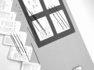
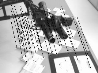
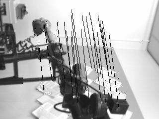
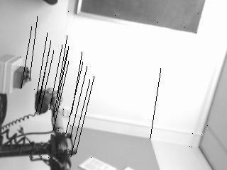
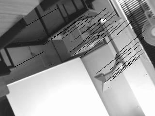
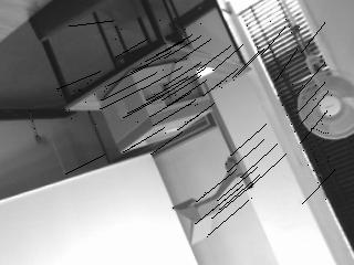
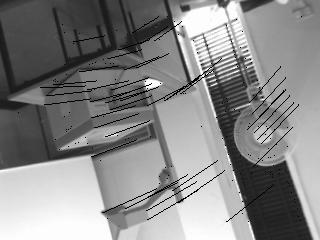
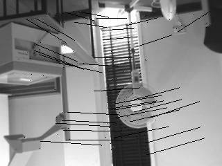
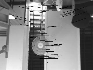
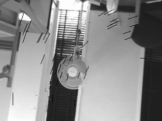
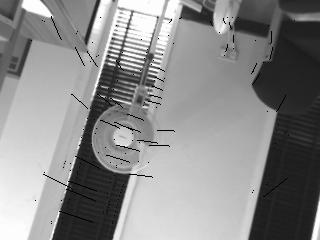
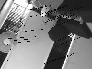
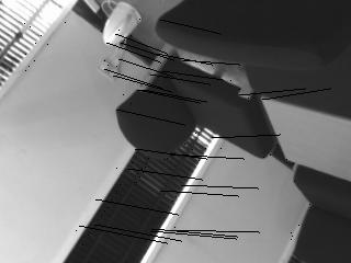
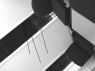
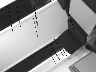
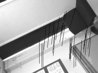
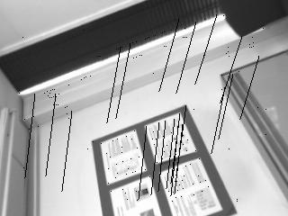
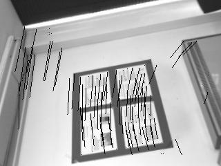
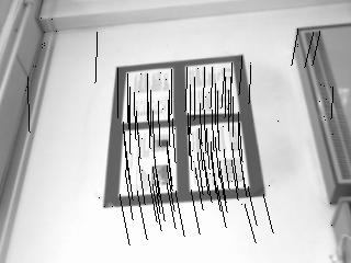
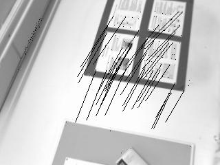
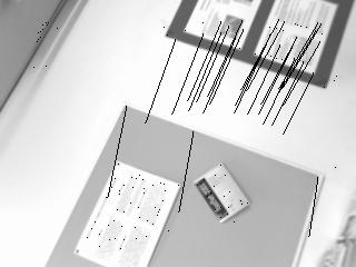
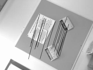
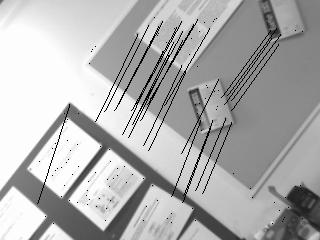
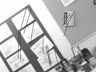
87 CHAPTER 5. CAMERA MOTION ESTIMATION 72 Figure 5.4: The complete seminar room sequence with arbitrary motion, sampled with 1.5fps. The movement of consistent correspondences is marked with black lines.

88 CHAPTER 5. CAMERA MOTION ESTIMATION 73 Number of Points (a) Rank Correlation Usable Corners Initial Corresp. Consistent Corresp. Corresp. for Calc Sequence Number of Stereo View Number of Points (b) LoG/SAD Correlation Usable Corners Initial Corresp. Consistent Corresp. Corresp. for Calc. Number of Points (c) Rank with Big Correspondence Set Usable Corners Initial Corresp. Consistent Corresp. Corresp. for Calc Sequence Number of Stereo View Sequence Number of Stereo View Figure 5.5: The number of corners and correspondences in the seminar room sequence with arbitrary motion using Rank (a), LoG/SAD (b) and a large initial correspondences set (c). the first view (Section 5.3.2). Only correspondences, which are found both ways are maintained. A large set of initial correspondences can be created by adding correspondences that are found in both directions. This set contains much more outliers. Figure 5.5c shows the robustness of creating a consistent set of correspondences even in this case. It can be seen that the number of initial correspondences is now higher than the number of corners in a view, due to the creation of the superset of correspondences. Nevertheless, the curve of consistent correspondences looks very similar to the one in Figure 5.5a. The mean number of consistent correspondences increased from 38 to 42 and the minimum from 8 to 9. This example shows that the creation of the consistent correspondence set is very robust, even in the presence of a much higher number of outliers. Furthermore, this example seems to show that the correspondence check is obsolete. However, the creation of a set of 2 consistent correspondences requires O n c n steps (Section 5.3.3), while the correspondence check only involves O n steps. Therefore, it is computationally more advantageous to use the correspondence check to reduce the number of initial correspondences, before the consistent correspondence set is created. This evaluation has shown that the choice of using Rank correlation with a correspondence check performs well to establish initial correspondences. Additionally, the robustness of outlier

89 CHAPTER 5. CAMERA MOTION ESTIMATION 74 detection and the creation of a set of consistent correspondences has been demonstrated on a set with much more outliers than inliers. The correct determination of consistent correspondences is an important prerequisite for calculating camera motion accurately Accuracy of Motion Calculation The accuracy of the SCS method was determined on 5 stereo image sequences. Some images of all sequences are shown in Figure 5.6. All sequences are closed, which means that the last view overlaps with the first one. This permits the determination of the overall error of the sequence elegantly, by calculating motion from the last to the first view. The rotation and translation difference between the first view and the revisited first view represents the overall error. This error only depends on the performance of motion estimation and does not include evaluation errors. The sequences are taken in 3 different indoor and 1 outdoor environment. All sequences were sampled with 8fps (frames per second), which results in a moderate camera movement between consecutive views. The main movement in 4 sequences is in a circle parallel to the ground, with some forward, backward and sideward movement. Additionally, the sequence with arbitrary three-dimensional camera movement in the seminar room (Figure 5.4, but sampled with 8fps) was used. All camera movements were performed by hand and include considerable amount of jitter. The challenges from the arbitrary camera movement and the complexity of environments can be best judged from video clips, which are attached on CD. Table 5.1 gives more details about the sequences. It lists the number of views from which motion was calculated, the mean number of correspondences and the sum of all individual camera rotations and translations as determined by the best performing calculation (i.e. with lowest error). Name of Sequence Sampling Used Consist. Corresp. Abs. Dist. Abs. Rot. [fps] Views Corresp. for Calc. [mm] [deg] Seminar room Seminar room (arb.) Living room Bedroom Garden Table 5.1: Description of 5 closed stereo image sequences, which were used in the evaluation. The rotation and translation errors of motion estimation of all sequences is shown in Figure 5.7. Motion was calculated with 4 different error models, with and without rejection of suspicious correspondences during calculation as described in Section First, the performance of different error models while performing rejection of suspicious correspondences during calculation is discussed (i.e. dark bars). Figure 5.7 shows that the spherical error model performs on all sequences worst and the image based model best. The performance of the ellipsoid error model is usually almost as good as the performance of the image based error model. It was expected that

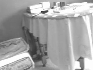
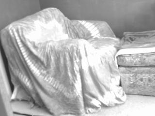
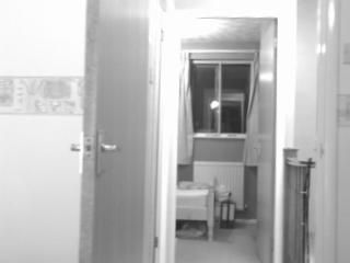
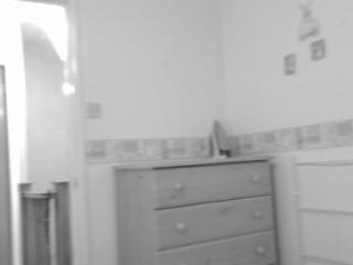
90 CHAPTER 5. CAMERA MOTION ESTIMATION 75 (a) Seminar Room (b) Seminar Room (arb.) (c) Living Room (d) Bedroom (e) Garden Figure 5.6: Some images of 5 closed stereo image sequences, which were used in the evaluation.

91 CHAPTER 5. CAMERA MOTION ESTIMATION 76 Absolute Rotation Error [deg] (a) Absolute Rotation Error Without Rejection With Rejection Spherical: Sp Ellipsoid: El Ellipsoid with Comp.: EC Image Based: IB Sp El EC IB Sp El EC IB Sp El EC IB Sp El EC IB Sp El EC IB Seminar room Seminar room (arb.) Living room Bedroom Garden Absolute Translation Error [mm] (a) Absolute Translation Error Without Rejection With Rejection Spherical: Sp Ellipsoid: El Ellipsoid with Comp.: EC Image Based: IB Sp El EC IB Sp El EC IB Sp El EC IB Sp El EC IB Sp El EC IB Seminar room Seminar room (arb.) Living room Bedroom Garden Figure 5.7: Motion error of all sequences with different error models, with and without rejection of suspicious correspondences during calculation. drift compensation improves the ellipsoid error model. However, drift compensation does not cause a reduction of ellipsoid errors. It seems that the approximation of the image based error in both image planes with equal parts of the ellipsoid error (Section 4.4.4) is either wrong or biased. The effect of the error model on the camera path is shown for the seminar room sequence in Figure 5.8. The camera position and orientation on the path is marked for every 5th view. Camera motion was determined without any restriction on the three-dimensional movement and orientation of the camera. However, only the two main dimensions of the camera movement are shown for visualisation reasons. The spherical error model underestimates rotation completely (Figure 5.8a). The ellipsoid error model performs much better, but the first and last camera positions do not match (Figure 5.8b). Drift compensation does not seem to have any effect (Figure 5.8c). Finally, the image based error model performs nearly perfect (Figure 5.8d). Rejection of suspicious correspondences during calculation reduces errors considerably, especially with the ellipsoid and image based error model (comparison of neighbouring dark and light bars in Figure 5.7). A comparison of column 4 and 5 in Table 5.1 reveals that less than 4% of consistent correspondences are rejected. Thus, the rejection phase during calculation identifies and removes erroneous correspondences very effectively.

92 CHAPTER 5. CAMERA MOTION ESTIMATION Camera (a) Spherical Error Model Camera Path 500 Camera (b) Ellipsoid Error Model Camera Path 0 0 y [mm] -500 y [mm] x [mm] x [mm] 500 (c) Ellipsoid Error Model with Compensation Camera Camera Path 500 Camera (d) Image Based Error Model Camera Path 0 0 y [mm] -500 y [mm] x [mm] x [mm] Figure 5.8: Camera path with different error models on the seminar room sequence. Every 5th camera position and orientation is shown with v-shaped boundaries of the horizontal field of view. The number of correspondences from which motion is calculated is important for the accuracy of motion calculation. Obviously, the number of correspondences depends on the number of corners, which is higher in highly textured environments. The mean number of correspondences from which motion is calculated exceeds 100 in the living room and garden sequence. Figure 5.7 shows that both sequences have very low motion errors. The bedroom sequence has the lowest mean number of correspondences and performs worst, as expected. The effect of arbitrary camera movements on motion estimation can be seen in Figure 5.7 as well. The motion error of the seminar room sequence with arbitrary motion (Figure 5.4) is only slightly higher than in other sequences. It has to be considered, that this sequence is longer and camera rotation and translation is larger than that of other sequences as shown in Table 5.1. Thus, a slightly higher error is normal and does not depend on the kind of motion. The bedroom sequence does not only perform worst due to the relatively low number of correspondences. It is the only sequence in which a part of the motion error is caused by a failure of finding the correct correspondences between two views. Figure 5.9 shows the problematic views. Correspondences (i.e. marked with black lines) are found exclusively on a stripe of repetitive texture on the wall. Unfortunately, the wrong parts of the texture were matched. Outlier detection

93 CHAPTER 5. CAMERA MOTION ESTIMATION 78 (a) Previous and Current Image (b) Previous and Current Image with correspondences marked Figure 5.9: Problematic, consecutive images of the bedroom sequence (a), where repetitive texture leads to wrong correspondences, which are marked with black lines (b). failed to detect the mismatch, because the spatial relationship between features is maintained. This mismatch causes a small jump in camera position, which is the main cause of the high motion error in this sequence. This kind of error can only occur under special conditions and is therefore very rare. It was only encountered once during all tests, which involved thousands of stereo images. Hence, the best performance is with the image based and ellipsoid error model, with rejection of suspicious correspondences during calculation. The performance of motion estimation is independent of the kind of camera movement and environment. However, highly textured environments perform better, due to a higher number of correspondences. Generally, the motion error increases with the amount of absolute rotation and translation and decreases with higher numbers of correspondences. All evaluations in this Section were performed on sequences, which were sampled with 8fps. A change of the frame rate causes higher or lower differences in consecutive views, which influences the accuracy of motion Dependency of Accuracy on Frame Rate The effect of changing the frame rate of the seminar room sequence with arbitrary camera motion (Figure 5.4) is shown in Figure Smooth Bezier approximations of the data is overlayed in the graph, to show the main tendency in the data. Motion was calculated between 1.5fps and 25fps

94 CHAPTER 5. CAMERA MOTION ESTIMATION 79 which corresponds to sampling the 30s sequence using between 45 to 750 views. The difference between some consecutive images becomes too high to establish correspondences below 1.5fps. The graph confirms that the image based error model always performs better than the ellipsoid error model. Again, drift compensation does not show improvements of the ellipsoid error model. The performance of the image based error model seems almost independent of the frame rate, with slight improvements at higher frame rates. This is surprising as the use of more images should introduce more errors. However, a higher frame rate means also that consecutive views are less different, which results in a higher number of correspondences and therefore in more accurate motion estimation. It seems that both effects almost compensate each other. Absolute Rotation Error [deg] (a) Absolute Rotation Error Ellipsoid Model Ellipsoid Model with Comp. Image Based Model Sampling [fps] Absolute Translation Error [mm] (b) Absolute Translation Error Ellipsoid Model Ellipsoid Model with Comp. Image Based Model Sampling [fps] Figure 5.10: Motion error of 30s seminar sequence with arbitrary camera motion in dependency of the frame rate. Smooth Bezier approximations of the data is overlayed to show main tendency. In contrast, the ellipsoid error model performs worse at higher frame rates. This can be explained by the slight bias in the ellipsoid error calculation as discussed in Section This bias is stronger with lower changes in position of the camera of consecutive views, which is the case with higher frame rates. The bias is minimised with higher changes in position, which corresponds to lower frame rates. This constant bias cannot be compensated by higher number of correspondences. The optimum of the ellipsoid error model in this sequence is between 4fps and 9fps. Olsen et al. [120] compensate the constant bias of the ellipsoid error model, by tracking feature positions through several images. The image based and ellipsoid error model have in common that very low frame rates increases errors, because the number of correspondences is reduced due to higher differences in consecutive views. Small errors in the position of correspondences have a stronger effect with lower number of correspondences. If the frame rate is too low, then establishing correspondences fails, and the method breaks down. The lowest possible frame rate depends obviously on the amount of texture in the environment and on the speed of camera movements, which are determined by the application. The highest frame rate is limited by the hardware. Typical cameras produce images at 25fps. However, the computational effort to calculate the disparity image and perform motion estimation

95 CHAPTER 5. CAMERA MOTION ESTIMATION 80 reduces this theoretical limit Speed of Camera Motion Estimation The speed of the SCS method is critical for real time applications, especially because other computational modules like the stereo algorithm are performed concurrently. The SCS method has been implemented in C and optimised. Additionally, time critical parts of corner detection and correlation have been implemented with SIMD assembler instructions. Figure 5.11 gives an overview of all phases of the SCS method on the seminar room sequence with arbitrary camera movements (Figure 5.4). Time [ms] Speed of Motion Estimation on Seminar Room Seq. with Arbitrary Motion Corner Det. (158) Init. Corresp. (105) Consist. Corresp. (79) Calc. (Spherical) (76) Athlon 1.2GHz Pentium 4 2GHz Opt. Calc. (Ellipsoid) Opt. Calc. (Ellipsoid Comp.) Opt. Calc. (Image Based) Figure 5.11: Speed of individual components of the SCS method on the seminar sequence with arbitrary camera movements. The mean number of corners and correspondences is given in brackets. The speed of corner detection depends exclusively on the image size, which was pixel. The determination of initial correspondences involves O nh 2 steps, with n h corners according to Section A set of consistent correspondences is established in O n c ni 2 steps as discussed in However, the steps are relatively simple and can be performed fast. The calculation of motion depends also on n c as well as on the data itself. The spherical error model is very fast, because it can be calculated directly. The ellipsoid error model is also fast and therefore suitable for real time use. The image based error model is relatively slow, due to the nested numerical calculation, as discussed in Section Generally, processing speed decreases with more correspondences, which leads to higher camera motion until the next images can be processed. However, higher image differences result in less correspondences, which increases processing speed again. This behaviour is advantageous for real time applications. The use of rectification, MWMF stereo algorithm (including all methods, but excluding interpolation) and the SCS method with the image based error model results in- 6 3 frames/s on the Athlon and frames/s on the Pentium 4 configuration. If the ellipsoid error model is used instead of the image based model, then the frame rate increases to- 9 4 frames/s on the Athlon and

96 CHAPTER 5. CAMERA MOTION ESTIMATION frames/s on the Pentium 4 configuration. This data suggests that the image based error model can be used if high motion accuracy is required and fast computer hardware is available. Otherwise, the ellipsoid error model should be used. 5.5 Conclusion The SCS method for the estimation of stereo camera motion has been presented in Section 5.3. The robustness and reliability of the technique is due to an accurate determination of consistent correspondences. This has been achieved by using the experience from stereo correlation and adopting certain stereo correlation techniques (Section 5.3.2). Additionally, rigidity constraints are exploited to their full potential by using accurate error characteristics of feature positions (Section 5.3.3). This results in an almost error free correspondence set, even if consecutive views are highly different, due to a low frame rate. It has been identified in Section 5.4 that motion calculation with the image based error model performs best, but it requires fast computer hardware for real time performance. However, a fast and good approximation can be achieved using the ellipsoid error model. The performance of motion estimation does not depend on the kind of environment. However, more texture increases the number of correspondences, which makes motion estimation more accurate. Motion is calculated between consecutive views, without predictions of feature positions or other sensors in contrast to most other techniques. The SCS method works with arbitrary camera movements, which has been shown in Section The presented technique even permits to calculate camera motion reliably between chronologically unrelated views, in contrast to other methods. This makes the SCS method suitable for a wide range of applications, including those that involve multiple stereo cameras. It has been shown that the method works usually very well. However, there are four areas which require consideration, depending on the specific application. The method depends on the three-dimensional localisation of features through stereo vision. The currently used stereo camera permits accurate localisations of features between 1m and 10m, which is suitable for indoor environments. Features outside this range cannot be used for motion estimation. This distance range depends on the stereo camera (i.e. baseline, field of view, and resolution) as well as the disparity search range, which have to be adapted, depending on the application. The approximation of the image based error model with the ellipsoid error model is limited. This is a problem for applications that require the accuracy of the image based error model, but do not have the computational power to use it. The proposed drift compensation does not improve the approximation as expected. Probably because the approximation of the image based error in both image planes with equal parts of the ellipsoid error is either wrong or

97 CHAPTER 5. CAMERA MOTION ESTIMATION 82 biased. Future research should focus on finding a closed form solution to calculate the image based error fast or finding a better approximation of it. The method breaks down, if motion between consecutive views is too fast or if there is not enough texture in overlapping parts of the views available to identify correspondences. This problem can partly be addressed with higher frame rates. However, breakdowns should be anticipated. A possible strategy for recovery could infer the camera motion from past movements as a rough estimates. Despite all efforts to increase accuracy, there will always be a growing motion error, due to accumulation of small errors or breakdowns. This is especially a problem for long sequences, which revisit the same environment. The SCS method offers the unique feature to calculate motion between any overlapping views despite their chronological order. Thus, motion can be calculated to past views as well, if an overlap is likely. If motion calculation to a past view is successful, then the camera position and orientation will be derived from this relationship and the difference can be propagated backwards in the sequence. In this way, the camera position would never get out of synchronisation with past positions and the error growth can be stopped. The recovery of the three-dimensional structure of a scene part from one stereo image and their relation through camera motion estimation allows to describe a complete scene with a collection of stereo views. The only requirement is a calibrated stereo camera that moves arbitrarily through a scene. The collected stereo views implicitly describe the complete three-dimensional scene structure and texture. This implicit model is the bases for methods that create visual representations like map overview or virtual images from certain viewpoints.

98 6 Map Building 6.1 Introduction The three-dimensional structure and texture of a scene can be represented with a collection of stereo views. Each individual stereo view describes a part of the scene. The relation between all stereo views is recovered by determining the motion of the camera (Chapter 5). The representation with stereo views is implicit, as it can not be visualised directly. However, different representations can be created from it. The aim of this Chapter is the creation of a two-dimensional map of the environment from a stereo camera under arbitrary three-dimensional motion. An occupancy grid is used to represent the map. Occupancy grids divide the environment into equally sized cells that can either be occupied by obstacles or empty. The map is intended as an overview for the operator of a teleoperated mobile robot (Section 1.2). It should allow to identify obstacles and free space around the robot, which travels through an unknown environment. Section 6.2 discusses literature about map building and identifies that almost all published approaches deal only with two-dimensionally moving sensors. Section 6.3 presents a new approach for creating two-dimensional maps from stereo images of a camera that moves arbitrarily in three-dimensions. Maps are created memory efficiently and incrementally with the arrival of new stereo and motion data in real time. An evaluation is made in Section 6.4. The presented method has been published previously [64]. 6.2 Related Literature Mapping can be performed using data from different kinds of sensors. Ultrasonic sensors are inaccurate, but cheap and therefore often available in robotics applications and used for mapping [33, 49, 50, 84, 121]. Laser scanners are much more accurate and therefore more suitable for exact mapping [56, 57, 145, 151]. Stereo vision is less accurate than laser scanners and requires computational power. However, it provides not only range, but also intensities or colour information. Mapping has been performed from three-dimensional lines, which were detected by feature-based stereo vision [5, 161]. Other approaches use scan-line stereo vision [87, 116], which measures distances in a plane like two-dimensional laser scanners. Dense stereo vision has also been used 83

99 CHAPTER 6. MAP BUILDING 84 [31, 111, 112, 146]. Furthermore, combinations of different sensors like ultrasonic and vision [24, 86, 104] have been utilised to compensate weaknesses of different sensors. DeSouza and Kak [26] surveyed 20 years of research in the field of vision based navigation for mobile robots. The sensor data can be used to create either topological [24, 86] or geometric maps with a high precision [56, 57, 145]. This research concentrates on geometric maps, which can be easily communicated to an operator. Two-dimensional maps can be represented with features like lines [50], circles [151] or splines [31]. Three-dimensional maps can utilise lines from feature-based stereo vision [5, 161] or build a triangular mesh from a three-dimensional laser scanners or dense stereo vision [67]. Elfes and Moravec [34] introduced occupancy grids, which divide the environment into equal cells. The state of each cell (i.e. occupied or empty) is updated from sensor data. Two-dimensional occupancy grids have been a popular choice for inaccurate ultrasonic sensors [33, 49, 84, 121], but also for scan-line stereo vision [116]. Furthermore, their power to explicitly model sensor uncertainties allows the combination of ultrasonic sensors and scan-line stereo vision [104], which have very different characteristics. A natural extension of two-dimensional occupancy grids are three-dimensional grids with cubic cells. Moravec [111, 112] and Tirumalai et al. [146] describe three-dimensional occupancy grids, which are updated by dense stereo vision. Traditionally, occupancy grids and sensors are modelled statistically [33, 34, 104, 111, 112]. However, the use of probability theory has been criticised for several reasons. Firstly, a single probability does not distinguish between unknown and uncertain occupancy (i.e. it models the probability of occupancy and is initialised with 50%, which means unknown, but also uncertain occupancy). Thus, it cannot be determined whether an area has not been scanned at all (e.g. due to occlusion) or the sensor data was unreliable. The Dempster-Shafer theory [25, 131] has been used to tackle this particular problem [146]. Secondly, the violation of strong assumptions can lead to large errors. The assumption of independence of different scans is usually violated for a slowly moving robot. Enforcing this independence artificially improves map building [84]. Finally, there are other implicit assumption like the even distribution of occupied cells. However, occupied cells usually appear clustered in natural scenes [49]. Gambino et al. [49] compared probability theory, Dempster-Shafer theory and fuzzy logic for map building from ultrasonic sensors. They show that probability theory and Dempster-Shafer theory are sensitive to erroneous measurements, which resulted in serious errors in the maps. This was attributed to unrealistic simplifying assumptions of these theories in order to obtain a computationally feasible algorithm. It was shown that fuzzy logic produced more accurate maps in the presence of conflicting data, which was attributed to less constraining hypotheses. There is more freedom in fuzzy logic to chose the right operators to tackle specific problems. The fuzzy logic method of Gambino et al. has been improved by Oriolo et al. [121] by taking dynamic environments into account. Almost all of the discussed methods constrain the sensor movement to two dimensions parallel to the ground plane. This is even true for most methods, which produce three-dimensional maps. Exceptions are Huber et al. [67] who registered range scans from a sensor (i.e. dense stereo vision

100 CHAPTER 6. MAP BUILDING 85 or three-dimensional laser scanner) under unknown motion. However, the approach is unsuitable for real time purposes, because it is computationally too expensive. Tirumalai et al. [146] update a three-dimensional occupancy grid from dense stereo views from possibly arbitrary positions and orientations. However, three-dimensional occupancy grids require huge amounts of memory and considerable computational power. It is possibly to model occupancy grids with octrees [156] to save memory, but this increases accessing time for individual cells. The aim of the target application in this work is to create a two-dimensional map from an arbitrary moving stereo camera in real time (Section 1.2). Section 4.4 showed that the reconstruction error of stereo vision depends heavily on the distance between the camera and reconstructed point. Occupancy grids have been chosen, because they can easily merge data with very different error characteristics [104]. The argumentation for fuzzy logic [49, 121] is followed and the method from Oriolo et al. [121] used as a basis. However, modifications are required as dense stereo vision is modelled very differently to ultrasonic sensors. Furthermore, arbitrary camera positions and orientations need to be supported. This requires an extension of the method to three dimensions, but without using memory and computing intensive full three-dimensional occupancy grids. The presented mapping method has been published [64]. 6.3 A Fuzzy Logic based Layered Occupancy Grid Overview Mapping is based on the MWMF stereo algorithm (Section 3.4) and the SCS motion estimation method (Section 5.3). Figure 6.1 gives an overview over the Fuzzy logic based Layered Occupancy Grid (FLOG) mapping method. Set of 2D/3D points from previous image Previous mapped position, orientation Previous 3D grid Rect. left image Camera Motion Estimation Position, Orientation Position or orient. different enough? y Grid update Rect. right image Disparity image Stereo correlation Disparity image n Skip view Updated 3D grid Visual map creation Visual 2D map Figure 6.1: Overview over the FLOG mapping method. The disparity image and corresponding position and orientation of the camera are used to incrementally update a layered three-dimensional occupancy grid. However, only views, which are

101 CHAPTER 6. MAP BUILDING 86 different enough to the last mapped view are used for mapping. The geometry of the grid is derived in Section Selection of views and updating of the state of grid cells using fuzzy logic is discussed in The three-dimensional occupancy grid is used as an internal representation of the environment. Section discusses the transformation of the occupancy grid into a two-dimensional map, for visualisation. Appendix A.5 describes a memory efficient implementation of the occupancy grid, which is important for the target application Geometry of the Occupancy Grid The easiest way to use stereo vision for map building is by reducing its data immediately from three to two dimensions, either by using only one scan-line or by constructing a scan-line by selecting the closest point in every column of the disparity image [116]. However, this restricts possible movements of the camera to two dimensions as the scan-line is expected to represent measurements parallel to the ground. Furthermore, the latter variant only works due to the fact that stereo vision cannot detect distances on objects without texture and the ground is usually untextured. Otherwise, the closest point on the ground would be constantly picked up as obstacle. This is clearly a problem if the ground is textured. Modelling stereo vision three-dimensionally, leads to memory consuming three-dimensional occupancy grids with cubes as cells [111, 112, 146]. However, the vertical resolution (i.e. height above ground) can often be chosen to be much lower than in the other two dimensions, which saves memory. Figure 6.2 depicts this case. Grid cells are modelled as boxes. This will be called a layered occupancy grid, to distinguish it from three-dimensional grids with cubic cells. The height of each layer is application dependent. Applications that do not require explicit knowledge about the height of obstacles may choose only one big layer. Ellipsoid of image based error Measured distance Reconstructed ray of light Optical centre of left camera Occupancy grid cell Figure 6.2: The layered occupancy grid. The disadvantage of introducing an asymmetry in the size of cells is that the orientation of the grid needs to be aligned with the environment. The transformation R k, T k of the kth camera position to the occupancy grid depends on the transformation R 1, T 1 between the first camera position and

102 CHAPTER 6. MAP BUILDING 87 the occupancy grid as shown in equation (5.5) in Section R 1, T 1 can be defined by manually aligning the first camera position with the occupancy grid (e.g. optical axis of the first camera is parallel to the ground and the horizon is horizontal in the image). Alternatively, it could be assumed that the ground plane is parallel to the main movement of the camera (i.e. best fitting plane through all camera positions) to define R 1, T 1. Unfortunately, this prevents incremental map creation as the ground plane cannot be pre-determined. Therefore, the first possibility (i.e. manually aligning the first camera position with the environment) has been used throughout this study. The camera position R k, T k is used to calculate the position of reconstructed points in the occupancy grid as shown in Figure 6.2. Reconstruction is performed from the disparity image as discussed in Section 4.3. It has been shown in Section that the error distribution around a reconstructed point has a very long ellipsoid shape whose size depends on the image based error. A grid cell is supposed to be partly occupied if the ellipsoid intersects with it. Furthermore, the conically shaped space between the ellipsoid and the optical centre is presumed to be unoccupied. The cone is labelled as a reconstructed ray of light in Figure 6.2. Ultrasonic sensors are commonly used to update occupancy grids. These sensors emit very wide beams. Each cell that is inside such a beam can be considered completely empty. In contrast, the width of the ellipsoid uncertainty around the reconstructed point and the corresponding conic ray are typically much smaller than grid cells (unless cells are very small, which would be very memory consuming). This requires different considerations for updating the occupancy grid Updating of the Occupancy Grid The ellipsoid error in the position of a reconstructed point P i is far higher in the direction of the reconstructed ray of light than in all other directions. Therefore, the error is modelled onedimensionally with the propagated distance error l c, which is calculated with equation (4.24) in Section For camera motion estimation, the image based error was set to p 0 1 (Section 5.3.3). This same value is used for mapping. The assumed Gaussian distribution around P i is approximated by a triangular function using 3 times l c as maximum error. These simplifications of the full ellipsoid error distribution are chosen to speed up computations, since the corresponding calculations have to be done hundreds of thousands of times per second. Additionally, the resolution of the disparity image can be reduced to increase speed if required. For camera motion estimation (Section 5.3.1), disparities below 4 pixel (i.e. 10m on the used cameras) have not been used, due to increased distance error. For the same reason, reconstructed rays will only be traversed up to this distance in the occupancy grid. The membership functions (appendix A.4) for emptiness and occupancy for reconstructed point P i can be formalised with parameter r as distance from the optical centre (i.e. positive in the direction of sight) as shown in equation (6.1).

103 %& === %& === CHAPTER 6. MAP BUILDING 88 µ Ei 1 if r #=== r" 0 and r, l c 3 l c, l c r 3 l c if r" l c 3 l c and r, l c, 0 otherwise. µ Oi l r #=== 1 c r 3 l c if r" l c 3 l c and r, l c, l 1 r c 3 l c if r" l c and r, l c 3 l c, 0 otherwise. (6.1a) (6.1b) The membership functions are visualised in Figure 6.3. These functions are mapped into the occupancy grid by considering only cells C through which the reconstructed ray to point P i passes. The parameter r is determined for each cell as the point on the ray that is closest to the middle of the cell. Membership Membership 1 Ei 0 0 l c 3 l c l c Distance 1 O i 0 0 Distance l c 3 l c lc l c 3 l c Figure 6.3: Membership functions for emptiness E i and occupancy O i for point P i. The sensor data is directly fused into the global occupancy grid in contrast to the approach of Oriolo et al. [121]. Oriolo et al. demonstrated the advantage of using an averaging calculation instead of a union operator so that memberships of cells do not only increase but also decrease. This is important to compensate errors with new data and to account for partly dynamic environments. Therefore, this choice has been assimilated. The memberships to the empty (µ E C ) and occupied fuzzy set (µ O C ) of cell C are updated with equation (6.2) if the ray to P i passes through the cell. µ>e C N C 1 µ E C µ Ei C N C µ>o (6.2a) C N C 1 µ O C µ Oi C (6.2b) N C The number of rays through cell C is counted in N C. An advantage of this formulation as Oriolo et al. [121] point out is that N C can be limited using a maximum threshold N t. This effectively limits the influence of past measurements and allows updating the map quickly to changes in the environment from new data. An extension for stereo vision is the calculation of the membership of cell C to the confidence fuzzy set K using the number of measurements in a cell as shown in equation (6.3).

104 CHAPTER 6. MAP BUILDING 89 µ K C N C N K (6.3) The parameter N K represents the number of rays that are required to give full confidence in the correctness of µ E and µ O. This formulation of confidence coincides nicely with the error characteristics of stereo vision. The number of rays that can pass through a cell increases with the square of decreasing distance of the cell from the camera. The same is true for the accuracy, as the reconstruction error decreases with the square of decreasing distance according to Section Thus, less accurate data is treated with proportionally less confidence. For this study, N K has been chosen as the number of rays that pass through a fully visible cell observed at close distance, i.e. 1m. The threshold N t has been set to 3N K. There are two issues which require consideration. Firstly, the calculations of emptiness, occupancy and confidence are only correct for fully visible cells. Partly visible cells introduce errors, because the measurements of a part of a cell do not necessarily reflect measurements of the whole cell. Smaller cells are less likely to be partly visible, but they lead to an increased memory consumption. The main importance of this issue is to choose the height of layers so that they are not too big, i.e. a camera that is close to a cell should still be able to observe the cell completely. Secondly, multiple stereo images from the same camera position do not contain additional information, but often the same systematic errors, e.g. increased size of objects due to object border problems. Therefore, as a heuristic, new views are only added if the translation between the last added view is at least 4 grid cells or if the rotation is more than half of the field of view (i.e. 21 for the current cameras). It is important to note the change in the meaning of cell memberships using different sensors. For ultrasonic sensors with a beam that is much larger than cells, the memberships represent the belief that a cell is completely empty or partly occupied. In stereo vision the memberships reflect the ratio to which a cell is empty or occupied. This has an impact on processing these values for the creation of visual maps Creation of Visual Maps One strength of the fuzzy logic approach is that maps can be defined for different purposes. Oriolo et al. [121] define a map that is safe for motion and one that is safe for planning. The difference is the treatment of undetermined areas. The former map treats them as being occupied, while the latter one as being empty. For the visualisation of the map to the operator, undetermined areas will be treated as if they are empty. Calculation of the visual map is derived from the approach of Oriolo et al. Differences are that it does not make sense to calculate a measure of ambiguity for cells, since cells that are partly empty and partly occupied are explicitly modelled. Furthermore, the measure

105 CHAPTER 6. MAP BUILDING 90 of confidence (6.3) is new. Finally, multiple layers of two-dimensional grids are used, that have to be fused. The map value M k is calculated for each layer k separately. A measure of indeterminateness I is calculated as not empty and not occupied. A cell, which is safe for planning must be empty and not occupied or its value must be indetermined, i.e. E? Ō A@ I. The complement of this value gives the degree to which a cell is unsafe (i.e. inhabited by obstacles). The map value M k is defined by the intersection of unsafeness and confidence in the correctness of the measurements. Thus, unsafe areas are rated by confidence for visualisation. The translation of this description to fuzzy logic results in equation (6.4), which uses standard fuzzy logic operators (appendix A.4). M k E? Ō B@ I? K I Ē? Ō (6.4) Layers could be represented using different colours to visualise different heights. However, for this study, they are all combined into a two-dimensional map according to equation (6.5). km k (6.5) The resulting value M, which is between 0 and 1 is mapped to intensities between white and black for visualisation. It is important to note that the fusion of several layers is superior to using only one layer, because increasing the height of cells introduces errors if cells are often only partly observed, as discussed at the end of Section All calculations are simple, which supports fast computations. Another important issue for real time applications is to organise occupancy grids internally in a memory efficient way. Appendix A.5 shows a memory efficient way to implement occupancy grids. 6.4 Evaluation of Map Building Mapping of a Simple Scene The characteristics of the described mapping method are demonstrated on a simple scene with two boxes as shown in Figure 6.4a. The stereo camera was circled in 32 steps around the centre of the big box ( mm). The camera position and orientation was determined exclusively from consecutive stereo views with the SCS motion estimation method from Section 5.3 using the image based error model. Only one map layer, which covers the height of the bigger box was used. The size of each grid cell was set to mm. Thus, the space over and under the box (e.g. the table) is excluded from the map. Mapping was performed once from a close distance of 1.1m and once from a moderate distance

106 CHAPTER 6. MAP BUILDING 91 (a) Setup of Experiment from 1.1m Distance (b) Mapping of Boxes from 1.6m 2.0m Distance Considered height range Stereo camera Figure 6.4: Mapping of two simple objects. between 1.6m and 2.0m as shown in Figure 6.4b. The individual camera positions and the camera path appears as ring around the boxes. The overall motion error was just 1 3 and 12mm for the distance at 1.1m and 2 6 and 63mm at the distance between 1.6m and 2.0m. It can be seen from both maps that two sides of the smaller box ( mm) are very weak, which is due to obstruction from the bigger box. It is interesting how the sides of the boxes are represented thicker when the distance of the camera increases. This is a direct result of equation (4.24), which is used in Section to create the membership functions (i.e. the uncertainty in distance l c increases with the square of the distance l c to an obstacle). Thus, grid cells around occupied cells are also declared as possibly occupied in absence of more accurate close range data. Clearly, mapping works well in the case of a simple scene Mapping of Real Scenes Mapping was evaluated on the closed stereo sequences from Section and two longer sequences, which cover several rooms. One of the closed sequences is shown in Figure 5.4 in Section However, the complexity of the camera movements and environments of all sequences can be best judged from video clips, which are attached on CD. The MWMF stereo method from Section 3.4 was used to calculate the disparity image. General matching errors would introduce false objects in the map. The reduction of these errors with the Correlation Function Error Filter (Section 3.4.3) and the Segment Filter (Section 3.4.5) are important for mapping from disparity images. Murray and Little [116] made the same observation from their mapping method. Generally, mapping benefits from using only very reliable disparities. Therefore, it is not advantageous to perform interpolation between segments with the simple method from Section However, interpolation can be performed within segments, which is much more reliable. Camera motion estimation was performed purely from consecutive stereo views with the SCS method from Section 5.3. All sequences were sampled with 8fps and the effect of the ellipsoid and image based error model of motion estimation are compared. The size of occupancy grid cells was set for all sequences to

107 CHAPTER 6. MAP BUILDING mm with 3 layers, which covers a height range of 2.1m. The image based error p was set to 0.1pixel as discussed in Section Mapping can be performed with all valid disparity values of the disparity image, which is a huge amount of data. For this study, the vertical resolution of the disparity image was reduced by using every second row of data to increase the speed of mapping. Figure 6.5 shows fours stages of a map, which was created from the seminar room sequence with arbitrary camera motion. The camera is depicted in the middle of the maps with two lines, which mark the horizontal boundaries of the field of view of the camera. These lines almost match each other in the left map, which means that the camera is on its side. This example shows that the method can perform incremental mapping using information from arbitrary camera positions and orientations. Figure 6.5: Four stages of an incrementally created map using the seminar room sequence with arbitrary camera motion (Figure 5.4 in Section 5.4.1). The results of mapping of the 5 stereo image sequences from Section are shown in Figure 6.6. The left column shows manually created simplified outline maps of individual environments (Figure 6.6a). Clearly, this level of abstraction cannot be expected from a method that works on the pixel level without any reasoning. It is also important to note that the outline maps are simplified as they do not show small details like door handles, curtains, etc. However, these details will be picked up by stereo vision. Furthermore, some parts of furniture are never seen in any stereo image, due to occlusions or because they were permanently outside the field of view due to the general camera movement. Furniture, which is completely unseen, is marked with dashed lines in the outline maps. All of these issues must be considered by comparing the outline and the automatically created maps. The middle column (Figure 6.6b) shows maps that were automatically generated using the ellipsoid error model for motion estimation. The right column (Figure 6.6c) shows the result using the image based error model. The camera path and the last position and orientation of the camera is marked. Differences between both error models can be best seen on the seminar room map with arbitrary camera movement and the bedroom map. In both maps, the upper part is not properly aligned when the camera comes back to that position. The performance of the image based error model is better. Nevertheless, the differences are minor. The suggestion from Section 5.5 to syn-

108 LLLKKK JJJIII CHAPTER 6. MAP BUILDING 93 (a) Simplified Outline Maps (b) Maps (Ellipsoid Error Model) (c) Maps (Image Based Model) Seminar Room 5.36m 5.64m Seminar Room (Arbitrary Camera Movement) 5.36m 5.64m Living Room 3.7m 3.7m Bedroom 3.7m 2.6m CDEE EE FF FF GH GH GH GH GH GH GH GH GH GH NNMMMNO OP Garden 3.9m 5.6m Figure 6.6: Mapping of closed sequences (from Section 5.4.2) with different error models for motion calculation. Furniture, which is marked with dashed lines is not seen in any camera image.

109 CHAPTER 6. MAP BUILDING 94 chronise motion to past stereo views would clearly solve this problem of misalignment. The seminar room with arbitrary camera movements (second row of Figure 6.6) demonstrates that mapping is absolutely independent of the orientation of the camera in respect to the environment. The map is correctly updated, even if the camera faces up to the ceiling or down to the floor. All maps can be used to identify obstacles and free space. They give an overview over an unknown environment for a possible human operator, which are the goals for the target application. The advantage of providing an overview over the visited environment becomes even more apparent in sequences where the camera is moved through several rooms. Figure 6.7 shows two examples. The movement was performed by hand and contains a considerable amount of jitter and some small rotations around the optical axis. Both sequences are 50s long and were sampled with 8fps, which results in 400 consecutive stereo views from which camera motion was estimated using the ellipsoid error model. The FLOG mapping method selected 112 views for the ground floor sequence and 133 views of the first floor sequence to incrementally update the map. The maps in Figure 6.7b show a typical characteristic of the proposed mapping method. The left parts of both maps were seen from different distances, as the camera moved from right to left. This results in the dark fuzzy regions on the left side of the maps. The inner part of this region (i.e. right edge) was refined as the camera moved closer. However, the over estimation to the left cannot be refined, because this part is behind the wall and cannot be seen when the camera comes closer. Another characteristic is that some walls appear very weak or do not exist, because they have an even texture, which is not picked up by stereo correlation. Nevertheless, the results clearly demonstrate that the system mapped both environments very well. (a) Simplified Outline Maps (b) Maps (Ellipsoid Error Model) Ground Floor 7m First Floor 3.7m 3.7m 6.9m Figure 6.7: Mapping of two long sequences.

110 CHAPTER 6. MAP BUILDING 95 The incremental real time creation of all presented maps is shown in video clips, which are attached on CD. The computational effort for mapping from stereo vision is high, because each valid disparity value can be used to reconstruct rays. Each ray is traced through the occupancy grid for updating the state of grid cells. However, mapping must be performed in real time Speed of Map Building It is important for the target application to perform mapping incrementally in real time. Additionally, stereo correlation and camera motion estimation must be performed as a basis for mapping. This reduces the available computation time for mapping. The FLOG mapping method has been implemented in C and optimised by using only integer arithmetic for the time critical steps (i.e. following of rays in the occupancy grid and updating of fuzzy values). Integer arithmetic is generally faster than floating point arithmetics on common processors. The occupancy grid has been implemented in a memory efficient way (appendix A.5). The speed of mapping was measured on the seminar room sequence with arbitrary camera motion. The sequence was sampled with 8fps, which results in 240 stereo views from which camera motion was estimated. The occupancy grid used 3 layers with a cell size of mm. Figure 6.8 shows the average speed of mapping. The first two bars represents the average speed to update the occupancy grid with a disparity image of pixel (i.e. vertical resolution was reduced by factor 2 as explained in Section 6.4.2). However, only 52 of the 240 stereo views were automatically selected for mapping. The second two bars show the average updating speed per processed stereo view. The last two bars represent the average time to create the visual two-dimensional map, which had a size of pixel. Speed of Mapping on Seminar Room (arb.) Seq. Time [ms] Adding one view (per added view) Athlon 1.2GHz Pentium 4 2GHz Adding one view (per processed stereo view) Creation of visual map Figure 6.8: Speed of FLOG mapping on the seminar room sequence with arbitrary camera motion. The speed of mapping depends linearly on the number of valid disparity values and the number of visited grid cells. The latter one depends on the grid cell size and the sizes of disparity values, which are determined by the environment. Thus, the speed can be increased by reducing the resolution of the disparity image or the occupancy grid. The use of rectification, the MWMF

111 CHAPTER 6. MAP BUILDING 96 stereo algorithm (including all methods), SCS motion estimation (with the ellipsoid error model) and FLOG mapping (on the seminar room sequence with arbitrary motion) results in- 7 8 frames/s on the Athlon and- 8 0 frames/s on the Pentium 4 configuration. 6.5 Conclusion It has been shown that a stereo camera under arbitrary three-dimensional motion can be used successfully to create a two-dimensional map incrementally in real time. The presented FLOG method is based on the approach by Oriolo et al. [121]. However, it differs in two aspects. Stereo vision is used instead of ultrasonic sensors. This requires modelling the varying distance error of stereo vision and adapting the fuzzy logic calculation to it. Arbitrary three-dimensional camera movements are anticipated. This requires modelling the occupancy grid three-dimensionally. A layered three-dimensional occupancy grid model has been proposed for memory efficiency. The fuzzy logic approach tackles several problems of traditional probabilistic updating approaches (Section 6.2). Firstly, the probabilistic approach is unable to distinguish between unknown and uncertain areas, while the fuzzy logic solution can make this distinction due to a much richer description. Furthermore, the visual map is created according to rules (e.g. treats unknown areas as empty or occupied, etc) and not by constraints. Secondly, the independence of scans is accounted for by enforcing different camera positions or orientations. Finally, other implicit assumptions like the even distribution of occupied cells do not exist and thus cannot be violated. The FLOG mapping method has been implemented and optimised. Maps are created incrementally in real time as new data arrives. Results show that mapping is less accurate at long distances, but the accuracy increases as the camera comes closer. The biggest problem of mapping is due to camera motion errors, which cause inconsistencies at previously visited positions. The suggested improvements of camera motion estimation (Section 5.5) would clearly solve this problem. Nevertheless, the maps are already suitable to provide a human operator with an overview over an unknown environment and permit to identify obstacles and free space. The chosen map visualisation of Section did not show all information, which are internally encoded in the occupancy grid. However, it is simple to extend the creation of visual maps to distinguish between unknown and empty areas with different colours. Furthermore, individual grid layers can be represented with different colours instead of fusing them to visualise height information of obstacles. This could be useful for an operator to distinguish between dangerous large obstacles and small obstacles over which a teleoperated robot could travel. Similarly, there can also be obstacles under which the robot can travel, e.g. tables, etc. The best representation of maps depends heavily on the application and the design of the human computer interface, which is beyond the scope of this research.

112 CHAPTER 6. MAP BUILDING 97 Mapping ignores the texture information of stereo vision (i.e. visual appearance) and reduces the structure to two dimensions. This is a useful abstraction for certain applications. However, the collection of stereo views can also be used to create a full virtual walkthrough, which maintains the texture information and three-dimensional structure. This issue will be explored in the next Chapter.

113 7 Novel View Synthesis 7.1 Introduction The three-dimensional structure and texture of a scene can be represented by a collection of stereo views. This implicit scene representation with stereo views has been used in Chapter 6 to create a map overview of the environment. However, the collection of stereo views can also be used to create novel views, i.e. images from arbitrary viewpoints from which the scene has not been seen in any stereo view. This Chapter explores the creation of novel views in real time directly from stereo views. Novel views support an understanding of the scene for the operator of a teleoperated mobile robot (Section 1.2). One application could make use of the complete collection of stereo views to create images of the scene as seen from arbitrary, novel viewpoints. This leads to complete virtual walkthroughs. Another application could create novel images from a single, permanently updated stereo view, which leads to dynamic novel views. However, real time performance is required in both cases. Section 7.2 identifies that reconstruction is commonly used to render novel images. However, reconstruction requires time and memory consuming pre-processing. Novel view synthesis is proposed as a real time alternative to reconstruction. Section 7.3 presents a new approach that creates novel views directly in the disparity space of source views. The new method does not have the problems of methods based on bilinear or trilinear constraints. An evaluation in Section 7.4 shows that the proposed method delivers good results and can be used in real time. Furthermore, the speed of the method can easily be adapted to the needs of the target application. 7.2 Related Literature Traditionally, novel views are rendered from reconstructed, textured three-dimensional models. Such models can be created by recovering the scene structure from sequences of single images [123]. However, reconstruction is generally easier if stereo images are used instead of single images. Real time reconstruction and novel view rendering from one permanently updated stereo image has been demonstrated in the literature [6, 113]. Large, textured world models can be created by fusing the information of multiple stereo images. Some techniques [69, 149] create simplified 98

114 CHAPTER 7. NOVEL VIEW SYNTHESIS 99 models, which assume straight walls of buildings. The source images are projected as texture onto the models to render photo-realistic novel views. Many methods create scene models from multiple stereo images without any assumption about the environment [46, 67, 71, 73, 83, 96, 97]. Models are often represented as textured triangular meshes [67, 83, 97], points [158] or surface patches [46, 96]. Explicit reconstruction is tempting, because fast graphics hardware for rendering is widely available. Thus, novel views can be rendered in real time as soon as the model is created. However, the rendering speed depends on the complexity of the model. Furthermore, the creation of the model is challenging, because each stereo image contributes at least several tens of thousands of reconstructed points to the model. All of the points contain errors with different characteristics (Chapter 4). Fusing this data into one consistent model is challenging and extremely time and memory consuming, especially for large scenes. Voxel or three-dimensional occupancy grid based internal representations [111, 112, 130] can explicitly handle erroneous data. Furthermore, only a constant time is required to add data from stereo views. However, these approaches divide the whole scene into small cubic cells. This requires huge amounts of memory. Memory consumption can be reduced by representing the occupancy grid with octrees [156], at the expense of an increases processing time. An alternative to reconstruction methods are image based rendering (IBR) techniques, which create novel views directly from source images [13]. Kang [79] distinguishes between four categories in his survey. Firstly, there are non-physically based image mapping methods, e.g. morphing of images. Secondly, there are mosaicking approaches, which combine individual images into a panorama or spherical image [14]. These methods work on a two-dimensional basis, and cannot represent the three-dimensional scene structure. The third category describes techniques that interpolate from dense samples. Light field rendering [94] is an example, which calculates a global four-dimensional light field from large numbers of images. Thereafter, novel views can be created from the light field. Finally, there are methods that perform a geometrically valid pixel reprojection. These methods represent the scene with a small number of images. Methods can be distinguished between those that can only interpolate between images and methods that permit arbitrary novel view positions. This research concentrates on geometrically valid pixel reprojection techniques that allow arbitrary novel view positions. There are two fundamental methods that are based on stereo images. Faugeras and Laveau [38, 42] proposed a method that uses bilinear constraints that exist between pairs of images. Bilinear constraints are expressed in a fundamental matrix [39], which combines the projection matrices (Section 2.3.1) with the rotation and translation between both images. Thus, the fundamental matrix describes the relationship between two image planes. The method requires two images in dense correspondence (e.g. one stereo image with dense disparity image) as well as the three fundamental matrices between the novel image and both source images. With this information, forward and backward mapping can be performed. Forward mapping projects corresponding pixels of the source images into the novel image. However, these projections are generally

115 CHAPTER 7. NOVEL VIEW SYNTHESIS 100 located between pixel positions, which causes aliasing effects and is dependent on the pixel order, due to finite image resolutions [19]. Backward mapping starts with pixels of the novel image and determines the corresponding positions in the source images. Therefore, backward mapping can determine exact pixel values of the novel view. Faugeras and Mourrain [40, 41] identified that novel view synthesis with bilinear constraints has singularities (i.e. fails with certain camera configurations). This can be avoided by using trilinear constraints that exist between three images (i.e. the two source images in dense correspondence and the novel image). Shashua [132] proposed novel view synthesis using trilinear constraints, which are encoded in a tensor. The method does not have singularities and is popular [19, 70] for geometrically valid novel view synthesis from general viewpoints. However, two problems have been identified by Conner and Reid [19]. Firstly, only forward mapping can be performed. The drawbacks of forward mapping can be reduced by projecting rectangular image regions into the novel view and interpolating backwards as shown by Avidan and Shashua [3, 4] and others [70]. The result is only an approximation in contrast to backward mapping. The quality depends on the size of the rectangles. Conner and Reid [19] demonstrated backward mapping that utilises a time consuming search in the source images. The second problem is the cumbersome definition of the tensor for arbitrary novel view positions and orientations [19]. Proposed solutions include cascading of tensors [3, 4] and explicit constructions of tensors [19]. There are other novel view synthesis methods, which are either implicitly based on bilinear or trilinear constraints [125] or use simplifying assumptions [92], which degrade quality. Finally, it is also possible to perform novel view synthesis from uncalibrated stereo images [60]. It has been decided to use novel view synthesis instead of reconstruction to avoid time and memory expensive pre-processing, which would not be possible in the target application (Section 1.2). However, the proposed method does not follow those that are based on bilinear [38, 42] or trilinear [132] constraints. Novel views are created in disparity space and not through relationships between image planes. This avoids problems with singularities that methods based on bilinear constraints [40, 41] have. Furthermore, novel view synthesis in disparity space permits backward mapping that determines pixel values exactly in contrast to methods that are based on trilinear constraints [19]. Finally, the definition of novel view positions and orientations is simple as these are explicit parameters of the method in contrast to tensor based approaches [19]. 7.3 Novel View Synthesis in Disparity Space Overview The basic concept of the Disparity Space based Novel View (DSNV) method is the backward tracing of rays in the disparity images of source views. Figure 7.1 illustrates the situation. A ray is created for each pixel of the novel view. The point where the ray intersects with an object of the three-

116 CHAPTER 7. NOVEL VIEW SYNTHESIS 101 dimensional scene is required. The pixel value of the intersection point can be determined in the source view (Figure 7.1a). This pixel value must be the same in the novel image by assuming Lambertian surfaces, i.e. the intensity with which a point is observed is assumed to be independent of the viewing angle. However, the scene is not reconstructed from the disparity image, because this would cost time and memory. Therefore, the intersection point cannot be determined in threedimensional space. Instead, the ray is transformed into the space of the disparity image to find the first intersection with a scene object (Figure 7.1b). The pixel value at the intersection point is determined immediately, since there is a direct correspondence between the X, Y coordinates in disparity space and image plane. (a) Example Situation in 3D Space Intersection Scene Novel view Ray Z (b) Same Situation in Disparity Space y Ray Pixel in novel image X Y Pixel in source image d Source view x Figure 7.1: Basic concept of novel view synthesis in disparity space. Modelling the ray in disparity space as a straight line (Figure 7.1) might appear wrong, because f t P z of the reciprocal relationship between the Z-coordinate of a point P on the ray and the corresponding disparity p d (i.e. p d as derived from equation (4.1) in Section 4.3). Instead, a curve may be expected in disparity space. However, the ray would only be curved in disparity space if the disparity image is a parallel projection of the scene, but it is a central projection. This means that the division by P z is also present in the calculation of p x and p y (i.e. p x f P x P z and p y f P y P z ). The result is that lines in the scene still appear as lines in disparity space. This is a nice feature, since it simplifies operations in disparity space. One stereo view can only cover a part of the scene, which leaves in general some areas of the novel image undetermined. This can be changed by using multiple stereo views to describe the scene. The disparity images of the stereo views are created with the MWMF stereo algorithm (Section 3.4). The absolute position and orientation of each view is calculated with the SCS motion estimation method (Section 5.3). Views are stored if the translation or rotation to the previously stored view differs by more than two times the baseline length or half of the field of view (i.e. 190mm and 21 for the current cameras). This is a simple heuristic that is used to reduce the storage of redundant data.

117 CHAPTER 7. NOVEL VIEW SYNTHESIS 102 Description of novel view R n, T n For all source views For all pixel of novel image Stored source views Selection of views R i, T i Disparity image, Left, rect. image Creation of ray in disparity space Ray Intersection with disparity surface Pixel value, distance Fusion of pixel values Novel image Figure 7.2: Overview over the DSNV method. Figure 7.2 gives an overview over the DSNV method that creates novel views directly from a collection of stored of source views. The absolute position T n and orientation R n of the novel view is defined by user input. This information is used to select source views, which cover the part of the scene that is seen by the novel view (Section 7.3.2). An intermediate novel image is created from each of the source views. First, rays are created in disparity space of a source view for each pixel of the novel image (Section 7.3.3). Next, the first intersection between each ray and the disparity surface is calculated and the corresponding pixel value determined (Section 7.3.4). Finally, the information from all source views (i.e. all intermediate novel images) is fused into the novel image (Section 7.3.5) Selection of Source Views Novel view synthesis is performed from a possibly large collection of source views, which represent the scene. Generally, only a few source views cover the scene part that can be seen from novel viewpoints. Therefore, novel view synthesis is limited to those source views that can contribute to a novel image to avoid unnecessary computations. This is done by selecting source views whose three-dimensional boundary overlaps with the three-dimensional boundary of the novel view. The boundary of a source view is defined by the the size of the disparity image and the focal length as shown on the left side in Figure 7.3. This defines a pyramid with the optical centre of the camera (i.e. the left stereo camera as the left image is the reference of the disparity image) at the top. The lowest and highest disparity of the disparity image determine a distance range. The longest distance limits the height of the pyramid while the shortest distance cuts its top off. The result is a pyramid frustum that encloses all visible scene parts. The boundary of the novel view is defined similarly as shown on the right in Figure 7.3. The distance range is unknown for the novel view, since its content has yet to be determined. Therefore, only the height of the pyramid will be limited with a

118 CHAPTER 7. NOVEL VIEW SYNTHESIS 103 large distance that corresponds to a disparity of one pixel. Boundary of source view R i, T i Boundary of novel view R n, T n Longest distance (smallest disparity) Size of disparity image w f h Shortest distance (highest disparity) Optical centre of source view Optical centre of novel view Figure 7.3: Three-dimensional boundaries of source and novel view. The source view may cover the scene part that is seen from the novel viewpoint, if their boundaries intersect or contains each other. The position and orientation of both boundaries are determined by the position and orientation of the associated views. The absolute position T i and orientation R i of the source view with index i is given through camera motion estimation, while R n, T n of the novel view is defined by user input. The boundaries are modelled with triangles, which results in 6 triangles for the pyramid and 12 for the pyramid frustum as indicated in Figure 7.3. The intersection of boundaries is determined by testing if any pair of triangles intersect. The fast triangle intersection test from Devillers and Guigue [30] has been used for this purpose. One boundary may also be contained completely inside the other, which cannot be determined by the surface intersection test. The computer graphics community offers a simple method for testing if a point is inside a convex body. The method requires that the corners of all triangles are labelled in a specific way (e.g. anti-clockwise as seen from outside the object). If an arbitrary point that is inside one boundary is at a location from which all triangles of the other boundary are labelled clockwise, then it is inside. Devillers and Guigue [30] describe a test to determine the side of the triangle on which a point is located. All of these tests can be performed very fast. The selection of source views is the first step for novel view synthesis. The next step processes each source view individually to determine the pixel values of the novel view. This is done by creating rays in disparity space and searching for intersections with the disparity surface Creation of Rays in Disparity Space The position p nx, p ny of a pixel of the novel image defines a ray, through the optical centre and this pixel. The reconstruction equations (4.3) in Section 4.3 are used to calculate all points P n on the t ray by setting s n p nd and using s as parameter. f n is the focal length of the novel view. The ray is

119 CHAPTER 7. NOVEL VIEW SYNTHESIS 104 mapped into the coordinate system of the ith source view. The transformation of a point P n in the coordinate system of the novel view into the world coordinate system is defined as P R n P n T n. Similarly, the transformation of a point P i of the ith source view into the world coordinate system is defined as P R i P i T i. This results in the transformation from P n to P i as shown in equation (7.1). P i RP n 1 1 T with R R i R n and T R i T n T i (7.1) From these definitions, the equation of the ray in the coordinate space of source view i is derived as shown in (7.2). T is the position of the optical centre of the novel view and Q is the direction of the ray. The parameter s increases in the direction of sight (i.e. away from the optical centre and into the scene). P i s sq T with Q R nx p p ny f n (7.2) The ray (7.2) is mapped into the left and right images by projecting P i, using (4.1) in Section 4.3. This results immediately in equations (7.3). f i is the focal length of the source view and t i its baseline. The projections of the ray into the left and right images are the epipolar lines of P i. The relationship between these epipolar lines in both images is maintained through parameter s, from which it is possible to calculate the corresponding disparity values of the ray as p id s p ilx s p irx s. This effectively maps the ray into disparity space. Methods that are based on bilinear constraints calculate the epipolar lines as well. However, the relationship of corresponding points on both lines can only be maintained through the relationship between both images. This means for rectified images that the Y -coordinates of both epipolar lines are the same. Obviously, the relationship cannot be maintained if both epipolar lines are horizontal, which leads to a failure of the method. This is the reason why bilinear constraints fail with certain camera configurations. In contrast, equations (7.3) are independent of the orientation of the epipolar lines and are generally usable. p ix s p ilx s f i sq x T x sq z T z p iy s p ily s p iry s f i sq y T y sq z T z p irx s f i sq x T x t i sq z T z p id s p ilx s p irx s f i t i sq z T z (7.3a) (7.3b) It is advantageous to eliminate parameter s and define the ray in dependency of p ix or p iy, because this enables the traversal of the ray pixelwise in the disparity image. The ray is defined

120 CHAPTER 7. NOVEL VIEW SYNTHESIS 105 in dependents of p ix by solving p ix s for s and inserting it in p iy s and p iy s. This results in equations (7.4). For simplicity, all of these equations assume that the origin is at the centre of the image as defined in Section 4.3. However, a transformation into common pixel coordinates only involves adding w 2, h 2 to p n and p i. p iy p ix p id p ix m y p ix b y m y T y Q z T z Q y T x Q z T z Q x m d p ix b d m d t i Q z t i Q x b y f i T x Q y T y Q x T x Q z T z Q x T x Q z b T z Q x d f i T x Q z T z Q x (7.4a) (7.4b) Obviously, the ray cannot be defined with (7.4) if T x Q z T z Q x 0, which means that the rays are vertical. However, a definition with p iy as parameter is possible in this case, which results in (7.5). p ix p iy m x p iy b x m x T x Q z T z Q x T y Q z b T z Q y x T y Q f i x T x Q y T y Q z (7.5a) T z Q y p id p iy m d p iy b d m d t i Q z T y Q z b T z Q y d f i t i Q y T y Q z (7.5b) T z Q y If T x Q z T z Q x 0 and T y Q z T z Q y 0 then the ray goes through the optical centre of the source view. Thus, it is not projected in the image as a line, but as a point. This point is determined f by setting P iz f i in equation (7.2) to define first s (i.e. s i T z Q z ) and then the corresponding coordinates v x, v y. This results in equations (7.6). It remains to consider the case Q z 0, which means that the point is at infinity. v x Q x f i T z Q z T x v y Q y f i T z Q z T y (7.6) If the ray can be defined with (7.4) and (7.5), then the slope m is used to decide which definition is used. Definition (7.4) is used, if m yb; 1. Otherwise, definition (7.5) is used. It is important to traverse the ray in the direction of sight, which corresponds to positive increments of s. The corresponding increments in parameters p ix and p iy are determined by the derivation of (7.3a) in respect to s. d p ix s T z Q f i ds x T x Q z T sq z T z z Q f 2 i ds y T y Q z sq z T z (7.7) 2 This result can be further simplified as shown in (7.8), since only the direction (i.e. sign), and not the size of the values matters. If p ix is used as a parameter and ix) s+ dp ds Q 0 then positive d p iy s

121 CHAPTER 7. NOVEL VIEW SYNTHESIS 106 increments of parameter p ix correspond to the direction of sight. The decision about the direction is analogous, if p iy is used as a parameter. d p ix s ds T z Q x T x Q z d p iy s ds T z Q y T y Q z (7.8) Thus, the ray of a point p n is described by either (7.4) or (7.5) depending on its orientation. The direction of sight of the ray is determined with (7.8). The ray can degenerate to a point under some circumstances. This point is calculated with equations (7.6) Intersection of Rays with the Disparity Surface The rays of the novel view are traversed pixelwise in the direction of sight until an intersection with the disparity surface (i.e. scene object) is detected. The projection of the optical centre of the novel view (i.e. T) into the source view (i.e. epipole) defines the start or end point of the search. If the novel camera is in front of the source view (i.e. T z" 0), then the search starts at the epipole. The direction of search is determined by equation (7.8). This case is shown in Figure 7.4a. The situation is different if the novel view is behind the source view (i.e. T z, 0). The search goes still in the direction that is determined by equation (7.8), but it ends at the epipole. Figure 7.4b shows that the part of the ray that could intersect the scene (i.e. the part that is in front of the source view) is projected towards the epipole. The search region of the ray is further limited by considering only the part of the ray that is inside the space of the disparity image as shown in Figure 7.4c. (a) Novel View in Front (b) Novel View Behind (c) Limiting Search Range Novel image Z X T Epipole Ray 0 p i P i Source image Novel image Source image T Ray 0 P i p i Epipole Ray heighest disparity lowest disparity width Disparity space height Figure 7.4: Definition of the search range on the ray. The first intersection with a surface of the scene defines the pixel value of the point in the novel view that corresponds to the ray. An intersection is determined by traversing the ray pixelwise and comparing the disparities of the ray p id at consecutive pixel positions a and b with the corresponding disparities d of the disparity image. The differences are denoted as d a p id a d a and d b p id b d b. There are four possible cases, which are shown in Figure 7.5a.

122 CHAPTER 7. NOVEL VIEW SYNTHESIS 107 (a) Possible Cases of Intersection Ray (b) Calculation of Intersection Point v v p id (a) d(b) Ray p id (b) d x d(a) a b Figure 7.5: Intersection between a ray and the disparity surface (a) and calculation of the exact intersection point (b). The situation corresponds to Figure If d a and d b have both the same sign then there is no intersection and the search must continue. The same happens if either d a or d b is invalid (i.e. not determined by the stereo algorithm). 2. If d a " 0, d b, 0 and d a d b R; 2 then an intersection has been found. Furthermore, the novel view sees the visible side of the surface (i.e. as seen from the source view). The small disparity difference (e.g. 2 pixel) indicates that the surface is probably connected in contrast to case If d a and d b have different signs and d a d b Q 2 then the ray crosses the disparity surface at a position where the surface is probably not connected (e.g. object boundary). The search must continue in this case. 4. If d a, 0, d b " 0 and d a d b <; 2 then an intersection has been found. However, the novel view sees the invisible side of a surface. This means that the pixel value cannot be determined by the source view. The cases 2 and 4 determine an intersection between the positions a and b. A linear interpolation between d a and d b is performed to calculate the exact intersection point v as depicted in Figure 7.5b. This immediately leads to a mathematical determination of v, which is shown in equation (7.9). v p i a d a d a d b p i b p i a (7.9) The pixel value for point p n in the novel view is determined by performing a bilinear interpolation at v x, v y in the source view. However, this is only meaningful if the novel view sees the surface from the visible side (i.e. case 2). Otherwise, a default value is used (e.g. black). The point v in disparity space is also used to calculate the corresponding point V in three-dimensional space using equation (4.3) in Section 4.3. The point is transformed into the coordinate system of the novel view

123 CHAPTER 7. NOVEL VIEW SYNTHESIS 108 by V n R 1 V T. The Z-coordinate V nz expresses the distance of the intersection from the novel view. The situation is different if the ray is not projected as a line, but as a point as discussed in The intersection point v x, v y is easily determined with equations (7.6) and the associated disparity v d taken from the disparity image. This allows to calculate the Z-coordinate V nz as explained above. However, the pixel value is determined depending on the relative positions and orientations of the novel and source view. There are three different cases as shown in Figure 7.6. Case 1: Intersection Behind Novel image plane Case 2: Seeing Visible Side V Novel image plane Case 3: Seeing Invisible Side T Novel image plane T T V V 0 Source image plane 0 Source image plane 0 Source image plane Figure 7.6: Three cases, if the ray is projected as a point in the source view. 1. If V is behind the novel view, then there is no seen intersection and the pixel value is unknown. This case is determined by setting P iz V z in equation (7.2) and solving for s. The parameter s must be positive if the intersection is in front of the novel view, according to the definition (7.2). T z then the surface is seen from the visible side and the pixel value is determined by bilinear interpolation at v x, v y. 2. If s " 0 and V z " 3. If s" 0 and V z, T z then the surface is seen from the invisible side and a default pixel value (e.g. black) is used to mark this case. The determination of one pixel of the novel view appears complicated as it involves many calculations and checks. However, there are only a few operations for each case and the operations are simple. The most time consuming operation is the search in disparity space along the ray. This operation can be reduced to additions and comparisons, which can be implemented very efficiently using integer arithmetic. The outcome of the intersecting phase is a pixel value for point p n in the novel view and the Z-coordinate V nz of the intersection point in three-dimensional space. Both values are unknown if there is no intersection in the scene part that is covered by the source view.

124 CHAPTER 7. NOVEL VIEW SYNTHESIS Fusion of Pixel Values All pixels of the novel view are determined from all selected source views as each view only covers a part of the scene. However, source views are expected to be partly overlapping. Therefore, some pixels p n can be defined from more than one source view. If the values belong to different surfaces then only the closest surface must be considered as the others are occluded. This can be determined with the distances V nz. All values that belong to the closest surface could be averaged to reduce errors. However, stereo and motion errors are expected, which lead to misalignments. Thus, the disparity images can be inconsistent, which leads to errors in the novel image [139]. Averaging of slightly misaligned values would result in blurred novel images. The advantage of possible error reduction by averaging can be destroyed easily by this blurring effect. Therefore, it is best to select one value instead of combining them. For the same reason, neighbouring pixel values should be selected from the same source view. Furthermore, it is advantageous to select pixel values from a source view, which is close to the novel view (i.e. similar viewpoint). The reason is that stereo errors (i.e. wrong disparities) have less effect in this case. Furthermore, the resolution of the source view is similar to those of the novel view, which avoids loss of information. Thus, the main criteria for selecting a pixel value is its corresponding distance V nz. However, the decision is biased towards values from stereo views with a similar viewpoint. This also increases the chances that neighbouring pixel values are selected from the same source view. The bias is implemented by adding the distance between the novel view and source view as a penalty to V nz. The calculation is shown in equation (7.10). V> nz V nz T (7.10) Hence, the pixel value with the lowest pseudo distance V> nz is used as pixel value for p n. This is implemented with a Z-buffer data structure in which the pixel value and the associated distance is stored. The result of the fusion step is the final novel image and its corresponding Z-buffer of pseudo distances. 7.4 Evaluation of Novel View Synthesis Prediction of Views Novel view synthesis was evaluated by predicting new images from stereo views and subjectively comparing the prediction with a view of the reality. The box sequence from Section (where the camera was moved at a distance between m around the boxes) was used. Disparity images were calculated with the MWMF stereo algorithm (Section 3.4) using full interpolation. Camera motion was determined with the SCS method (Section 5.3) using the image based error

125 CHAPTER 7. NOVEL VIEW SYNTHESIS 110 (a) View 1: Left Stereo Image (b) View 1: Right Stereo Image (c) View 1: Disparity Image (MWMF Method) (d) View 2: Left Stereo Image (e) View 2: Right Stereo Image (f) View 2: Disparity Image (MWMF Method) (g) View 3: 34 Difference to (h) Recreation of View 3 View 1 and 2 from View 1 (i) Recreation of View 3 from View 1 and 2 (j) View 3: 34 Difference to View 1 and 2 (k) Recreation of View 3 from View 1 with LoG/SAD Disp. (l) View 1: Disparity Image (LoG/SAD Method) Figure 7.7: Prediction of images from stereo views of the box sequence (Section 6.4.1) using disparity images from different stereo algorithms.

126 CHAPTER 7. NOVEL VIEW SYNTHESIS 111 model. Three stereo views of the sequence were considered for the evaluation. The first two views (Figure 7.7a-c and d-f) serve as source views, while the third view (Figure 7.7g) was used for visual comparison with the prediction. Figure 7.7h shows the recreation of view 3 exclusively from view 1, using novel view synthesis. Large parts of the image are black, because they are never seen in view 1 and cannot be predicted. A comparison of Figure 7.7g and h shows that almost all predicted image parts are correct, despite the moderate camera rotation of 34. However, some errors can be seen on the right and left side of the big box. These errors are due to slightly inaccurate disparities. Novel view synthesis from single stereo views is always limited and leads to unknown areas in the novel view. This problem is solved by creating novel views from multiple stereo views to fill the gaps. Figure 7.7i shows the recreation of view 3 (Figure 7.7g) from stereo view 1 and 2. A comparison of Figure 7.7g and i shows that the left parts of the boxes and some parts of the background were correctly filled in. However, there are still parts missing, which are not seen in any source view. More source views are needed to fill the remaining gaps. This demonstrates that individual views can only capture small scene parts and only their combination can describe the full scene. Another observation is that wrong surfaces, which are introduced by one source view cannot be corrected. Inconsistent disparity images are in general a problem for approaches that use several disparity images [139]. Figure 7.7h shows that the left upper corner of the big box was erroneously extended. This error still appears in 7.7i, even though the new source view 2 sees the corner from a better viewpoint. The reason for this problem is that novel view synthesis does not use the information about free space that is contained in the stereo views. The FLOG mapping method (Section 6.3) used the information that observed points indicate obstacles and the space between the optical centre and observed points is empty. Both sources of information inform each other. In contrast, novel view synthesis can only add information about observed points. Figure 7.7k demonstrates the need for accurate disparity images as a basis for novel view synthesis. The disparity image was in this case calculated with a standard correlation method (i.e. SAD correlation and Left/Right Consistency Check on LoG filtered images) and shown in Figure 7.7l. All other conditions were the same as for Figure 7.7h. The quality of the resulting novel view is poor, because correlation mismatches result in many small holes and false surfaces, which are floating around in the image. This disturbs novel view synthesis considerably as also reported in the literature [125]. The MWMF stereo algorithm uses several filters and adaptive interpolation to remove these kinds of mismatches. This results in much better novel views. Novel views combine the visual information of several source views. This can be problematic if those source views are taken under different light conditions or if the camera changes the brightness and contrast of images. Furthermore, the real world does not correspond to the Lambertian model in which the intensity of a point is independent of the viewing angle. Instead, different surfaces reflect light in different ways, depending on the viewing angle. Figure 7.8 shows an example in which the source view a is brighter than b. Novel view synthesis results for certain viewpoints (i.e. in between a and b so that equation (7.10) cannot help the selection process) in a mixture of visual information

127 CHAPTER 7. NOVEL VIEW SYNTHESIS 112 for one surface. Figure 7.8c shows a surface full of darker spots. One solution to this problem could try to combine pixel values from several source views instead of selecting one as described in Section However, this only works if all image parts are seen from all views, which is almost never the case as discussed above. Additionally, this combination could lead to blurred images due to small misalignments as described in Section Thus, the only solution would be to normalise images to compensate for brightness differences, which is a challenging problem. (a) Left Image of Source View (b) Left Image of Source View (c) Novel View from a and b Figure 7.8: The combination of source images with different brightness can lead to spots. Small inaccuracies in the disparity image become more severe with increasing angle between the source view and the novel view. The stereo view of a head is shown in Figure 7.9a-c. Novel views were created at three different angles as shown in images 7.9d, e and f. Distortions of the images increase with increasing angles. Nevertheless, the quality at a large angle of 75 is still good. The profile of the face that was only seen from the front has been recovered. Obviously, the accuracy decreases with the squared distance, due to the distance error of stereo vision (Section 4.5.2). Thus, novel views of objects that are far away would have a decreased quality. However, novel view synthesis is always performed from the source views, which are closest to the novel view due to equation (7.10). Thus, the best possible data will be used to create novel views. Novel view synthesis is computationally expensive as it involves many calculations for each pixel of the resulting image. The speed can be increased by decreasing the resolution of the novel view. Figure 7.9h shows a novel view from the same position as Figure 7.9g. However, the horizontal and vertical resolution was decreased by calculating only every second pixel and every second line. The gaps are filled by bilinear interpolation. This requires only 1 4th of all calculations. The required interpolation is very fast due to the regular structure. Nevertheless, the image appears visually almost as good as 7.9g. A further reduction in resolution was done to create Figure 7.9i. The horizontal and vertical resolution was reduced in this case by factor 4, which requires only 1 16th of the calculations. This clearly has an impact on the quality of image 7.9i. Reducing the image resolution seems appropriate in cases where the position of the novel view is changed fast, i.e. while moving the virtual camera to a different position. In this case, a fast and smooth movement of the camera can be supported due to reduced computational requirements. One image with full resolution can be calculated at the target position (i.e. when the camera movement stops).

128 CHAPTER 7. NOVEL VIEW SYNTHESIS 113 (a) Source View: Left Image (b) Source View: Right Image (c) Disp. Image (MWMF Method) (d) Novel View: 25 Rotation (e) Novel View: 50 Rotation (f) Novel View: 75 Rotation (g) Novel View: Full Resolution (h) Novel View: Half Res. (i) Novel View: Quarter Res. Figure 7.9: Novel views of a head with different resolutions and at different angles Speed of Novel View Synthesis The speed of novel view synthesis is important, because it must be performed in real time. The DSNV method has been implemented in C and optimised by implementing the search for intersections of rays in disparity space exclusively with integer operations. The speed of novel view synthesis depends on the length of rays, which are traversed in disparity space. This length depends on the resolution of the source view, the structure of the scene and the range of the ray that falls inside the boundaries of the disparity image. The last issue is influenced by the area that the source view covers in the novel view and the angle between the source and novel view. Figure 7.10 shows the speed of the head stereo view (Figure 7.9) on the used hardware configurations. The source view has a size of pixel and covers the novel view completely. The same size was used for the novel view. The times which are shown contain all operations including interpolation for novel view synthesis with reduced resolutions. It can be seen that the reduction of resolution increases

129 CHAPTER 7. NOVEL VIEW SYNTHESIS 114 speed considerably. Nevertheless, novel view synthesis can be performed with full resolution with fps, depending on the angle and used hardware. Using half the resolution increases this speed to fps, with little effect on the visual appearance as discussed in Section Furthermore, the speed can be increased to more than fps if the resolution is reduced to a quarter. It has been reported [70] that novel view synthesis using tensor based forward mapping can be performed several times faster than the DSNV method under similar conditions. However, the speed is clearly implementation dependent as much slower implementations have been reported [19] as well. Generally, backward mapping is slower than forward mapping, because it involves a search in the source images. However, the speed of backward mapping can easily be scaled by reducing the resolution of the novel view as discussed above. Time [ms] (a) Novel View Synthesis on Athlon 1.2GHz Full resolution Half resolution Quarter resolution Time [ms] (b) Novel View Synthesis on Pentium 4, 2GHz Full resolution Half resolution Quarter resolution Rotation [degree] Rotation [degree] Figure 7.10: Speed of DSNV method using stereo view of head ( pixel). The speed of novel view synthesis from multiple stereo views is difficult to predict as it depends on the position and orientation of all involved source views and the novel view. The times for all individual source views are summarised. Source views, which are only partly visible in the novel view contribute only partly to the overall time. This shows that it is important to represent the scene with a minimum number of stereo views and to select only the required ones for each novel view as shown in Section Nevertheless, a speed of several frames per second can be maintained, if novel views are created with half of the resolution, even if more than 10 source views from the worst possible positions are involved. Thus, the DSNV method is suitable for real time applications. 7.5 Conclusion It has been argued that image based rendering methods generally avoid time and memory consuming reconstruction of three-dimensional scene models. This permits their usage in real time applications, where time consuming pre-processing cannot be performed. Section 7.3 presented the novel DSNV method, which performs novel view synthesis from multiple stereo views in disparity

130 CHAPTER 7. NOVEL VIEW SYNTHESIS 115 space. This technique has several advantages over methods that are proposed in recent literature. It does not have singularities like other methods, which are based on bilinear constraints. This means that the novel camera can be placed at any position and orientation, without constraints. Furthermore, the method performs a backward mapping to create the novel view, in contrast to methods that are based on trilinear constraints. This permits to determine pixel values of the novel view exactly and not as an approximation. Finally, the position and orientation of the novel view is an explicit parameter of the method in contrast to trilinear based methods that use tensors. This allows the position and orientation to be defined directly. The evaluation in Section 7.4 has shown that the DSNV method subjectively gives good results, even if the rotation between the real camera position and the novel view is large. The quality of the novel image is sensitive to errors in the disparity image and errors made by motion estimation, if more than one source image is used. It has been shown that disparity images, which are created by a standard correlation method result in poor novel images. In contrast, disparity images that are created by the MWMF stereo algorithm (Section 3.4) are much better suited for novel view synthesis. It has been identified that backward mapping as performed by the DSNV method is more time consuming than forward mapping. However, the DSNV method can create novel images in real time. Furthermore, the resolution of novel images can easily be reduced to maintain real time performance even if the number of source views is high or the available computation time limited. The visual effect of reduced resolutions is very small. Certain problems have been identified as well. Firstly, novel view synthesis methods do generally not use the information about free space that is contained in stereo views. Thus, errors that are introduced by one stereo view cannot be compensated by other stereo views that see the same part of the scene. This is one of the reasons for the required high quality of disparity images. In contrast, methods that are based on voxel spaces or three-dimensional occupancy grids can use the information of free space to compensate errors. However, this comes at the price of computation time and extreme memory requirements. Secondly, differences in brightness and contrast of source views can lead to disturbing spots in the novel view if the visual information is mixed. A compensation mechanism would improve the quality in these cases. Finally, scenes should be represented with as few stereo views as possible. This reduces memory requirements for their storage and increases the speed of novel view synthesis. The mechanism used is very simple (Section 7.3.1) and further research would be beneficial. The described advantages of the DSNV method permit the immediate creation of novel views from stereo views. This could be used to create novel views from large collections of stereo views that represent complete environments. It results in virtual walkthroughs, which could be performed immediately after or even concurrently to collecting and processing stereo images. Another application could create novel views from one, permanently updated stereo image, which results in a dynamic novel view of a certain changing part of the scene. Both ideas are explored in the context of the target application in the next Chapter.

131 8 Overall System and Experimentation 8.1 Introduction All the techniques of the previous Chapters were designed to support teleoperated work with mobile robots. Anticipated tasks are the navigation and control of the robot in large static environments as well as the control of the manipulator at target locations. It has been discussed in Section 1.1 that navigation and control of the robot can be supported with map overviews and immediate virtual walkthroughs. Control of the manipulator can be supported with dynamic novel views. This Chapter focuses on describing a system, which uses the work so far to provide the required support for teleoperation as specified in Section 1.2. Map overviews are created incrementally in real time from an arbitrarily moving stereo camera as described in Chapter 6. Immediate virtual walkthroughs and dynamic novel views are created from the same stereo images using novel view synthesis, which has been described in Chapter 7. Maps and immediate virtual walkthroughs are designed to complement each other and will be performed concurrently in real time, while scanning the environment with the stereo camera. Section 8.2 reviews literature about supporting teleoperation with virtual walkthroughs and dynamic novel views. The proposed system is described in Section 8.3. Finally, the usefulness of this system for the anticipated tasks is evaluated in Section Related Literature Virtual representations are used to model environments around mobile robots for virtual walkthroughs to support planning and navigation of teleoperated tasks [150, 127]. For this purpose, the environment is commonly assumed to be mostly static. Some methods for the automatic creation of virtual representations from mobile robots use simplifying assumptions about structured environments, like straightness of walls. Uehara and Zen [149] used predetermined two-dimensional maps and information from a combination of sensors including stereo vision on a mobile vehicle to create textured three-dimensional reconstructions of cities. Schmitt et al. [127] derived walls from two-dimensional maps that are created from ultrasonic sensors and project images as textures on the three-dimensional reconstruction. Similarly, Iocci et al. [69] determined planes (i.e. walls) 116

132 CHAPTER 8. OVERALL SYSTEM AND EXPERIMENTATION 117 from stereo vision to create textured three-dimensional reconstructions as well. There are also many methods that do not impose restrictions on the kind of environments. Martin and Thrun [100] created textured three-dimensional reconstructions using two laser scanners and a single camera. Their focus was to reduce the memory size of the reconstruction by exploiting straightness of walls, but allowing arbitrary shapes as well. Johnson and Kang [73] used omni-directional stereo images to create textured reconstructions. Zhang et al. [158] used depth images and a hybrid point and polygon based representation for creating virtual walkthroughs. Stereo vision was used by Maimone et al. [97] to created textured reconstructions. The registration of individual reconstructions and their fusion into a consistent model was performed offline. All of these methods project images as texture over reconstructions, which are commonly based on polygon meshes. This requires a considerable amount of processing time and memory, depending on the detailed structure of the environment. Often, simplifications are made that remove small details to support fast rendering. Further challenges for stereo vision are the varying depth resolution and error characteristic (Section 4.4), which have to be integrated. Three-dimensional occupancy grids can fuse erroneous data explicitly. Moravec [111, 112] successfully demonstrated virtual walkthroughs from coloured three-dimensional occupancy grids that were updated from stereo vision. However, his approach requires an immense amount of memory, even for small environments. An alternative are image based methods. McMillan and Bishop [108] rendered novel images directly from several registered panoramic images to permit virtual walkthroughs. Generally, virtual representations are very useful for understanding local three-dimensional structures and relationships. However, navigation and planning over large distances is better supported with overview maps, which are also very useful for supporting navigation in virtual reality [136]. One advantage of virtual representations is the possibility to observe the scene from arbitrary viewpoints without physical restrictions. This is also useful for teleoperated control of the manipulator [144]. Several researchers [35, 61, 74, 72] reconstructed the workspace of teleoperated mobile robots at nuclear power plants from single three-dimensional laser scans. The workspace consisted mainly of pipes and was reconstructed semi-autonomously to support planning and simulating work. However, manipulations of the environment lead to changes, which invalidate any previously acquired model. There are techniques [6, 113] that create textured reconstructions from one permanently updated stereo image to render novel views. Thus, the model is automatically created from scratch for each stereo image to render just one novel view. Image based techniques avoid the overhead of reconstruction. Martin Rull and Martinez Velasco [101] created interpolated dynamic novel views between two cameras to support working with teleoperated manipulators. The literature clearly shows the need for creating virtual representations and dynamic novel views to support teleoperation. However, many techniques use explicit assumptions about operating environments for creating virtual representations [69, 127, 149], which limits their applicability. Furthermore, it is very common [100, 127, 149] to use combinations of sensors to compensate for individual weaknesses (e.g. laser scanner additionally to vision for higher accuracy). This

133 CHAPTER 8. OVERALL SYSTEM AND EXPERIMENTATION 118 limits portability of these methods to robots that have all of those sensors available. Almost all methods are also restricted by the assumption that robots move on flat ground, which simplifies the determination of sensor movements significantly. However, this limits applicability to environments with flat ground and prohibits sensors on manipulators, walking robots, etc. Methods that allow arbitrary sensor movements [97] require time consuming offline registrations of scans. Explicit reconstructions are performed by almost all methods, which are time and memory consuming. This makes immediate virtual walkthroughs concurrently to collecting data impossible. However, immediate virtual walkthroughs are very useful for operating in unknown environments under timepressure. For manipulator control, fast dynamic novel views are important, which excludes semiautonomous approaches [35, 61, 74, 72]. Real time reconstruction methods [6, 113] are suitable, but less preferable than image based approaches due to their overhead. However, image based approaches must permit arbitrary viewpoint selection [101]. All of these issues for immediate virtual walkthroughs and dynamic novel views are addressed with the proposed system, which integrates the techniques in this thesis. 8.3 The IRIS Prototype System Overview The Immediate Reality Scanner (IRIS) uses all the techniques of previous Chapters to scan the environment and represent it immediately in favourable ways to support teleoperated mobile robot tasks. Immediate representations are possible, because all presented techniques work directly on the collected stereo images, without time consuming pre-processing. Anticipated tasks are the navigation and control of the robot in large static environments as well as the control of the manipulator at target locations. Figure 8.1 shows that IRIS passively receives images from the stereo camera on-board the robot to create the required visual representations. Operator Local computer Control system Commands, actions Mobile robot Robot control Direct camera image Map Stream of stereo images Manipulator Stereo camera Virtual Walkthrough Dynamic Novel View IRIS Figure 8.1: Embedding of IRIS into a teleoperated mobile robot system. Navigation and control of the robot are supported by IRIS with map overviews and immediate virtual walkthroughs, which are created in real time, exclusively from an arbitrary moving stereo

134 CHAPTER 8. OVERALL SYSTEM AND EXPERIMENTATION 119 camera that is mounted on the robot. Additionally, there are no assumptions about the environment. These aspects of IRIS are discussed in detail in Section Manipulator control is supported by providing permanently updated dynamic novel views from arbitrary viewpoints using stereo vision as basis. Section explains this aspect of IRIS Mapping and Virtual Walkthroughs for Large, Static Environments Working with teleoperated mobile robots commonly involves driving the robot to target locations through unknown environments that cannot be seen directly by the operator (Section 1.1). The environments are assumed to be mainly static, which means that only the robot is moving. However, small changes in the environments may be tolerated and treated as noise. The aim is to support the navigation and control of the robot with map overviews and immediate virtual representations (Section 1.2). Figure 8.2 shows an overview of the IRIS system that integrates incremental real time map creation and immediate virtual walkthroughs for static environments. The stereo camera will be mounted on the robot. Its images are first rectified (Section 2.4) and then processed using the MWMF stereo algorithm (Section 3.4). The disparity image is only interpolated within segments (Section 3.4.5) to avoid errors during novel view synthesis (Section 7.4.1). Camera motion is determined using the SCS motion estimation method (Section 5.3). The resulting information (i.e. left rectified image, disparity image and camera position and orientation) forms a stereo view. Views which are different enough (Section 7.3.1) from their predecessor in the database are stored. These steps are the basis. Left image Right image Rectification MWMF Stereo Processing SCS Camera Motion Estimation Left rectified image Disparity image Position and Orientation Position or orientation different enough? y Stereo view n Skip view User defined position and orientation of virtual camera Stereo views Stereo View Store FLOG Mapping DSNV Novel View Synthesis Visual 2D map Novel image Figure 8.2: IRIS system architecture for static environments. Incremental mapping is performed directly from consecutive stereo views using the FLOG

135 CHAPTER 8. OVERALL SYSTEM AND EXPERIMENTATION 120 method (Section 6.3). Concurrently, virtual images can be created from user defined virtual camera viewpoints using the DSNV method (Section 7.3). This allows immediate virtual walkthroughs, concurrently with the collection of further data. Virtual images are generated with a lower resolution while the user is moving the virtual camera to speed up novel view synthesis and smoothen the movement (Section 7.4.1). All of these techniques work passively in real time, without interrupting the operation of the mobile robot. There are no requirements other than a continuous stream of calibrated stereo images. Especially, there are no assumptions on the camera motion or kind of environment. The incrementally created map continuously shows the position and orientation of the mobile robot. Additionally, the position and orientation of the virtual viewpoint is depicted. Similarly, the real camera or the complete mobile robot is drawn into the virtual images. This is simple as the DSNV method calculates the distances V nz for each pixel in the novel view (Section 7.3.5). Thus, a Z-buffer algorithm can be employed for adding virtual objects. It is important that this Z-buffer contains the true distances V nz and not the pseudo distances V> nz, which were used in Section The assumption about static environments is often violated at target locations as the working pattern changes from passive travel to active manipulations. This requires different considerations Dynamic Novel Views for Local, Changing Environments Working with teleoperated mobile robots at target locations usually involves interactions with the environment using a remote controlled manipulator (Section 1.1). These interactions change the environment and make it dynamic. The aim is to support manipulator control by providing images from viewpoints, which are chosen arbitrarily without any physical restrictions (Section 1.2). The information of previous stereo views cannot be used in dynamic environments, because they do not include possible changes. Thus the creation of maps and virtual representations (Section 8.3.2) from a moving stereo camera is not possible. However, the working environment at target locations is commonly rather small and within reach of the manipulator without moving the robot, depending on the concrete application. Thus, it can be captured by either one stereo camera or by a small number of stereo cameras, which take images simultaneously. Camera motion estimation is not required if spatial relations between cameras are predefined. Furthermore, mapping is not needed for such small environments. Figure 8.3 shows an overview of the IRIS system that creates Left image Right image Rectification MWMF Stereo Processing Left rectified image Disparity image DSNV Novel View Synthesis Novel image User defined position and orientation of virtual camera Figure 8.3: IRIS system architecture for dynamic situations.

136 CHAPTER 8. OVERALL SYSTEM AND EXPERIMENTATION 121 images from arbitrary novel viewpoints from one stereo camera. The images are first rectified (Section 2.4) and processed by the MWMF stereo algorithm (Section 3.4). Novel view synthesis is performed in real time for each new stereo view using the DSNV method (Section 7.3). If several stereo cameras are used to capture images simultaneously, then the MWMF method would process each stereo image individually. The DSNV method has been designed for creating novel views from several stereo views (Section 7.3.5). Thus, IRIS could easily be extended for creating dynamic novel views from several stereo cameras as well. 8.4 Evaluation of IRIS Scope of Evaluation The aim of the evaluation is to demonstrate the support that IRIS can provide in the anticipated application scenarios (described in Section 8.3). The computational speed will be analysed, because it is essential to perform all operations in real time. It is outside the scope of the evaluation to determine the operator benefits of IRIS for the work with teleoperated mobile robots. This would require the integration of the representations of IRIS into a specific control architecture [54] of a teleoperated system. This also involves consideration of many human factors, aspects of control and visual feedback [144] for optimal operations. These factors will also depend on specific tasks. Finally, user trials in carefully prepared experimental settings would be needed to confirm the benefits of the system. This is beyond the scope of this work, which focuses on the technical and physical problems of recovering and providing presumed useful information Evaluation of Mapping and Virtual Walkthroughs Concurrent incremental mapping and immediate virtual walkthroughs were evaluated on the sequences from Section All source views had a resolution of pixel. Processing was performed as described in Section The virtual camera was constantly moved while processing stereo images and creating the map. The image of the virtual camera was created with half of the resolution and scaled up to full resolution by interpolating the gaps to increase speed. Differences from using a calculation with full resolution are almost unnoticeable as examined earlier (Section 7.4.1). The outcome can be best judged from video clips (see appendix on CD). Figure 8.4 shows snapshots of different sequences. The current real camera image is seen on the left, while the virtual camera image is on the right. The current map is presented in the middle and symbolises the position and orientation of the real and virtual camera with the V-shaped horizontal boundaries of the field of view. The real camera is drawn with black lines and the virtual camera with gray lines. Additionally, the real camera is painted into the virtual images as a pyramid, which symbolises the three-dimensional boundaries of the field of view. The optical centre is at the top of the pyramid. All three images are permanently updated as new stereo images are captured or the virtual camera

137 CHAPTER 8. OVERALL SYSTEM AND EXPERIMENTATION 122 (a) Seminar Room Sequence with Arbitrary Camera Motion (b) Seminar Room Sequence with Arbitrary Camera Motion (c) Living Room Sequence (d) First Floor Sequence (e) Garden Sequence Figure 8.4: Concurrent mapping and virtual walkthroughs on different sequences. The snapshots show the real camera image (left), map (middle) and virtual camera image (right).

138 CHAPTER 8. OVERALL SYSTEM AND EXPERIMENTATION 123 is moved. Scene parts, which are not captured by any stereo image are shown in black in the virtual images (e.g. floor in Figure 8.4b). Similarly, untextured objects that are not recovered by stereo vision cannot be represented in the virtual images (e.g. wall in Figure 8.4c). However, these parts could be interpolated. Nevertheless, the examples demonstrate impressively that the position and orientation of the real camera can be observed in relation to the environment in a map overview and in virtual reality. Processing time was monitored on the seminar sequence with arbitrary camera motion (Figure 8.4a and b). Figure 8.5 shows the distribution of processing time in the 30s sequence, which is almost identical on both used hardware configurations (Section 2.5.1). Rectification, stereo processing and camera motion estimation are performed for every processed stereo image. The stereo phase requires most of the time as expected. Mapping is computationally expensive, but it is not performed for every stereo view (Section 6.4.3). This results in an acceptable processing time. In contrast to others, the time for virtual view creation is variable and unpredictable as it depends not only on the resolution of the novel view, but also on the number and angles of source views (Section 7.4.2). In the considered sequence, virtual views are created with half of the resolution from approximately 4 source views, which already results in considerable computation time. Visualisation of the permanently changing images (e.g. Figure 8.4a) requires additional time, which could be reduced by further optimisation. Finally, there is some overhead due to the Java user interface, which controls processing, visualisation and translates mouse movements into virtual camera positions. Time [%] Processing Time Distribution of Mapping and Virtual Walkthroughs 0 Rectification Stereo (MWMF) Motion (SCS) Mapping (FLOG) Virtual view (DSNV) Painting on screen Overhead Figure 8.5: Processing time distribution of concurrent mapping and virtual walkthroughs on seminar sequence with arbitrary camera motion, using half resolution for virtual images. The resulting frame rates on the same sequence are shown in Table 8.1. The first two rows report the frame rates that are achieved when mapping and virtual walkthroughs are performed consecutively instead of concurrently. Incremental mapping with all necessary steps (e.g. rectification, stereo processing and camera motion estimation) including permanent visualisation and storing of stereo views for later virtual walkthroughs can be performed with 7 8fps. This frame rate is almost constant during experiments with all sequences, which is consistent with the findings

139 CHAPTER 8. OVERALL SYSTEM AND EXPERIMENTATION 124 of Section The frame rate was also high for separately performed virtual walkthroughs (i.e. after collecting all stereo views). The last row of Table 8.1 shows the frame rate of concurrent, incremental mapping and immediate virtual walkthroughs. This frame rate is relatively low, but still sufficient for stable operations (such as camera motion estimation as shown in Section 5.4.3). Stereo Views [fps] Novel Views [fps] Tasks Athlon Pentium 4 Athlon Pentium 4 Incremental mapping Virtual walkthroughs (half res.) Both concurrently Table 8.1: Frame rates of mapping and virtual walkthroughs on seminar sequence with arbitrary camera motion. The unpredictable processing time of virtual walkthroughs can cause problems for real time applications. Virtual images from the seminar room sequence were typically created from 4 source views, which lead to acceptable frame rates. However, virtual images involved 14 or more source views from certain viewpoints in other sequences, which decreased the frame rate of virtual walkthroughs sporadically to just 1fps. The increased time consumption can delay processing of stereo images and lead to breakdowns of camera motion estimation if the real camera moves at the same time (Section 5.4.3). There are two possible remedies, if virtual walkthroughs are performed concurrently to mapping. Firstly, virtual walkthroughs could be performed on a separate processor (i.e. using different threads) or computer. This ensures that all vital operations (i.e. stereo processing, camera motion estimation and mapping) have enough processing time for stable operations. This is the best solution if the required hardware is available. Secondly, the implementation could be changed by restricting processing time for novel view synthesis. This could be achieved by sporadically reducing the frame rate of novel view synthesis. However, there is a minimum acceptable frame rate, which has been specified as 5 fps (Section 1.2). An alternative to reducing the frame rate is to reduce the image resolution. This could be achieved by monitoring processing time while creating novel images with a very low resolution. The resolution could then be successively increased (by filling the gaps) until the maximum time is reached. Remaining gaps in the novel image would be interpolated, which is very fast. The backward mapping procedure of the DSNV method allows an easy implementation of this solution. Thus, stable frame rates would be guaranteed by reducing the quality of virtual images sporadically, if too many source views are involved. This avoids breakdowns of camera motion estimation Evaluation of Dynamic Novel Views The creation of dynamic novel views has been discussed in Section to support manipulating the local working environment of a teleoperated mobile robot. Figure 8.6 shows three stages of a grasping sequence. The hand is used as a substitute for a teleoperated manipulator. The disparity

140 CHAPTER 8. OVERALL SYSTEM AND EXPERIMENTATION 125 Left stereo image (a) Before Grasping the Box Corresponding novel image (60 degree rotated) Left stereo image (b) Grasping the Box Corresponding novel image (60 degree rotated) Left stereo image (c) Lifting the Box Corresponding novel image (60 degree rotated) Figure 8.6: Three stages of dynamic novel views on grasping sequence. The snapshots show the real view (left) and the corresponding novel view (right).

141 CHAPTER 8. OVERALL SYSTEM AND EXPERIMENTATION 126 range was doubled to 64 pixel for supporting short distances down to 0.65m with the current hardware (Section 2.5.1). The images of the real camera are shown on the left in Figure 8.6. It can be seen that the viewpoint is very unfavourable to judge the distance between the hand and box (Figure 8.6a) or the box and ground (Figure 8.6c). However, this situation typically occurs on teleoperated mobile robots, since the manipulator and camera are located on the same robot. The corresponding dynamic novel view is shown on the right and was created with full resolution. The images appear slightly distorted, due to the large rotation of 60, which makes novel view synthesis very sensitive to small inaccuracies of the disparity images. Nevertheless, the expected error is just 3mm at a distance of 0.75m (i.e. distance of box), by assuming an error of 0.2 pixel in the image plane according to Section It can be seen that the distance between the hand and box (Figure 8.6a) or the box and ground (Figure 8.6c) can be judged much better in the novel images. This demonstrates the advantages of dynamic novel views from arbitrary viewpoints without physical restrictions. The time distribution of all the involved operations are shown in Figure 8.7. Stereo processing is very time consuming, because it was performed with 64 pixel disparity range instead of the commonly used 32 pixel to support shorter distances. However, novel view synthesis takes even more time, despite the fact that it uses only one source view. The reasons are that it was performed in full resolution with a very large angle between the source and novel view. This time can be reduced to one quarter, if novel view synthesis is performed with half of the resolution, which has little effect on the image quality as shown in Section Time [%] Processing Time Distribution of Dyn. Novel Views 0 Rectification Stereo (MWMF) Novel view (DSNV) Painting on screen Overhead Figure 8.7: Processing time distribution of dynamic novel views on grasp sequence using full resolution of novel views. The corresponding frame rates are shown in Table 8.2. They are rather low, but still acceptable for teleoperated work. Furthermore, these frame rates are the worst case and will increase considerably with a lower angle between the source and novel view. Dynamic novel views from permanently updated stereo images of one source camera are always limited. It can easily happen that the manipulator occludes parts of the objects that are to be manipulated. However, IRIS allows dynamic novel views to be created from several stereo images

142 CHAPTER 8. OVERALL SYSTEM AND EXPERIMENTATION 127 Stereo Views and Novel Views [fps] Resolution of novel view Athlon, 1.2GHz Pentium 4, 2GHz Full resolution Half resolution Table 8.2: Frame rates of dynamic novel views on grasping sequence. that are taken synchronously from different viewpoints as discussed in Section Thus, two or more stereo cameras can be mounted at opposite sides of the mobile robot, which decreases the chances of occlusion in novel views. 8.5 Conclusion The IRIS system has been presented, which performs incremental mapping, immediate virtual walkthroughs and creates dynamic novel views exclusively from one calibrated stereo camera. Mapping and virtual walkthroughs were designed to complement each other and can be used concurrently in real time while scanning the environment. No other sensor information is used and there are no assumptions about the three-dimensional camera motion or the structure of the environment. This makes IRIS easily applicable to many robotics applications as there are no special requirements on the capabilities of the robot, its movements and the environment. The system is intended to support the navigation and control of teleoperated mobile robots and their manipulators. The evaluation considered typical operations in large, static environments as well as operations in local, dynamic environments. It has been shown that IRIS works in real time on current standard computer hardware. Two issues have been identified that require considerations for the integration of the system into teleoperated mobile robot systems. Firstly, it is risky to perform virtual walkthroughs concurrently with all other operations on the same processor as it can lead to breakdowns of camera motion estimation. However, this can easily be avoided by performing virtual walkthroughs on a separate processor or by changing the implementation to restrict processing time for virtual walkthroughs as suggested in Section Secondly, it has been discussed in Section that dynamic novel views can benefit from multiple synchronised stereo cameras to avoid occlusions in novel images by the manipulator. Thus, IRIS is a system that can easily be added to teleoperated mobile robot systems. Its flexibility to create incremental maps, immediate virtual walkthroughs and dynamic novel views in real time from an arbitrarily moving stereo camera is likely to bring significant benefits to teleoperation tasks.

143 9 Discussion and Conclusion 9.1 Discussion This thesis has described research in the areas of stereo vision, camera motion estimation, mapping and novel view synthesis. An integration and evaluation of all proposed techniques has been performed. During this research, various options have been considered. Sections and review two major controversial decisions taken and discuss the basis of them. The issue of increasing the accuracy of the system is examined in Section Fuzzy Logic versus Probability Theory The FLOG mapping method (Section 6.3) uses fuzzy logic to update cell states of the layered occupancy grid. Probability theory was an alternative. The decision has been based on literature [49, 121], which compared fuzzy logic and probability theory on two-dimensional occupancy grids that are updated from ultrasonic sensors. Among other advantages, fuzzy logic has been found to produce more accurate maps in the presence of conflicting data, which has been attributed to less constraining hypotheses. This feature is also important for using stereo vision as sensor due to the special error characteristics of stereo. Another comparison of fuzzy logic with probability theory could have strengthened the decision. However, it has been shown (Section 6.4) that the FLOG method performs very well for the anticipated tasks and possible benefits of probability theory are not clear Backward versus Forward Mapping The DSNV method (Section 7.3) performs backward mapping to create novel views. It has been argued (Section 7.4.2) that forward mapping is generally faster, because it does not involve a search. However, backward mapping can determine pixel values more accurately and the speed can easily be scaled by using lower resolutions and interpolating gaps. Furthermore, it has been demonstrated (Section and 8.4.3) that the speed is sufficient for the anticipated applications. 128

144 CHAPTER 9. DISCUSSION AND CONCLUSION Increasing Accuracy The issue of increasing accuracy of reconstruction may arise, which would effect camera motion estimation, mapping and novel view synthesis. Higher accuracies can be achieved by increasing the baseline of the stereo system or the image resolution. However, processing time would increase too, as the same distance would be represented with a higher disparity. Accuracy could also be increased with a more sophisticated camera model or rectification method. The error after rectification was measured between 0.10 and 0.16 pixel (Section 2.5.3). The lens distortion model, which is part of the camera model has the main influence on the accuracy. The choice of the rectification method is only relevant for stereo cameras, which are not in the standard configuration [122]. The accuracy of stereo correlation with parabolic sub-pixel interpolation is- 0 1 pixel [126]. Thus, even perfect calibration and rectification could just halve the current error. Therefore, the chosen camera model, calibration and rectification techniques are sufficient, despite the use of cost efficient cameras and frame grabbers. This results in the conclusion that significantly higher accuracies can only be reached by increasing the baseline or image resolution. 9.2 Conclusion The aim of this research has been to create map overviews and images from arbitrary viewpoints in real time exclusively from stereo images, which has been met. For all developed techniques, only sequences of calibrated stereo images from a camera under arbitrary three-dimensional motion have been anticipated. The proposed methods are performed in real time, on cost efficient hardware, concurrently to scanning the environment. The environment has been assumed to be mostly static while the robot travels to target locations and dynamic at target locations. However, no further assumptions about the environment have been made. In particular, it can be structured, unstructured or a mixture of both. The research has led to the development of IRIS, which meets the described aim and all of the constraints. IRIS is intended to support the navigation and control of a teleoperated mobile robot and its manipulator. The evaluations of IRIS have demonstrated its performance in typical telerobotic situations and confirm its real time applicability. The situations included navigation in large static environments in which IRIS performs incremental mapping and immediate virtual walkthroughs concurrently in real time while scanning the environment. Human control of the manipulator is supported with real time dynamic novel views. The results have indicated that IRIS fulfils all task requirements and offers a rich support for teleoperated situations. The development of IRIS has led to research in the areas of stereo vision, camera motion estimation, mapping and novel view synthesis. The work on stereo vision focused on three different aspects. Firstly, camera calibration and rectification was considered as a base for metrically precise measurements. The camera model and calibration techniques used have been discussed in detail.

145 CHAPTER 9. DISCUSSION AND CONCLUSION 130 Experiments have shown that the error after rectification and stereo correlation is less than 0.2 pixel on the hardware used. Secondly, the problem of finding corresponding pixels and creating a disparity image has been considered. A correlation-based stereo algorithm has been used as a basis, because it fulfils the requirements of producing a dense disparity image in real time. A detailed analysis of the behaviour of stereo correlation identified general matching problems as well as matching problems at object borders. This has lead to the proposal of a new multiple window configuration and several filters for tackling the different problems individually. The resulting MWMF method creates disparity images with fewer errors than standard correlation algorithms. An independent comparison [126] of 20 stereo algorithms confirmed that the MWMF method performs better than many non-real time methods and is a very good choice if processing time is an issue. Thirdly, reconstruction of three-dimensional points from disparity images and modelling of errors has been discussed. The spherical, ellipsoid and image based error models have been reviewed. Furthermore, equations for the propagation of errors for certain applications have been derived. This allows the three-dimensional reconstruction of a scene part that is captured by one stereo image. Research in the area of camera motion estimation has been performed to register all stereo images of a sequence. The requirements have been to calculate the large, arbitrary, three-dimensional camera motion between consecutive stereo images incrementally in real time. No other sensors are assumed. The only assumption about the environment is that it is static and contains some kind of features or texture. These requirements have lead to the proposal of the SCS motion estimation method. The SCS method uses stereo correlation techniques for establishing initial correspondences between consecutive images. The core of the method is a sophisticated outlier detection algorithm, which exploits rigidity constraints to their full potential by using accurate error characteristics of feature positions. This results in an almost error free correspondence set, even if consecutive images are highly different due to low frame rates. The SCS technique even permits the calculation of motion between chronologically unrelated stereo images, in contrast to other methods. This makes the method suitable for a wide range of applications, including those that involve multiple stereo cameras. The stereo and camera motion estimation methods allow the recovery of the complete three-dimensional scene structure. These methods are the basis for mapping and novel view synthesis. The third research area has been mapping. The challenge has been to create two-dimensional map overviews of the environment incrementally from stereo images of a camera that moves arbitrarily in three dimensions. This has lead to the proposal of the FLOG mapping method, which is based on a three-dimensional layered occupancy grid. The state of individual cells of the occupancy grid has been updated with fuzzy logic by modelling the varying distance error of stereo vision. It has been argued that the use of fuzzy logic has advantages over the traditionally used probability theory. It has been shown that the FLOG method works well, is fast and also memory efficient. The resulting maps are suitable for identifying obstacles and free space, which is important for the anticipated application. Internally available information about the height range of obstacles has not

146 CHAPTER 9. DISCUSSION AND CONCLUSION 131 been visualised, but could be used in future applications. The final research area has been novel view synthesis. The requirements have been to create novel views of the scene in real time, concurrently to the collection of stereo views. It has been argued against the use of model based approaches due to the necessary pre-processing time for model creation. Instead, the DSNV method has been proposed, which performs image based rendering directly from stereo views without pre-processing. This technique has several advantages over methods that are discussed in recent literature. It does not have singularities like other methods, which are based on bilinear constraints. This means that the novel camera can be placed at any position and orientation. Furthermore, the method performs a backward mapping to create the novel view, in contrast to methods that are based on trilinear constraints. This permits determination of pixel values of the novel view exactly and not as an approximation. Finally, the position and orientation of the novel view is an explicit parameter in contrast to tensor based methods. This allows the position and orientation to be defined directly. It has been shown that the DSNV method is fast and its speed is scalable by reducing resolution. This allows its use for immediate virtual walkthroughs as well as for dynamic novel views, concurrently to the collection of stereo views. The FLOG and DSNV methods should be suitable for many applications. Generally, maps are very important for long distance navigation while virtual walkthroughs present the full threedimensional and visual information without constraining viewpoints. The combination of mapping and virtual walkthroughs increases their individual benefits. It is believed that IRIS is the first system that allows incremental mapping and immediate virtual walkthroughs in real time concurrently to scanning an unconstrained environment with an arbitrarily moving stereo camera.

147 10 Recommendations The performance of IRIS meets the requirements of teleoperated mobile robots. However, there are a number of areas, where further research would be beneficial. Interpolation of invalid values in disparity images (Section 3.4.5) benefits greatly from identifying segments (i.e. individual surfaces) and is performed very well within segments. However, interpolation of invalid areas between two segments at different distances is risky. It has been identified that it is usually correct to extrapolate the segment that is further away, but the extrapolation is performed very simply by propagating values parallel to the image plane. This can result in high errors, especially if the areas of invalid values are large (e.g. untextured wall). Thus, a more sophisticated extrapolation method should be sought, which would be especially beneficial for novel view synthesis. A starting point for further research could be the global interpolation method from Terzopoulos [142]. However, speed is a major issue. It has been identified that SCS motion estimation performs best with the image based error model (Section 5.4). However, the image based error has been calculated numerically, which is slow since it has to be performed very often. The ellipsoid error model is a good approximation and it is much faster to calculate. However, further research could uncover a fast, analytical solution for the calculation of the image based error, which would make any approximations obsolete. It has been discussed that camera motion estimation suffers from a growing error (Section 5.4), regardless of the accuracy. This error can lead to inconsistencies of mapping and virtual walkthroughs if previously visited scene parts are visited again. A solution has been outlined as well (Section 5.5). The solution is based on the unique feature of SCS to calculate motion between any overlapping stereo views without any other information and despite their chronological order. Thus, new stereo views can be registered to arbitrary past stereo views and the error distributed equally. This would ensure global consistency of camera motion. Further research is needed to find the best ways of distributing errors equally and keeping the real time capability of the method. 132

148 CHAPTER 10. RECOMMENDATIONS 133 It has been shown that the DSNV method for novel view synthesis is not capable of compensating for wrong surfaces, which are introduced by individual stereo views (Section 7.4). It has been identified that this happens, because the available information about free space is not used during novel view synthesis (Section 7.5). A possible solution would be to refine the disparity images using the free space information from other stereo views, before performing novel view synthesis. However, processing time is again a major issue. Further research is required for solving this problem as it would greatly enhance virtual walkthroughs, which are based on novel view synthesis. A minor issue is to find a better selection criteria for choosing the minimum number of stereo views that represent a scene (Section and 7.3.2). This would save memory and processing time for novel view synthesis. The evaluation of immediate virtual walkthroughs has shown that processing time is unpredictable (Section 8.4.2). This can lead to a breakdown of camera motion estimation if creation of virtual images requires too much processing time while the camera is moved fast. However, the problem can easily be avoided by performing virtual walkthroughs on a separate processor or by changing the implementation to restrict processing time for virtual walkthroughs as suggested in Section This only requires a change of implementation, depending on the chosen solution. This work focuses on the physical and technical problems of recovering and providing presumably useful information. Further research is required to integrate IRIS into the control system of a teleoperated mobile robot and testing it. Research issues include matching the control of the robot to the visual feedback and finding the best combinations of visual representations to support specific tasks. Possibilities are changing of robot or manipulator control depending on virtual viewpoints, automatic virtual camera movements (i.e. following), visualising depth information that is contained in maps with different colours, etc. IRIS is aimed to support teleoperated mobile robot applications with visual real time representations. However, IRIS only requires one calibrated stereo camera, non-specialised hardware and does not impose restrictions on the camera motion or environment. This portability and flexibility permits a much wider range of applications. The collected stereo views, which are internally used as a basis for mapping and virtual walkthroughs describe the environment visually and in its three-dimensional structure. This information can not only be represented visually, but could also be extracted for autonomous and semi-autonomous control of robots, manipulators, etc. Furthermore, the stereo camera could be mounted on the manipulator, on walking or flying robots for different purposes. Finally, IRIS could also be used in nonrobotics applications (e.g. aids for disabled people) as it has been continuously demonstrated that the stereo camera can even be moved arbitrarily by hand without any further assumptions or support.

149 References [1] Y. I. Abdel-Aziz and H. M. Karara. Direct linear transformation into object space coordinates in close-range photogrammetry. In Proceedings of the Symposium on Close-Range Photogrammetry, pages 1 18, Urbana, Illinois, USA, [2] K. S. Arun, T. S. Hunag, and S. D. Blostein. Least-squares fitting of two 3-d point sets. IEEE Transactions on Pattern Analysis and Machine Intelligence, 9(5): , September [3] S. Avidan and A. Shashua. Novel view synthesis in tensor space. In Proceedings of the IEEE Conference on Computer Vision and Pattern Recognition, pages , San Juan, Puerto Rico, June [4] S. Avidan and A. Shashua. Novel view synthesis by cascading trilinear tensors. IEEE Transactions on Visualization and Computer Graphics, 4(4): , October-Dezember [5] N. Ayache and O. Faugeras. Maintaining representations of the environment of a mobile robot. IEEE Transactions on Robotics and Automation, 5(6): , December [6] M. Barth, T. Burkert, C. Eberst, N. O. Stöffler, and G. Färber. Photo-realistic scene prediction of partially unknown environments for compensating time delays in telepresence applications. In IEEE International Conference on Robotics and Automation, pages , San Francisco, USA, [7] P. Beardsley, P. Torr, and A. Zisserman. 3d model acquisition from extended image sequences. In Proceedings of the 4th European Conference on Computer Vision, volume 2, pages , Cambridge, UK, [8] H. A. Beyer. Accurate calibration of ccd-cameras. In Proceedings of the International Conference on Computer Vision and Pattern Recognition, pages , Urbana Champaign, Illinois, USA, June [9] S. Birchfield and C. Tomasi. A pixel dissimilarity measure that is insensitive to image sampling. IEEE Transactions on Pattern Analysis and Machine Intelligence, 20(4): , April

150 REFERENCES 135 [10] S. Blostein and T. Huang. Error analysis in stereo determination of 3-d point position. IEEE Transactions on Pattern Analysis and Machine Intelligence, 9(6): , Correction in 1988, 10(5):765. [11] A. F. Bobick and S. S. Intille. Large occlusion stereo. International Journal of Computer Vision, 33(3): , September [12] G. A. Borges and M.-J. Aldon. Motion estimation by iterative 2-d features matching in range images. In Proceedings of the IEEE International Conference on Robotics and Automation, volume 4, pages , San Francisco, USA, April [13] B. S. Boufama and A. Habed. Accuracy and stability of novel synthesis in the presence of noise. In IEEE International Conference on System, Man and Cybernetics, volume 2, pages 74 79, Yasmine Hammamet, Tunisia, October [14] E. Bourque, G. Dudek, and P. Ciaravola. Robotic sightseeing - a method for automatically creating virtual environments. In Proceedings of the IEEE International Conference on Robotics and Automation, volume 4, pages , Leuven, Belgium, May [15] Y. Boykov, O. Veksler, and R. Zabih. A variable window approach to early vision. IEEE Transactions on Pattern Analysis and Machine Intelligence, 20(12): , December [16] Y. Boykov, O. Veksler, and R. Zabih. Fast approximate energy minimization via graph cuts. IEEE Transactions on Pattern Analysis and Machine Intelligence, 23(11): , [17] H. Chen and T. Huang. Maximal matching of 3-d points for multiple object motion estimation. Pattern Recognition, 21(2):75 90, [18] A. Chiuso, P. Favaro, H. Jin, and S. Soatto. 3-d motion from 2-d motion causally integrated over time. In Proceedings of the 6th European Conference on Computer Vision, pages , Dublin, Ireland, June [19] K. Conner and I. Reid. Novel view specification and synthesis. In Proceedings of the British Machine Vision Conference, pages , Cardiff, UK, 2-5 September [20] P. I. Corke, P. A. Dunn, and J. E. Banks. Frame-rate stereopsis using non-parametric transforms and programmable logic. In Proceedings of the IEEE International Conference on Robotics and Automation, volume 3, pages , Detroit, USA, May [21] B. Cyganek and J. Borgosz. A comparative study of performance and implementation of some area-based stereo algorithms. In Proceedings of International Conference on Computer Analysis of Images and Patterns, pages , Warsaw, September 2001.

151 REFERENCES 136 [22] E. R. Davis. Machine Vision: Theory, Algorithms, Practicalities. Academic Press, 2nd edition, [23] A. J. Davison and N. Kita. 3d simultaneous localisation and map-building using active vision for a robot moving on undulating terrain. In Proceedings of the IEEE Conference on Computer Vision and Pattern Recognition, volume 1, pages , Kauai, Hawaii, December [24] G. Dedeoglu, M. J. Mataric, and G. S. Sukhatme. Incremental, on-line topological map building with a mobile robot. In Proceedings of the Conference on Mobile Robots, pages , Boston, MA, USA, November [25] A. Dempster. Upper and lower probabilities induced by a multivalued mapping. Annals of Math. Statistics, 38: , [26] G. N. DeSouza and A. C. Kak. Vision for mobile robot navigation: A survey. IEEE Transactions on Pattern Analysis and Machine Intelligence, 24(2): , February [27] F. Devernay. A non-maxima suppression method for edge detection with sub-pixel accuracy. Technical Report 2724, INRIA, France, November [28] F. Devernay and O. Faugeras. Automatic calibration and removal of distortion from scenes of structured environments. In Proceedings of the SPIE Conference on Investigative and Trial Image Processing, pages 62 72, San Diego, CA, USA, July [29] F. Devernay and O. Faugeras. Straight lines have to be straight: Automatic calibration and removal of distortion from scenes of structured environments. Machine Vision and Applications, 13(1):14 24, [30] O. Devillers and P. Guigue. Faster triangle-triangle intersection tests. Technical Report 4488, INRIA, France, June [31] M. Devy and C. Parra. 3d scene modelling and curve-based localization in natural environments. In Proceedings of the IEEE International Conference on Robotics and Automation, volume 4, pages , Leuven, Belgium, May [32] P. Dunn and P. Corke. Real-time stereopsis using fpgas. Lecture Notes in Computer Science, Field-Programmable Logic and Applications, 1304: , September [33] A. Elfes. Using occupancy grids for mobile robot perception and navigation. Computer, 22(6):46 57, June 1989.

152 REFERENCES 137 [34] A. Elfes and H. P. Moravec. High resolution maps from wide angle sonar. In Proceedings of the IEEE International Conference on Robotics and Automation, pages , St. Louis, MO, USA, [35] P. Even, R. Fournier, and R. Gelin. Using structural knowledge for interactive 3-d modeling of piping environments. In Proceedings of the IEEE International Conference on Robotics and Automation, volume 2, pages , San Francisco, CA, USA, April [36] O. Faugeras. Three-Dimensional Computer Vision: a Geometric Viewpoint. MIT Press, [37] O. Faugeras, B. Hotz, H. Mathieu, T. Vieville, Z. Zhang, P. Fua, E. Thron, L. Moll, G. Berry, J. Vuillemin, P. Bertin, and C. Proy. Real time correlation-based stereo: algorithm, implementations and application. Technical Report 2013, INRIA, France, August [38] O. Faugeras and S. Laveau. 3-d scene representation as a collection of images. In Proceedings of the International Conference on Pattern Recognition, pages , Jerusalem, Israel, [39] O. Faugeras and Q.-T Luong. The Geometry of Multiple Images. MIT Press, [40] O. Faugeras and B. Mourrain. About the correspondence of points between n images. In IEEE Workshop on the Representation of Visual Scenes, pages 37 44, Cambridge, MA, USA, 24. June [41] O. Faugeras and B. Mourrain. On the geometry and algebra of the point and line correspondences between n images. In Proceedings of International Conference on Computer Vision, pages , Cambridge, MA, USA, June [42] O. Faugeras and L. Robert. What can two images tell us about a third one? The International Journal of Computer Vision, 18(1):5 20, April [43] M. A. Fischler and R. C. Bolles. Random sample consensus: A paradigm for model fitting with application to image analysis and automated cartography. Communications of the ACM, 24(6): , June [44] P. Fua. Combining stereo and monocular information to compute dense depth maps that preserve depth discontinuities. In International Joint Conference on Artificial Intelligence, Sydney, Australia, August [45] P. Fua. A parallel stereo algorithm that produces dense depth maps and preserves image features. Machine Vision and Applications, 6(1):35 49, 1993.

153 REFERENCES 138 [46] P. Fua. From multiple stereo views to multiple 3-d surfaces. International Journal of Computer Vision, 24(1):19 36, [47] A. Fusiello, V. Roberto, and E. Trucco. Symmetric stereo with multiple windowing. International Journal of Pattern Recognition and Artificial Intelligence, 14(8): , December [48] A. Fusiello, E. Trucco, and Verri A. A compact algorithm for rectification of stereo pairs. Machine Vision and Applications, 12(1):16 22, [49] F. Gambino, G. Oriolo, and G. Ulivi. A comparison of three uncertainty calculus techniques for ultrasonic map building. In Proceedings of the 1996 SPIE International Symposium on Aerospace/Defense Sensing and Control, pages , Orlando, Florida, USA, [50] J. Gasós and A. Martín. Mobile robot localization using fuzzy maps. In Fuzzy Logic in AI Selected papers from the IJCAI 95 Workshop, pages Springer-Verlag, [51] P. E. Gill, W. Murray, and M. H. Wright. Practical Optimization, chapter Methods for Sums of Squares, pages Academic Press, [52] J. Gluckman and S. K. Nayar. Rectifying transformations that minimize resampling effects. In Proceedings of the IEEE Conference on Computer Vision and Pattern Recognition, volume 1, pages , Kauai, Hawaii, December [53] G. H. Golub and C. F. van Loan. Matrix Computations. Oxford, [54] A. R. Graves. Integrated Architecture for Intelligent Telerobotic System Design. PhD thesis, De Montfort University, Leicester, UK, July [55] W. Eric L. Grimson. Why stereo vision is not always about 3d reconstruction. Technical Report 1435, Massachusetts Institute of Technology AI Laboratory, USA, July [56] J.-S. Gutmann. Robuste Navigation autonomer mobiler Systeme. PhD thesis, University of Freiburg, Germany, Oktober [57] J.-S. Gutmann and K. Konolige. Incremental mapping of large cyclic environments. In Proceedings of the IEEE International Symposium on Computational Intelligence in Robotics and Automation, pages , Monterey, CA, USA, August [58] R. Haralick, H. Joo, C.-N. Lee, X. Zhuang, V. G. Vaidya, and M. B. Kim. Pose estimation from corresponding point data. IEEE Transactions on Systems, Man, and Cybernetics, 19(6): , November-December 1989.

154 REFERENCES 139 [59] C. Harris and M. Stephens. A combined corner and edge detector. In Proceedings of the 4th Alvey Vision Conference, pages , [60] R. Hartley and A. Zisserman. Multiple View Geometry in Computer Vision. Cambridge University Press, [61] M. Hebert, R. Hoffman, A. Johnson, and J. Osborn. Sensor based interior modeling. In American Nuclear Society 6th Topical Meeting on Robotics and Remote Systems, pages , February [62] J. Heikkila and O. Silven. A four-step camera calibration procedure with implicit image correction. In Proceedings of the IEEE Conference for Computer Vision and Pattern Recognition, pages , San Juan, Puerto Rico, June [63] H. Hirschmüller. Improvements in real-time correlation-based stereo vision. In Proceedings of the IEEE Workshop on Stereo and Multi-Baseline Vision, pages , Kauai, Hawaii, December [64] H. Hirschmüller. Real-time map building from a stereo camera under unconstrained 3d motion. In Proceedings of the Faculty Research Conference, pages 1 6, Leicester, UK, April Faculty of Computing Sciences and Engineering, De Montfort University. [65] H. Hirschmüller, P. R. Innocent, and J. M. Garibaldi. Fast, unconstrained camera motion estimation from stereo without tracking and robust statistics. In Proceedings of the 7th International Conference on Control, Automation, Robotics and Vision, pages , Singapore, 2-5 December [66] H. Hirschmüller, P. R. Innocent, and J. M. Garibaldi. Real-time correlation-based stereo vision with reduced border errors. International Journal of Computer Vision, 47(1/2/3): , April-June [67] D. Huber, O. Carmichael, and M. Hebert. 3-d map reconstruction from range data. In Proceedings of the IEEE International Conference on Robotics and Automation, volume 1, pages , San Francisco, CA, USA, April [68] L. Iocchi and K. Konolige. A multiresolution stereo vision system for mobile robots. In Proceedings of the AIIA (Italian AI Association) Workshop on new Trends in Robotics Research, pages , Padova, Italy, September [69] L. Iocchi, K. Konolige, and M. Bajracharya. Visually realistic mapping of a planar environment with stereo. In Proceedings of the 7th International Symposium on Experimental Robotics, pages , Hawaii, USA, 2000.

155 REFERENCES 140 [70] F. Isgro, E. Trucco, and L.Q. Xu. Towards teleconferencing by view synthesis and largebaseline stereo. In Proceedings of the IAPR/IEEE International Conference on Image Analysis and Processing, pages , Palermo, Italy, September [71] B. Johansson and F. Kahl. An automatic system for view synthesis. In Proceedings of the IEEE Conference on Computer Vision and Pattern Recognition, Kauai, Hawaii, December Technical Sketches. [72] A. Johnson, R. Hoffman, J. Osborn, and M. Hebert. A system for semi -automatic modeling of complex environments. In Proceedings of the International Conference on Recent Advances in 3-D Digital Imaging and Modeling, pages , Otawa, Canada, May [73] A. Johnson and S. Kang. Registration and integration of textured 3-d data. In Proceedings of the International Conference on Recent Advances in 3-D Digital Imaging and Modelling, pages , Ottawa, Canada, May [74] A. Johnson, P. Leger, R. Hoffman, M. Hebert, and J. Osborn. 3-d object modeling and recognition for telerobotic manipulation. In IEEE Intelligent Robots and Systems, volume 1, pages , Pittsburgh, PA, USA, August [75] S. Kagami, K. Okada, M. Inaba, and H. Inoue. Design and implementation of onbody realtime depthmap generation system. In Proceedings of the IEEE International Conference on Robotics and Automation, volume 2, pages , San Francisco, CA, USA, April [76] G. Kamberova and R. Bajcsy. Sensor errors and the uncertainties in stereo reconstruction. In Proceedings of the IEEE Workshop on Empirical Evaluation Techniques, Santa Barbara, CA, USA, June [77] T. Kanade and M. Okutomi. A stereo matching algorithm with an adaptive window: Theory and experiment. IEEE Transactions on Pattern Analysis and Machine Intelligence, 16(9): , September [78] T. Kanade, A. Yoshida, K. Oda, H. Kano, and M. Tanaka. A stereo machine for video-rate dense depth mapping and its new applications. In Proceedings of the IEEE Conference on Computer Vision and Pattern Recognition, pages , San Francisco, CA, USA, June [79] S. B. Kang. A survey of image-based rendering techniques. In Proceedings of the SPIE International Symposium on Electronic Imaging Science and Technology, volume 3641, pages 2 16, San Jose, CA, USA, January 1999.

156 REFERENCES 141 [80] S. B. Kang, R. Szeliski, and J. Chai. Handling occlusions in dense multi-view stereo. In Proceedings of the IEEE Conference on Computer Vision and Pattern Recognition, volume 1, pages , Kauai, Hawaii, December [81] G. J. Klir and T. A. Folger. Fuzzy Sets, Uncertainty, and Information. Prentice Hall, [82] M. Knapek, R. S. Oropeza, and D. J. Kriegman. Selecting promising landmarks. In Proceedings of the IEEE International Conference on Robotics and Automation, volume 4, pages , San Francisco, CA, USA, April [83] R. Koch. 3-d surface reconstruction from stereoscopic image sequences. In Proceedings of the International Conference for Computer Vision, pages , Cambridge, MA, USA, June [84] K. Konolige. Improved occupancy grids for map building. Autonomous Robots, 4(4): , [85] K. Konolige. Small vision systems: Hardware and implementation. In Eighth International Symposium on Robotics Research, pages , Hayama, Japan, October [86] D. Kortenkamp and T. Weymouth. Topological mapping for mobile robots using a combination of sonar and vision sensing. In Proceedings of the 12th National Conference on Artificial Intelligence, pages , Seattle, WA, USA, July [87] D. J. Kriegman, E. Triendl, and T. O. Binford. Stereo vision and navigation in buildings for mobile robots. IEEE Transactions of Robotics and Automation, 5(6): , [88] J. S. Ku, K. M. Lee, and S. U. Lee. Multi-image matching for a general motion stereo camera model. Pattern Recognition, 34(9): , [89] S. Lacroix, A. Mallat, R. Chatila, and L. Gallo. Rover self localization in planetary-like environments. In Proceedings of the 5th International Symposium on Artificial Intelligence, Robots and Automation in Space, pages , Noordwijk, Netherlands, 1-3 June [90] J. M. Lavest, M. Viala, and M. Dhome. Do we really need an accurate calibration pattern to achive a reliable camera calibration? In Proceedings of the 5th European Conference on Computer Vision, pages , Freiburg, Germany, June [91] Y. Leclerc, Q.-T. Luong, and P. Fua. Measuring the self-consistency of stereo algorithms. In Proceedings of the European Conference on Computer Vision, pages , Dublin, Ireland, June 2000.

157 REFERENCES 142 [92] B. J. Lei and E. A. Hendriks. Multi-step view synthesis with occlusion handling. In Proceedings of the 6th International Fall Workshop in Vision, Modeling and Visualisation, pages , Stuttgart, Germany, November [93] R. Lenz and R. Tsai. Techniques for calibration of the scale factor and image center for high accuracy 3-d machine vision metrology. IEEE Transactions on Pattern Analysis and Machine Intelligence, 10(5): , [94] M. Levoy and P. Hanrahan. Light field rendering. Computer Graphics, 30:31 42, [95] J. J. Little. Accurate early detection of discontinuities. In Proceedings of the Vision Interface Conference, pages , Vancouver, Canada, [96] J. J. Little. Visually guided mobile robots. In Proceedings of the Workshop on Advances in Artificial Perception and Robotics, Guanajuato, Mexico, October [97] M Maimone, L. Matthies, J. Osborn, E. Rollins, J. Teza, and S. Thayer. A photo-realistic 3-d mapping system for extreme nulear environments. In Proceedings of the IEEE International Conference on Intelligent Robotic Systems, pages , Victoria, Canada, October [98] A. Mallet, S. Lacroix, and L. Gallo. Position estimation in outdoor environments using pixel tracking and stereo vision. In Proceedings of the IEEE International Conference on Robotics and Automation, volume 4, pages , San Francisco, CA, USA, April [99] D. Marr and T. Poggio. A computational theory of human stereo vision. Proceedings of the Royal Society, B-204: , [100] C. Martin and S. Thrun. Real-time acquisition of compact volumetric 3d maps with mobile robots. In Proceedings of the IEEE International Conference on Robotics and Automation, pages , Washington, USA, May [101] E. X. Martin Rull and A. B. Martinez Velasco. Generation of synthetic views for teleoperation in industrial processes. In Proceedings of the IEEE International Conference on Emerging Technologies and Factory Automation, volume 2, pages , Antibes-Juan les Pins, France, October [102] L. Matthies. Stereo vision for planetary rovers: Stochastic modeling to near real-time implementation. International Journal of Computer Vision, 8(1):71 91, July [103] L. Matthies. Toward stochastic modelling of obstacle detection in passive stereo range imagery. In Proceedings of the IEEE Conference on Computer Vision and Pattern Recognition, pages , Champaign, IL, USA, June 1992.

158 REFERENCES 143 [104] L. Matthies and A. Elfes. Integration of sonar and stereo range data using a grid-based representation. In In Proceedings of the IEEE International Conference on Robotics and Automation, volume 2, pages , Philadelphia, PA, USA, April [105] L. Matthies and P. Grandjean. Stochastic performance modeling and evaluation of obstacle detectability with imaging range sensors. IEEE Transactions on Robotics and Automation, Special Issue on Perception-based Real World Navigation, 10(6): , December [106] L. Matthies, A. Kelly, and T. Litwin. Obstacle detection for unmanned ground vehicles: A progress report. In Proceedings of the International Symposium of Robotics Research, pages 66 71, Detroit, MI, USA, September [107] L. Matthies and S. A. Shafer. Error modeling in stereo navigation. IEEE Journal on Robotics and Automation, 3(3): , June [108] L. McMillan and G. Bishop. Plenoptic modeling: An image-based rendering system. In Proceedings of the SIGGRAPH Conference on Computer Graphics and Interactive Techniques, pages 39 46, Los Angeles, USA, 6-11 August [109] N. Molton and M. Brady. Practical structure and motion from stereo when motion is unconstrained. International Journal of Computer Vision, 39(1):5 23, August [110] H. Moravec. Toward automatic visual obstacle avoidance. In Proceedings of the Fifth International Joint Conference on Artificial Intelligence, pages , Cambridge, MA, August [111] H. Moravec. Robot spatial perception by stereoscopic vision and 3d evidence grids. Technical Report CMU-RI-TR-96-34, Carnegie Mellon University, Pittsburgh, USA, September [112] H. Moravec. Darpa mars program research progress. Technical report, Carnegie Mellon University, Pittsburgh, USA, February [113] K. Mühlmann. Design und Implementierung eines Systems zur schnellen Rekonstruktion dreidimensionaler Modelle aus Stereobildern. PhD thesis, University of Mannheim, Germany, July [114] K. Mühlmann, D. Maier, J. Hesser, and R. Männer. Calculating dense disparity maps from color stereo images, an efficient implementation. International Journal of Computer Vision, 47(1/2/3):79 88, April-June [115] J. Mulligan, V. Isler, and K. Daniilidis. Performance evaluation of stereo for tele-presence. In Proceedings of the 8th IEEE International Conference on Computer Vision, volume 2, pages , Vancouver, BC, Canada, July 2001.

159 REFERENCES 144 [116] D. Murray and J. Little. Using real-time stereo vision for mobile robot navigation. Autonomous Robots, 8(2): , [117] Y. Nakamura, T. Matsuura, K. Satoh, and Y. Otha. Occlusion detectable stereo - occlusion patterns in camera matrix. In Proceedings of the IEEE Conference on Computer Vision and Pattern Recognition, pages , San Francisco, CA, USA, June [118] M. Okutomi and T. Kanade. A multi-baseline stereo. IEEE Transactions on Pattern Analysis and Machine Intelligence, 15(4): , [119] M. Okutomi, Y. Katayama, and S. Oka. A simple stereo algorithm to recover precise object boundaries and smooth surfaces. International Journal of Computer Vision, 47(1/2/3): , April-June [120] C. Olson, L. Matthies, M. Schoppers, and M. Maimone. Robust stereo ego-motion for long distance navigation. In Proceedings of the IEEE Conference on Computer Vision and Pattern Recognition, volume 2, pages , Hilton Head, SC, USA, June [121] G. Oriolo, G. Ulivi, and M. Vendittelli. Real-time map building and navigation for autonomous robots in unknown environments. IEEE Transactions on Systems, Man, and Cybernetics, 28(3): , [122] M. Pollefeys, R. Koch, and L. Van Gool. A simple and efficient rectification method for general motion. In Proceedings of the 7th IEEE International Conference on Computer Vision, volume 1, pages , Kerkyra, Greece, September [123] M. Pollefeys, R. Koch, M. Vergauwen, and L. V. Gool. Flexible 3d acquisition with a monocular camera. In Proceedings of the IEEE International Conference on Robotics and Automation, volume 4, pages , Leuven, Belgium, May [124] P. Saeedi, P. Lawrence, and D. Lowe. 3d motion tracking of a mobile robot in a natural environment. In Proceedings of the IEEE International Conference on Robotics and Automation, volume 2, pages , San Francisco, CA, USA, April [125] D. Scharstein. Stereo vision for view synthesis. In Proceedings of the IEEE Conference on Computer Vision and Pattern Recognition, pages , San Francisco, June [126] D. Scharstein and R. Szeliski. A taxonomy and evaluation of dense two-frame stereo correspondence algorithms. International Journal of Computer Vision, 47(1/2/3):7 42, April-June [127] M. Schmitt, M. Rous, A. Matsikis, and K.-F. Kraiss. Vision-based self-localization of a mobile robot using a virtual environment. In Proceedings of the IEEE International Conference on Robotics and Automation, pages , Detroit, USA, May 1999.

160 REFERENCES 145 [128] U. Schöning. Logik für Informatiker. BI Wissenschaftsverlag, Mannheim/ Leipzig/ Wien/ Zürich, [129] S. Se, D. Lowe, and J. Little. Vision-based mobile robot localization and mapping using scale-invariant features. In Proceedings of the IEEE International Conference on Robotics and Automation, volume 2, pages , [130] S. M. Seitz and C. R. Dyer. Photorealistic scene reconstruction by voxel coloring. International Journal of Computer Vision, 35(2): , November [131] G. Shafer. A Mathematical Theory of Evidence. Princeton University Press, [132] A. Shashua. Algebraic functions for recognition. IEEE Transactions on Pattern Analysis and Machine Intelligence, 17(8): , August [133] T. B. Sheridan. Telerobotics, Automation and Human Supervisory Control. MIT Press, Cambridge, [134] G. Stein. Lens distortion calibration using point correspondences. In Proceedings of the IEEE Conference on Computer Vision and Pattern Recognition, pages , San Juan, June [135] C. V. Stewart, R. Y. Flatland, and K. Bubna. Geometric constraints and stereo disparity computation. International Journal of Computer Vision, 20(3): , [136] S.L. Stoev, P. Ingmar, and W. Strasser. The multi-ldi: An image based rendering approach for interaction, navigation, and visualization in complex vitrual environments. In Proceedings of the 10th International Conference on Computer Graphics, Visualization and Computer Vision, pages SH 107, Plzen-Bory, Czech Republic, February [137] P. F. Sturm and S. J. Maybank. On plane-based camera calibration: A general algorithm, singularities, applications. In Proceedings of the IEEE Conference on Compuiter Vision and Pattern Recognition, volume 1, pages , Fort Collins, CO, USA, June [138] C. Sun. Fast stereo matching using rectangular subregioning and 3d maximum-surface techniques. International Journal of Computer Vision, 47(1/2/3):99 117, April-June [139] R. Szeliski. Scene reconstruction from multiple cameras. In Proceedings of the International Conference on Image Processing, volume 1, pages 13 16, Vancouver, BC, Canada, September [140] R. Szeliski and R. Zabih. An experimental comparison of stereo algorithms. Lecture Notes in Computer Science, ISSU 1883:1 19, September 1999.

161 REFERENCES 146 [141] J. R. Taylor. An Introduction to Error Analysis. University Science Books, [142] D. Terzopoulos. The computation of visible-surface representations. IEEE Transactions on Pattern Analysis and Machine Intelligence, 10(4): , July [143] S. Thayer and M. Trivedi. Residual uncertainty in 3-dimensional reconstruction using 2- planes calibration and stereo methods. Pattern Recognition, 28(7): , [144] R. L. Thompson, I. D. Reid, L. A. Munoz, and D. W. Murray. Providing synthetic views for teleoperation using visual pose tracking in multiple cameras. IEEE Transactions on Systems, Man and Cybernetics, 31(1):43 54, January [145] S. Thrun, W. Burgard, and D. Fox. A real-time algorithm for mobile robot mapping with applications to multi-robot and 3d mapping. In Proceedings of the International Conference on Robotics and Automation, volume 1, pages , San Francisco, CA, USA, April [146] A. P. Tirumalai, B. G. Schunk, and R. C. Jain. Evidential reasoning for building environment maps. IEEE Transactions on System, Man and Cybernetics, 25(1):10 20, January [147] E. Trucco and A. Verri. Introductory Techniques for 3-D Computer Vision. Prentice-Hall, [148] R. Y. Tsai. A versatile camera calibration technique for high-accuracy 3d machine vision metrology using off-the-shelf- tv cameras and lenses. IEEE Journal of Robotics and Automation, 3(4): , August [149] M. Uehara and H. Zen. From digital map to 3d map: Creating 3d map by motion stereo utilizing 2d map. In Proceedings of IAPR Workshop on Machine Vision Applications, pages , Tokyo, Japan, November [150] T. W. van den Berg, W. Huiskamp, and J. C. van den Heuvel. Unmanned vehicle control using simulation and virtual reality techniques. In Proceedings of the IEEE Conference on Intelligent Transportation Systems, pages , Oakland, USA, August [151] J. Vandorpe, H. Van Brussel, and H. Xu. Exact dynamic map building for a mobile robot using geometrical primitives produced by a 2d range finder. In Proceedings of IEEE International Conference on Robotics and Automation, pages , Minneapolis, Minnesota, April [152] O. Veksler. Stereo correspondence with compact windows via minimum ratio cycle. IEEE Transactions on Pattern Analysis and Machine Intelligence, 24(12): , December 2002.

162 REFERENCES 147 [153] J. Weng, N. Ahuja, and T. S. Huang. Optimal motion and structure estimation. IEEE Transactions on Pattern Analysis and Machnie Intelligence, 15(9): , September [154] J. Woodfill and B. von Herzen. Real-time stereo vision on the parts reconfigurable computer. In Proceedings of the 5th IEEE Symposium on FPGAs for Custom Computing Machines, pages , Napa Valley, CA, USA, April [155] Y. Xiong and L. Matthies. Error analysis of a real-time stereo system. In Proceedings of the IEEE Conference on Computer Vision and Pattern Recognition, pages , San Juan, Puerto Rico, June [156] Y. Yu and K. Gupta. An effecient on-line algorithm for direct octree construction from range images. In Proceedings of the IEEE International Conference on Robotics and Automation, volume 4, pages , Leuven, Belgium, May [157] R. Zabih and J. Woodfill. Non-parametric local transforms for computing visual correspondance. In Proceedings of the European Conference of Computer Vision, pages , Stockholm, Sweden, May [158] Y. Zhang, X. Liu, and E. Wu. A hybrid representation of environment models in image-based real time walkthrough. In Proceedings of the 10th Pacific Conference on Computer Graphics and Applications, pages , [159] Z. Zhang. Flexible camera calibration by viewing a plane from unknown orientations. In Proceedings of the IEEE International Conference on Computer Vision, pages , September [160] Z. Zhang. A flexible new technique for camera calibration. IEEE Transactions on Pattern Analysis and Machine Intelligence, 22(11): , November [161] Z. Zhang and O. Faugeras. A 3d world model builder with a mobile robot. International Journal of Robotics Research, 11(4): , August [162] Z. Zhang and O. D. Faugeras. Estimation of displacements from two 3-d frames obtained from stereo. IEEE Transactions on Pattern Analysis and Machine Intelligence, 14(12): , December 1992.

163 A Appendix A.1 Abbreviations DLT DSNV FLOG FOV fps IBR IRIS LoG MWMF NCC NP SAD SCS SIMD SNR SSD Direct Linear Transformation Disparity Space based Novel View (method) Fuzzy logic based Layered Occupancy Grid (mapping method) Field Of View Frames Per Second Image Based Rendering Immediate RealIty Scanner Laplacian of Gaussian Multiple Window, Multiple Filter (stereo algorithm) Normalised Cross Correlation Non-Polynomial Sum of Absolute Differences Stereo Constraint Satisfaction (motion estimation method) Single Instruction, Multiple Data Signal to Noise Ratio Sum of Squared Differences 148

164 Appendix A. 149 A.2 Hardware Specification The stereo camera used was built with two analog board cameras. The right camera is synchronised with the video signal of the left camera. The specifications of the cameras are given in Table A.1. Manufacturer Pacific Model VPC-465 C (CCIR) Type Black & White CCD Board Camera Size 42mm (W) 42mm (L) 21.5mm (H) Image sensor 1/3 Inter-line type CCD solid state image sensor Effective pixels 500 (H) 582 (V) pixels Video output CCIR; VBS 1.0 Vpp sync. negative 75 Ohms unbalanced Scanning system 2:1 interlace Synchronisation Internal (Quartz) / External (VBS or sync. pulse) Horizontal resolution more than 380 TV lines Min. illumination 0.5 Lux or less (Output Level 50% / AGC ON / F2.0) S/N ratio Better than 45dB AGC ON / OFF selectable BLC Full screen Electronic iris 1/50s to 1/100000s Gamma 0.45 Power supply DC 12V6 10% Current consumption 130mA Built-in lens f=3.6mm F5.0 Miniature lens Weight 25g Table A.1: Specifications of cameras. Two analog frame grabbers (Table A.2) were used and accessed under Linux through the video4linux device driver, which is included in Linux from Kernel Version 2.4. Manufacturer Model TV format Video chip Resolution Image format Interface DMA Connections Haupauge WinTV Go PAL BT878 Scalable with interpolation filter, max pixel Multiple colour formats (YUV, RGB, Grey, etc.) PCI spec. 2.1 (one interrupt required) DMA capable TV, audio and composite video Table A.2: Specifications of frame grabbers.

165 Appendix A. 150 A.3 Selecting the m Lowest out of n Section describes correlation using Multiple Supporting Correlation Windows. The problem is to select the m lowest values out of n values. The m lowest values do not need to be ordered in any way. They just need to be lower than any of the remaining n m values. Thus, to select one value requires only to find n m values which are higher. Consequently, it is not needed to go through all n values. The number of required comparisons n c can be calculated by equation (A.1). n c m n m (A.1) The configuration using 5 windows needs to select two out of four, which requires four comparisons. A fragment of an algorithm in pseudo code that selects one of the two lowest values out of four (i.e. C 10, C 11, C 12 and C 13 ) would look like this: if C 10, C 11 then if C 10, C 12 then C 10 is one of the two lowest values else end else end C 12 is one of the two lowest values if C 11, C 12 then C 11 is one of the two lowest values else end C 12 is one of the two lowest values The second one of the two lowest values can be selected in the same way.

166 Appendix A. 151 A.4 A Brief Introduction into Fuzzy Logic The FLOG method in Chapter 6 uses fuzzy logic for mapping. This Section reviews the basic concept of fuzzy logic, which enables an understanding of Chapter 6. More information can be found in many textbooks [81]. Classical logic permits exactly two states, which are usually referred to as true and false or 1 and 0. These states determine whether or not an element x belongs to a certain set A. The discriminative function (A.2) describes this situation. The set A is called crisp as x can either be an element of A or not, but nothing in between. Many operations can be defined on crisp sets like complement, union and intersection. These operations and further operations, their associated properties and laws are the basis of classical logic [128]. µ A x %& 1 if # xs A, 0 if xst A. (A.2) Fuzzy logic can be seen as a generalisation of classical logic as it additionally permits states between 1 and 0. The degree with which a value y is a member of the fuzzy set A is defined by a membership function f, which maps y into the real value interval U 0 1V. Higher values represent a higher degree of membership. The definition of a membership function is problem dependent. µ A y f y with 0 ; f y W; 1. (A.3) Fuzzy values are useful for all cases where a clear association to a certain set is not possible. They can express the lack of evidence or vagueness in data, which is common for measured values. Operations with fuzzy sets are defined as a generalisation of operations on crisp sets. Thus, all operations have to satisfy certain axioms [81] like the boundary conditions. The boundary conditions guarantee that fuzzy logic operations behave like classical logic operations if values are exactly 0 or 1. However, the axioms do not exactly define fuzzy logic operations. There are several possibilities to define the same operation. This thesis uses the standard definitions of complement, union and intersection, which are shown in (A.4). µ Ā y 1 µ A y (A.4a) µ AX B y max µ A y µ B y (A.4b) µ AY B y min µ A y µ B y (A.4c) The axioms with which fuzzy logic operations are defined guarantee that rules and laws of

167 Appendix A. 152 classical logic can be applied to transform equations (e.g. De Morgan s law). The degree of freedom that exists for defining operations contributes to the flexibility of fuzzy logic and can be used to handle specific characteristics of a problem. However, it also means that care has to be taken to select appropriate operators.

168 Appendix A. 153 A.5 Memory Efficient Implementations of Occupancy Grids The FLOG method in Chapter 6 uses an occupancy grid for creating a map of an unknown environment from an arbitrarily moving stereo camera. A strength of occupancy grids is that their memory consumption can be easily predicted as it depends only on the size of grid cells and the size of the environment. Thus, memory can be pre-allocated and kept constant. However, this is controversial as the size of the visited environment must be known in advance. Otherwise, time expensive reallocation and memory copy operations are required for extending the size of the grid. Furthermore, non-rectangular environments are either difficult to model or memory is wasted by using the bounding rectangular size. A good compromise for all of these problems is to model the grid using tiles. Each tile has a fixed size and holds all cells of a squared part of the grid, for all layers. Figure A.1 visualises the situation. A table of pointers is used as an index structure. Tiles are allocated as soon as cells inside the area that they cover are accessed. This data structure allows overestimating of the size of the visited environment without wasting memory, since only the small table of pointers is pre-allocated. Similarly, if the size of the environment has been underestimated, then the table of pointers can be increased efficiently, since it is small and reorganisation (i.e. memory copy operations) are therefore fast. Table of pointers to tiles Tile with cells for all layers Figure A.1: Memory efficient data structure for occupancy grids. The speed to access individual grid cells can be greatly increased by choosing the size of tiles to be a power of 2. Thus, only shift or mask operations are required to address tiles and cells inside tiles. Otherwise, multiplications and divisions would be needed, which are much more time consuming on most processors. The size of each tile has been set to cells. Each cell requires 4 values, i.e. µ E, µ O, N and M k as an intermediate result. This organisation combines the strength of a static data structure (i.e. fast access of individual cells) with a dynamic one (i.e. using only as much memory as required for an unknown environment).

169 Appendix A. 154 A.6 Implementation of IRIS A.6.1 General Remarks This Section provides an overview over the structures of all programs and libraries of the IRIS system. It also serves as a link between method descriptions in the thesis and the implemented software. The description is intentionally kept concise to avoid distractions, due to details, which can easily be acquired from the commented source code. IRIS has been implemented using Java, C and Assembler to minimise development efforts by choosing the right language for individual problems. Java supports fast developments of complex and portable solutions. It has been used for graphical user interfaces and all functions, which are not processing time critical. All core algorithms have been implemented in C for performance reasons. The most critical loops have been heavily optimised and contain optional Assembler sections with SIMD instructions to perform certain calculations in parallel. All implementations follow the object oriented paradigm. This is reached under C by treating each module as a class and defining private data structures with methods for their creation, destruction and manipulation. This supports modularity and flexibility. The system has been implemented under Linux, but is expected to be easily portable to all platforms that support Java and C (e.g. Java version 1.4 and GNU C version 2.95). However, there are some dependencies. Firstly, the OpenCV 1 library is required for camera calibration. Secondly, MINPACK 2, is used for non-linear least squares optimisations. Thirdly, frame grabbers are accessed through the video4linux device. Finally, there are some X11 dependent functions for painting results directly from C into Java panels. The main structures of all programs of IRIS are presented in Section A.6.2. The stereo vision library, which contains the implementations of all proposed methods is described in detail in Section A.6.3. A.6.2 Structure of Programs Calibration and Viewer Program There are two programs with graphical user interfaces that provide access to all implemented methods. The calib program (left window in Figure A.2) is not only used for calibrating stereo cameras, but also for capturing sequences of unrectified stereo images and storing them in a video clip. This is useful for comparing the effects of different methods on exactly the same source data. The basic structure of the calibration program is shown in Figure A.3a. Major parts are implemented in Java, e.g. graphical user interface, calibration grid recognition, calibration point determination (Section 2.3.2) and optimisation of stereo calibration (Section 2.3.4). There are three C libraries, which are

170 Appendix A. 155 Figure A.2: User interface of calibration (left) and viewer program (right). used from Java as shown in Figure A.3a. Firstly, the stereo vision library is required to capture images from the stereo cameras for locating calibration points. Secondly, the OpenCV implementation of Zhangs [160] algorithm is used for single-camera calibration (Section 2.3.3). Thirdly, MINPACK is required for the optimisation of stereo calibration. The calib program produces a parameter file that describes the camera model. This file is required by all tools that process stereo images. (a) Calibration Program (b) Viewer Program calib stereo.app.calib Calibration.java viewer stereo.app.realtime Viewer.java stereo.camera NativeCapture.java stereo.app.calib NativeCalib.java stereo.math.minpack Minpack.java Java/C transition stereo.camera NativeStereo.java nativecapture.c nativecalib.c minpack.c nativestereo.c capture.c OpenCV MINPACK... libstereo.so libcalib.so libminpack.so libstereo.so Figure A.3: Structure of calibration and viewer program. The viewer program (right windows in Figure A.2) allows real time control of all functions of IRIS using images from a stereo camera or stored video clips. All parameters can directly be manipulated, which is required for evaluation purposes. An integration into a teleoperated mobile robot system would require a complete redesign of the graphical user interface to fulfil all usability