Tangent & normal vectors The arc-length parameterization of a 2D curve The curvature of a 2D curve

Transcription

1 Local Analysis of 2D Curve Patches

2 Topic 4.2: Local analysis of 2D curve patches Representing 2D image curves Estimating differential properties of 2D curves Tangent & normal vectors The arc-length parameterization of a 2D curve The curvature of a 2D curve

3 Local Analysis of Image Patches: Outline As graph in 2D As curve in 2D As surface in 3D

4 Local Analysis of Image Patches: Outline As graph in 2D As curve in 2D As surface in 3D

5 Estimating Intensities & their Derivatives Don t go, or you ll miss out!

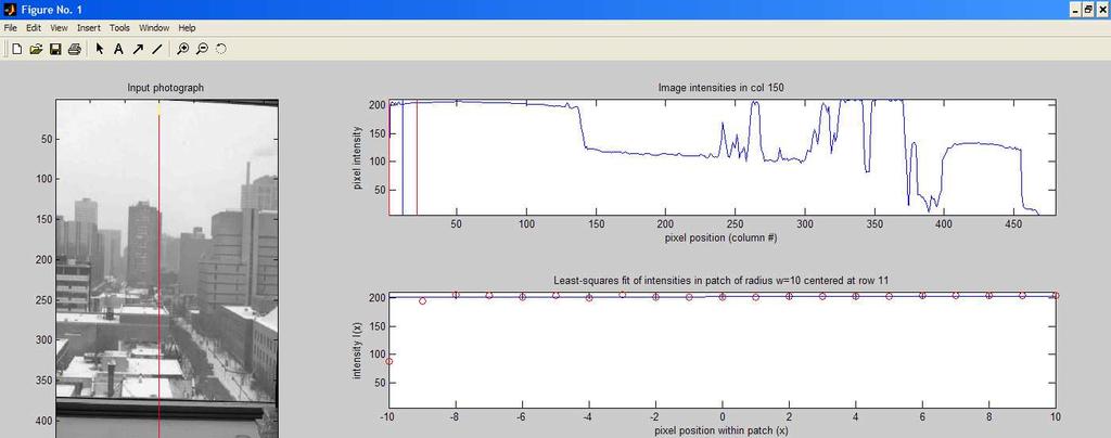
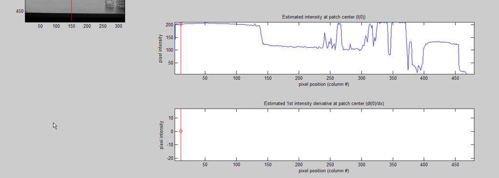
6 Estimating Intensities & their Derivatives Don t go, or you ll miss out!

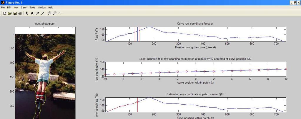
7 Representing & Analysing2D Curves, why? Useful representation for: Object boundaries Isophoteregions (groups of pixels with the same intensity)

8 Representing & Analysing2D Curves, how? Math is our friend: Provides an unambiguous representation Enables computation of useful properties

9 2D Image Curves: Definition A parametric 2D curve is a continuous mapping γ: (a,b) -> R 2 where t -> (x(t), y(t))

10 2D Image Curves: Definition Example: a boundary curve t = pixel # along the boundary x(t) = x coordinate of the t th pixel y(t) = y coordinate of the t th pixel

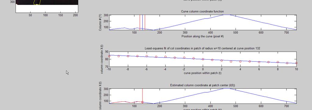
11 2D Image Curves: Definition To fully describe a curve we need the two functions x(t)and y(t), called the Coordinate Functions.

12 2D Image Curves: Definition A closed2d curve is a continuous mapping γ: (a,b) -> R 2 where t -> (x(t), y(t)) such that (x(a), y(a)) = (x(b), y(b)).

13 Smooth 2D Curves A curve is smooth when...

14 Smooth 2D Curves A curve is smooth when all the derivatives of the Coordinate Functions exist

15 Derivatives of the Coordinate Functions The 1 st and 2 nd derivatives of x(t), y(t) are extremely informativeabout the shape of a curve.

16 Topic 4.2: Local analysis of 2D curve patches Representing 2D image curves Estimating differential properties of 2D curves Tangent & normal vectors The arc-length parameterization of a 2D curve The curvature of a 2D curve

17 The Tangent Vector Notation: γ(t) = (x(t), y(t)) γ(t) maps a number (t) to a 2D point (x(t), y(t)). This type of function is called a vector-valued function.

18 The Tangent Vector γ(t) Suppose we know γ(0). γ(0) = (x(0), y(0)) How can we approximate γ(t)?

19 The Tangent Vector γ(t) Suppose we know γ(0). γ(0) = (x(0), y(0)) How can we approximate γ(t)? hint?

20 The Tangent Vector γ(t) Suppose we know γ(0). γ(0) = (x(0), y(0)) How can we approximate γ(t)? Using the derivative (tangent)!

21 The Tangent Vector γ(t) Suppose we know γ(0). γ(0) = (x(0), y(0)) How can we approximate γ(t)? Using the derivative (tangent)!

22 The Tangent Vector γ(t) Prediction of γ(t) γ(0) = (x(0), y(0)) Good! But not great. Can we do any better? If so, how?

23 The Tangent Vector γ(t) Prediction of γ(t) γ(0) = (x(0), y(0)) Good! But not great. Add more information about the curve, like the 2 nd, 3 rd, or the n th derivative! Familiar?

24 The Tangent Vector γ(t) Prediction of γ(t) γ(0) = (x(0), y(0)) Good! But not great. Add more information about the curve, like the 2 nd, 3 rd, or the n th derivative! This is a Taylor-Series approximation

25 The Tangent Vector γ(t) Formally: the 1 st order Taylor-Series approximation to γ(t) near γ(0) is:, so γ(0)= (x(0), y(0))

26 The Tangent Vector γ(t) γ(0) Definition. The tangent vector at γ(t) is equal to the first derivative of the function, at that point. In this case: 1 st order Taylor- Series approximation of γ(t) at t=0

27 The Tangent Vector γ(t) γ(0) In general, the derivative of a vector valued function is the derivative of the n coordinate functions, so if The derivative of f at (t) is:

28 Effect of Curve Parameter on the Tangent We can parameterize a curve γin (infinitely) many different ways, for instance: 1. Make t the number of pixels between γ(0) and γ(t) 2. Make t the actual length of the curve between γ(0) and γ(t), in meters (or inches, or light-years).

29 Effect of Curve Parameter on the Tangent We can parameterize a curve γin (infinitely) many different ways, for instance: 1. Make t the number of pixels between γ(0) and γ(t) 2. Make t the actual length of the curve between γ(0) and γ(t), in meters (or inches, or light-years). But the key property is that the direction of the tangent remains unchanged, regardless of the scale of the parameter.

30 Effect of Curve Parameter on the Tangent The direction of the tangent remains unchanged, regardless of the scale of the parameter. Really? Can we prove it?

31 Effect of Curve Parameter on the Tangent Proof: Let s parameterize the curve γ in two ways: 1. Take t = the number of pixels between γ(0) and γ(t) 2. Take s = f(t) as the parameter, wheref(t) is simply any differentiable function.

32 Effect of Curve Parameter on the Tangent Proof: Let s parameterize the curve γ in two ways: 1. Take t = the number of pixels between γ(0) and γ(t) 2. Take s = f(t) as the parameter, wheref(t) is simply any differentiable function. In 1, we know the derivative of γ is simply

33 Effect of Curve Parameter on the Tangent Proof: Let s parameterize the curve γ in two ways: 1. Take t = the number of pixels between γ(0) and γ(t) 2. Take s = f(t) as the parameter, wheref(t) is simply any differentiable function. In 1, we know the derivative of γ is simply In 2, the chain rule tells us that if s=f(t) and γ(s) then: which correspond to

34 Effect of Curve Parameter on the Tangent Proof: Let s parameterize the curve γ in two ways: 1. Take t = the number of pixels between γ(0) and γ(t) 2. Take s = f(t) as the parameter, wheref(t) is simply any differentiable function. In 1, we know the derivative of γis simply In 2, the chain rule tells us that if s=f(t) and γ(s) then:

35 The Unit Tangent Vector Definition. The Unit Tangent is: The unit tangent vector does not depend on the choice of the parameter t

36 The Arc-Length of a Curve How can we approximate the length of a curve?

37 The Arc-Length of a Curve

38 The Arc-Length of a Curve Take small enough steps (of size t) and add!

39 The Arc-Length of a Curve Take small enough steps (of size t) and add!

40 The Arc-Length of a Curve

41 The Arc-Length of a Curve This is called a piece-wise-linear length approximation. And what if we make the steps smaller and smaller? t-> 0

42 The Arc-Length of a Curve Then we get the following definition! The arc-length s(t) of the curve γ(t) is given by:

43 The Arc-Length of a Curve For example, lets think about the circle What do we expect

44 The Arc-Length of a Curve For example, lets think about the circle Proportional to the radius and the number of pixels in the circle

45 The Arc-Length of a Curve Example: The arc length of a circle with radius r, whose curve equation can be written as: γ(t) = r ( cos(t), sin(t) ) then so unit vectors

46 The Arc-Length of a Curve Example: The arc length of a circle with radius r, whose curve equation can be written as: γ(t) = r ( cos(t), sin(t) ) Now, substituting on the definition, we get:

47 The Arc-Length of a Curve Example: The arc length of a circle with radius r, whose curve equation can be written as: γ(t) = r ( cos(t), sin(t) ) Now, substituting on the definition, we get: Proportional to the radius yes! Proportional to the number of pixels in the circle yes!

48 The Arc-Length of a Curve Now, can we parameterize the function γ(t) using the arc-length function itself?

49 The Arc-Length of a Curve Now, can we parameterize the function γ(t) using the arc-length function itself? Yes!

50 The Arc-Length of a Curve Now, can we parameterize the function γ(t) using the arc-length function itself? Yes! A parameterization γ(s) where the curve parameter is the arclength is (thoughtfully and originally) named the arc-length parameterization.

51 The Arc-Length of a Curve Now, can we parameterize the function γ(t) using the arc-length function itself? Yes! Lets use the circle again as an example. We know that the arclength of a circle is s(t) = rt, or for short s = rt. Which means that, so the arc-length parameterization is:

52 The Arc-Length of a Curve Arc-length parameterization of the circle. Using γ(s) = the following holds: γ(t) = (x(t), y(t)) t

53 The Arc-Length of a Curve Now, we know that the arc-length is We also know that an arc-length parameterization γ(s) is one where the curve parameter is the arc-length Knowing these two facts, a property we can derive is that γ(s) is an arc-length parameterization of a curve if and only if

54 The Arc-Length of a Curve γ(s) is an arc-length parameterization of a curve if and only if

55 The Arc-Length of a Curve γ(s) is an arc-length parameterization of a curve if and only if This is a very useful property of arc-length parameterized curves, because the tangent -estimated as the derivative of the curve-is always a unit-tangent!

56 The Unit Normal Vector Let s look at the normal vector now

57 The Unit Normal Vector Today we learnt that the unit tangent is How do we estimate the Unit Normal?

58 The Unit Normal Vector Today we learnt that the unit tangent is As the orthogonal vector to T(t). As the orthogonal vector to T(t). The (unit) normal vector N(t) is the counter-clockwise rotation of T(t) by 90 degrees.

59 The Unit Normal Vector Today we learnt that the unit tangent is As the orthogonal vector to T(t). As the orthogonal vector to T(t). The (unit) normal vector N(t) is the counter-clockwise rotation of T(t) by 90 degrees.

60 The Unit Normal Vector Aside: what are orthogonal vectors? Vectors aand bare orthogonal if and only if their dot product is zero. So if a= [a x, a y ], and b= [b x, b y ], then a and bare orthogonal if and only if: a x a y b x = a x b x + a y b y = 0 b y

61 The Moving Frame Putting the unit Tangent and the unit Normal together we get: The Moving Frame, defined as the pair of orthogonal vectors {T(t), N(t)}

62 The Moving Frame For example, the circle

63 The Moving Frame Noteworthy: 1. As we change the parameter t, the moving frame rotates 2. The fasterthe frame rotates, the more curved the curve is 3. The speed at which the moving frame is rotating can be estimated using a 1 st order Taylor-series near t=0.

64 Topic 4.2: Local analysis of 2D curve patches Representing 2D image curves Estimating differential properties of 2D curves Tangent & normal vectors The arc-length parameterization of a 2D curve The curvature of a 2D curve

65 Arc-Length Parameterization: T(s) & N(s) We know that: The unit tangent is: And that the unit normal is the 90-deg counter-clockwise rotation: Note that we use s as the parameter to denote arc-length parameterizations. And we arc-length parameterizations because the expressions are simpler (see last slide of this lecture for comparison).

66 Defining the Curvature at a Point Theorem. Definition of curvature. If s is the arc-length of a curve, then

67 Defining the Curvature at a Point The traditional way of writing the 1 st order Taylor approximation of the moving frame is: But if we use the curvature k(s), it becomes

68 Defining the Curvature at a Point The 1 st order Taylor-series approximation becomes:

69 Defining the Curvature at a Point The 1 st order Taylor-series approximation becomes:

70 Defining the Curvature at a Point The 1 st order Taylor-series approximation becomes:

71 Defining the Curvature at a Point The 1 st order Taylor-series approximation becomes:

72 Defining the Curvature at a Point The 1 st order Taylor-series approximation becomes:

73 Defining the Curvature at a Point The 1 st order Taylor-series approximation becomes:

74 Defining the Curvature at a Point The 1 st order Taylor-series approximation becomes:

75 Defining the Curvature at a Point The 1 st order Taylor-series approximation becomes:

76 Defining the Curvature at a Point The 1 st order Taylor-series approximation becomes: And the scaling constant is k(s)

77 Defining the Curvature at a Point The 1 st order Taylor-series approximation becomes: And the scaling constant is k(s) What is this constant saying?

78 Defining the Curvature at a Point The 1 st order Taylor-series approximation becomes: And the scaling constant is k(s) What is this constant saying? How much of the Normaldo we need to add to the Tangent T(0) to approximate the tangent at T(t).

79 Interpreting the Sign of the Curvature k(s)

80 Interpreting the Absolute Value of k(s) What is the intuition of the above equation then? The equation is saying, look we can approximate γ(s) (by approximating the Tangent and the Normal) using a circle that: passes through γ(0), is tangent to T(0),and passes through γ(s)

81 The Arc-Length Parameterization & k(s) Example: the curvature of a circle of radius r. Parametric equation: g(t) = r (cost, sin t). Arc-length parameterization First derivative Second derivative

82 The Circle of Curvature k(s)

83 k(t) for Non-Arc-Length Parameterizations