Multivariate Analysis Multivariate Calibration part 2

Transcription

1 Multivariate Analysis Multivariate Calibration part 2 Prof. Dr. Anselmo E de Oliveira anselmo.quimica.ufg.br anselmo.disciplinas@gmail.com

2 Linear Latent Variables An essential concept in multivariate data analysis is the mathematical combination of several variables into a new variable that has a certain desired property. In chemometrics such a new variable is often called a latent variable Linear Latent Variable u = b 1 x 1 + b 2 x b m x m u scores, value of linear latent variable b j loadings, coefficients describing the influence of variables on the score x j variables, features.

3 Calibration Linear models y = b 0 + b 1 x 1 + b 2 x b j x j + + b m x m + e b 0 is called the intercept b 1 to b m the regression coefficients m the number of variables e the residual (error term) Often mean-centered data are used and then b 0 becomes zero This model corresponds to a linear latent variable.

4 Calibration The parameters of a model are estimated from a calibration set (training set) containing the values of the x-variables and y for n samples (objects) The resulting model is evaluated with a test set (with know values for x and y) Because modeling and prediction of the y-data is a defined aim of data analysis, this type of data treatment is called supervised learning.

5 Calibration All regression methods aim at the minimization of residuals, for instance minimization of the sum of the squared residuals It is essential to focus on minimal prediction errors for new cases the test set but no (only) for the calibration set from which the model has been created It is realatively ease to create a model especially with many variables and eventually nonlinear features that very well fits the calibration data; however, it may be useless for new cases. This effect of overfitting is a crucial topic in model creation.

6 Calibration Regression can be performed directly with the values of the variables (ordinary least-squares regression, OLS) but in the most powerful methods, such as principal component regression (PCR) and partial leastsquares regression (PLS), it is done via a small set of intermediate linear latent variables (the components). This approach has important advantages: Data with highly correlating x-variables can be used Data sets with more variables than samples can be used The complexity of the model can be controlled by the number of components and thus overfitting can be avoided and maximum prediction performance for test set data can be approached.

7 Calibration Depending on the type of data, different methods are available Number of x-variables Number of y-variables Name Methods 1 1 Simple Simple OLS, robust regression Many 1 Multiple PLS, PCR, multiple OLS, robust regression, Ridge regression, Lasso regression Many Many Multivariate PLS2, Canonical Correlation Analysis (CCA)

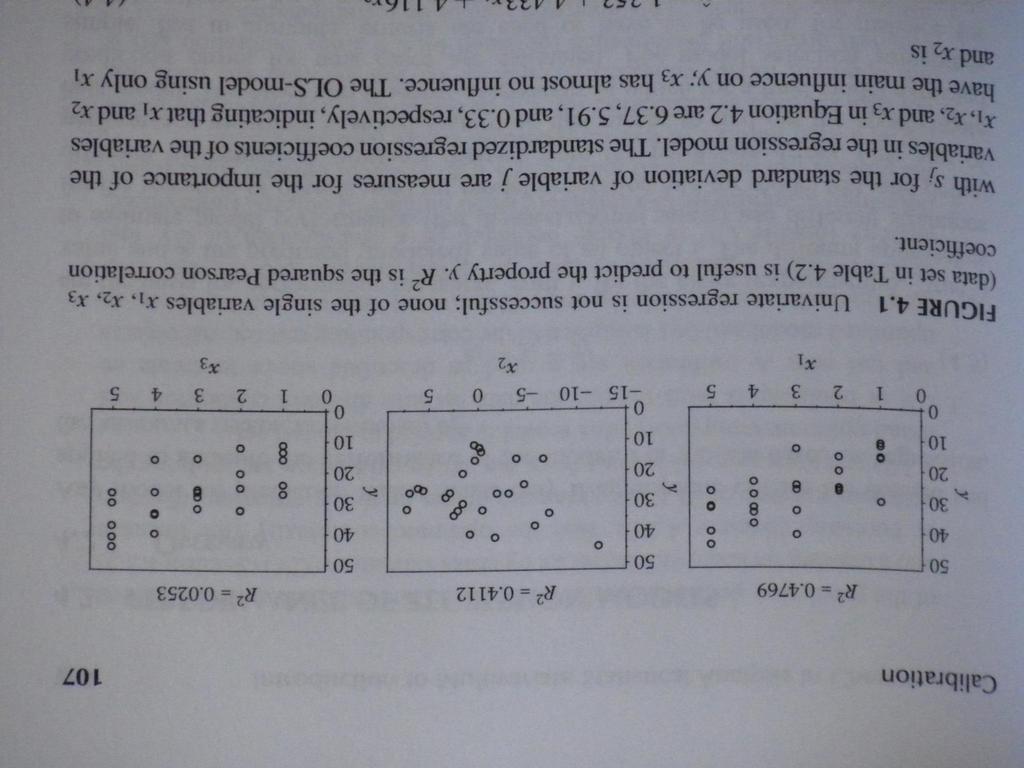
8 Calibration y = x x x 3

9 Calibration

10 Calibration OLS-model using only x 1 and x 2 y = x x 2

11 Performance of Regression Models Any model for prediction makes sense only if appropriate criteria are defined and applied to measure the performance of the model For models based on regression, the residuals (prediction errors) e i e i = y i y i are the basis for performance measures, with y i for the given (experimental, true ) value and y i the predicted (modeled) value of an object i An often-used performance measure estimates the standard deviation of the prediction errors (standard error of prediction, SEP).

12 Performance of Regression Models Using the same objects for calibration and test should be strictly avoided Depending on the size of the data set (the number of objects available) and on the effort of work different strategies are possible The following levels are ordered by typical applications to data with decreasing size and also by decreasing reliability of the results.

13 Performance of Regression Models 1. If data from many objects are available, a split into three sets is best: i. Training set (ca. 50% of the objects) for creating models ii. Validation set (ca. 25% of the objects) for optimizing the model to obtain good prediction performance iii. Test set (prediction set, approximately 25%) for testing the final model to obtain a realistic estimation of the prediction performance for new cases iv. The three sets are treated separately v. Applications in chemistry rarely allow this strategy because of a too small number of objects available.

14 Performance of Regression Models 2. The data is split into a calibration set used for model creation and optimization and a test set (prediction set) to obtain a realistic estimation of the prediction perfomance for new cases i. The calibration set is divided into a training set and a ii. validation set by cross validation (CV) or bootstrap First the optimum complexity (for instance optimum number of PLS components) of the model is estimated and then a model is built from the whole calibration set applying the found optimum complexity; this model is applied to the test set.

15 Performance of Regression Models 3. CV or bootstrap is used to split the data set into different calibration sets and test sets i. A calibration set is used as described (2) to create an optimized model and this is applied to the corresponding ii. iii. test set All objects are principally used in training set, validation set, and test set; however, an object is never simultaneously used for model creations and for test This strategy (double CV or double bootstrap or a combination of CV and bootstrap) is applicable to a relatively small number of objects; furthermore, the process can be repeated many times with different random splits resulting in a high number of test-setpredicted values.

16 Performance of Regression Models Mostly the split of the objects intro training, validation, and test sets is performed by simple random sampling More sophisticated procedures related to experimental design and theory of sampling are available Kennard-Stone algorithm it claims to set up a calibration set that is representative for the population, to cover the x-space as uniformly as possible, and to give more weight to objects outside the center This aim is reached by selecting objects with maximum distances (for instance Euclidean distances) in the x-space.

17 Performance of Regression Models The methods CV and bootstrap are called resampling strategies Small data sets They are applied to obtain a reasonable high number of predictions The larger the date set and the more reliable the data are, the better the prediction performance can be estimated size of the data friendliness of data uncertainty of performance measure = constant.

18 Overfitting and Underfitting The more complex (the larger ) a model is, the better is it capable of fit given data (the calibration set) The prediction error for the calibration set in general decreases with increasing complexity of the model An appropriate highly complicated model can fit almost any data with almost zero deviations (residuals) between experimental (true) y and modeled (predicted) y Such model are not necessarily useful for new cases, because they are probably overfitted.

19 Overfitting and Underfitting Fonte da Imagen: Dr. Frank Dieterle

20 Overfitting and Underfitting Fonte da Imagen: holehouse.org

21 Overfitting and Underfitting Prediction error for new cases are high for small models (underfitting, low complexity, too simple models) but also for overfitted models Determination of the optimum complexity of a model is an important but not always na easy task, because the minumum of measures for the prediction error for test sets is often not well marked In chemometrics, the complexity is typically controled by the number of PLS or PCA components (latent variables), and the optimum complexity is estimated by CV CV or bootstrap allows an estimation of the prediction error for each object of the calibration set at each considered model complexity.

22 Performance Criteria The basis of all perfomence criteria are prediction errors (residuals) y i y i The classical standard deviation of prediction errors is widely used as a measure of the spread of the error distribution, and is called standard error of prediction (SEP) defined by with SEP = 1 z 1 z i=1 z y i y i bias 2 bias = 1 z where y i are the given (experimental, true ) values y i are the predicted (modeled) values z is the number of predictions. i=1 y i y i

23 Performance Criteria The bias is the arithmetic mean of the prediction errors and should be near zero A systematic error (a nonzero bias) may appear if, for instance, a calibration model is applied to data that have been produced by another instrument In the case of a normal distribution, about 95% of the prediction errors are within the tolerance interval 2 SEP The measure SEP and the tolerance interval are given in the units of y.

24 Performance Criteria Standard error of calibration (SEC) is similar to SEP applied to predictions of the calibration set The mean squared error (MSE) is the arithmetic mean of the squared errors z MSE = 1 y z i y 2 i i=1 MSEC refers to results from a calibration set, MSECV to results obtained in CV, and MSEP to results from a prediction/test set MSE minus the squated bias gives the squared SEP SEP 2 = MSE bias 2.

25 Performance Criteria The root mean squared error (RMSE) is the square root of MSE, and can again be given for calibration (RMSEC), CV (RMSECV) or for prediction/test (RMSEP) RMSE = 1 z z i=1 y i y i 2 MSE is preferably used during the development and optimization of models but is less useful for practical applications because it has not the units of the predicted property A similar widely used measure is predicted residual error sum of squares (PRESS), the sum of the squared errors z PRESS = y i y 2 i=1 i = z MSE.

26 Performance Criteria Correlation measures between experimental y and predicted y are frequently used to characterize the model performance Mostly used is the squared Pearson correlation coefficient.

27 Criteria for Models with Different Numbers of Variables The model should not contain a too smal number of variables because this leads to poor prediction performance. On the other hand, it should also not contain a too large number of variables because this results in overfitting and thus again poor prediction performance 2 The adjusted R-square, R adj 2 R adj or R = 1 n 1 n m 1 1 R2 where n is the number of objects m is the number of regressor variables (including the intercept) R 2 is called coefficient of determination, expressing the proportion of variance that is explained by the model.

28 Criteria for Models with Different Numbers of Variables 2 Another, equivalent representation for R adj RSS n m 1 2 R adj = 1 TSS n 1 with residual sum of squares (RSS) for the sum of the squared residuals n RSS = y i y i 2 i=1 and the total sum of squares (TSS) for the sum of the squared differences to the mean y of y, n TSS = y i y 2 i i=1. is

29 Cross Validation (CV) It is the most used resampling strategy to obtain a reasonable large number of predictions It is also often applied to optimize the complexity of a model The optimum number of PLS or PCA components To split the data into calibration sets and test sets.

30 Cross Validation (CV) The procedure of CV applied to model optimization The available set with n object is randomly split into s segments (parts) of approximately equal size The number of segments can be 2 to n, often values between 4 to 10 are used One segment is left out as a validation set The other s 1 sets are used as a training set to create models which have increasing complexity (for instance, 1,2,3,, a max PLS components) The models are separately applied to the objects of the validation set resulting in predicted values connected to different model complexities This procedure is repeated so that each segment is a validation set once The result is a matrix with n rows and a max colums containing predicted values y CV (predicted by CV) for all objects and all considered model complexities From this matrix and the known y-values, a residual matrix is computed An error measure (for instance MSECV) is calculated from the residuals, and the lowest MSECV or a similar criterion indicates the optimum model complexity.

31 Cross Validation (CV) K. Baumann, TrAC 2003, 22(6), 395

32 Cross Validation (CV) A single CV gives n predictions For many data sets in chemistry n is too small for a visualization of the error distribution The perfomance measure depends on the split of the objects into segmentes Is therefore recommended to repeat the CV with different random splits into segments (repeated CV), and to summarize the results.

33 Cross Validation (CV) If the number of segments is equal to the number of objects (each segment contains only one object), the method is called leave-one-out CV or full CV Randomization of the sequence of objects is senseless, therefore only one CV run is necessary resulting in n predictions The number of created models is n which may be timeconsuming for large data sets Depending on the data, full CV may give too optimistic results, especially if pairwise similar objects are in the data set, for instance from duplicate measurements Full CV is easier to apply than repeated CV or bootstrap In many cases, full CV gives a reasonable first estimate of the model performance.

34 Bootstrap As a verb, bootstrap has survived into the computer age, being the origin of the phrase "booting a computer." "Boot" is a shortened form of the word "bootstrap," and refers to the initial commands necessary to load the rest of the computer's operating system. Thus, the system is "booted," or "pulled up by its own bootstraps"

35 Bootstrap Within multivariate analysis, bootstrap is a resampling method that can be used as na alternative to CV, for instance, to estimate the prediction performance of a model or to estimate the optimum complexity In general, bootstrap can be used to estimate the distribution of model parameters Basic ideas of bootstraping are resampling with replacement, and to use calibration sets with the same number of objects, n, as objects are in the available data set A calibration set is obtained by selecting randomly objects and copying (not moving) them into the calibration set Toolbox.

36 Ordinary Least-Squares Regression

37 Simple OLS y = b 0 + bx + e b and b 0 are the regression parameters (regression coefficients) b 0 is the intercept and b is the slope Since the data will in general not follow a perfect linear relation, the vector e contains the residuals (errors) e 1, e 2,, e n.

38 Simple OLS The predicted (modeled) property y i for sample i and the prediction error e i are calculated by y i = b 0 + bx i e i = y i y i The Ordinary Least-Squares (OLS) approach minimizes the sum of the squared residuals e 2 i to estimate the model parameters b and b 0 n i=1 x i x y i y b = n x i x 2 i=1 b 0 = y bx For mean-centered data (x = 0, y = 0), b 0 = 0 and b = n i=1 n i=1 x i y i x i 2 = xt y x T x.

39 Simple OLS The described model best fits the given (calibration) data, but is not necessarily optimal for predictions The least-squares approach can become very unreliable if outliers are present in the data Assumption for obtaining reliable estimates Errors are only in y but not in x Residuals are uncorrelated and normally distributed with mean 0 and constant variance σ 2 (homoscedasticity).

40 Simple OLS The following scatterplots are plots of x i (measurement) vs. i (observation number) with the sample mean marked with a red horizontal line. The measurement is plotted on the vertical axis; the observation number is plotted on the horizontal axis Unbiased The average of the observations in every thin vertical strip is the same all the way across the scatterplot. Biased The average of the observations changes, depending on which thin vertical strip you pick. Homoscedastic The variation (σ) of the observations is the same in every thin vertical strip all the way across the scatterplot. Heteroscedastic The variation (σ) of the observations in a thin vertical strip changes, depending on which vertical strip you pick. (a) unbiased and homoscedastic (b) unbiased and heteroscedastic (c) biased and homoscedastic (d) biased and heteroscedastic (e) unbiased and heteroscedastic (f) biased and homoscedastic

41 Simple OLS Besides estimating the regression coefficients, it is also of interest to estimate the variation of the measurements around the fitted regression line. This means that the residual variance σ 2 has to be estimated s e 2 = 1 n 2 n i=1 y i y i 2 = 1 n 2 The denominator n 2 is used here because two parameters are necessary for a fitted straight line, and this makes s e 2 an unbiased estimator for σ 2 Confidence intervals for intercept and slope b 0 ± t n 2;p s b 0 b ± t n 2;p s b Standard deviations of b 0 and b n 2 i=1 x s b 0 = s i e n n x i x 2 s b = n x i x 2 i=1 t n 2;p is the p-quantile of the t-distribution witn n 2 degress of freedom, with for instance p = for a 95% confidence interval. i=1 s e n i=1 e i 2

42 Simple OLS Confidence interval for the residual variance σ 2 n 2 s2 e 2 < σ 2 < n 2 s e 2 2 χ n 2;1 p χ n 2;p 2 2 where χ n 2;1 p and χ n 2;p are the appropriate quantiles of the chisquare distribution (ref 1, table) with n 2 degrees of freedom (e.g., p = for a 95% confidence interval) Null hypothesis H 0 : b 0 = 0 T b0 = b 0 s b 0 H 0 is rejected at the significance level of if T b0 > t n 2;1 α 2 The test for b = 0 is equivalent T b = b s b.

43 Simple OLS Often it is of interest to obtain a confidence interval for the prediction at a new x value 1 y ± s e 2F 2,n 2;p n + x x 2 n x x 2 i=1 with F 2,n 2;p the p-quantile of the F-distribution with 2 and n 2 degrees of freedrom Best predictions are possible in the mid part of the range of x where most information is available.

44 Simple OLS Using the open source software (An Introduction to R) > x=c(1.5,2,2.5,2.9,3.4,3.7,4,4.2,4.6,5,5.5,5.7,6.6) > y=c(3.5,6.1,5.6,7.1,6.2,7.2,8.9,9.1,8.5,9.4,9.5,11.3,11.1) > res<-lm(y~x) # linear model for y on x. The symbol ~ # allows to construct a formula for the relation > plot(x,y) > abline(res)

45 Simple OLS > summary(res) Call: lm(formula = y ~ x) b 0 and b Residuals: Min 1Q Median 3Q Max s b 0 and s b T b 0 and T b Coefficients: Estimate Std. Error t value Pr(> t ) (Intercept) ** x e-06 *** --- Signif. codes: 0 *** ** 0.01 * Residual standard error: on 11 degrees of freedom Multiple R-squared: , Adjusted R-squared: F-statistic: on 1 and 11 DF, p-value: 1.049e-06 in the case of univariate x and y is the same as the squared Pearson correlation coefficient, and it is a measure of model fit first quartile is the value in which 25% of the numbers are below it s e tests wheter all parameters are zero, against the alternative that at least one regression parameter is different from zero. Since the p-value ~0, at least one of intercept or slope contributes to the regression model since p-values are much smaller than a reasonable significance level, e,g, α = 0.05, both intercept and slope are important in our regression model

46 Muliple OLS y 1 = b 0 + b 1 x 11 + b 2 x b m x 1m + e 1 y 2 = b 0 + b 1 x 21 + b 2 x b m x 2m + e 2 y n = b 0 + b 1 x n1 + b 2 x n2 + + b m x nm + e n or y = Xb + e Multiple Linear Regression Model X of size n m + 1 which includes in its first column n values of 1 The residuals are calculated by e = y y The regression coefficients b = b 0, b 1,, b T m result from the OLS estimation minimizing the sum of squared residuals e T e b = X T X 1 X T y.

47 Muliple OLS Confidence Intervals and Statistical Tests The following assumptions must be fulfilled Erros e are independent n-dimensional normally distributed With mean vector 0 And covariance matrix σ 2 I n An unbiased estimator for the residual variance σ 2 is n s e 2 = 1 n m 1 y i y i 2 = 1 n m 1 y Xb T y Xb i=1 The null hypothesis b j = 0 against the alternative b j 0 can be tested with the test statistic b j z j = s e d j where d j is the jth diagonal element of X T X 1 The distribution of z j is t n m 1, and thus a large absolute value of z j will lead to a rejection of the null hypothesis F-test can also be constructed to test the null hypothesis b 0 = b 1 = = b m = 0 against the alternative b j 0 for any j = 0,1,, m.

48 Multiple OLS Using the open source software R > T=c(80,93,100,82,90,99,81,96,94,93,97,95,100,85,86,87) > V=c(8,9,10,12,11,8,8,10,12,11,13,11,8,12,9,12) > y=c(2256,2340,2426,2293,2330,2368,2250,2409,2364,2379,2440,2364,2404,2317,2309,2328) > res<-lm(y~t+v) # linear model for y on T and V. The symbol ~ # allows to construct a formula for the relation > summary(res) Call: lm(formula = y ~ T + V) Residuals: Min 1Q Median 3Q Max Coefficients: Estimate Std. Error t value Pr(> t ) (Intercept) e-12 *** T e-08 *** V ** --- Signif. codes: 0 *** ** 0.01 * Residual standard error: on 13 degrees of freedom Multiple R-squared: 0.927, Adjusted R-squared: F-statistic: 82.5 on 2 and 13 DF, p-value: 4.1e-08

49 Hat Matrix The hat-matrix H combines the observed and predicted y-values y = Hy and so it puts the hat on y. The hat-matrix is defined as H = X X T X 1 X T the diagonal elements h ii of the n n matrix H reflet the influence of each value y i on its own prediction y i.

50 Multivariate OLS Multivariate Linear Regression relates several y-variables with several x-variables Y = XB + E In terms of a single y-variable OLS estimator for b j resulting in and y j = Xb j + e j b j = X X T X 1 X T y j B = X X T X 1 X T Y Y = XB Matrix B consists of q loading vectors, each defining a direction in the x-space for a linear latent variable which has maximum Pearson s correlation coefficient between y j and y j for j = 1,, q The regression coefficients for all y-variables can be computed at once, however, only for noncollinear x-variables and if m < n m x-variables, n observations, and q y-variables Alternative methods are PLS2 and CCA.

51 Variable Selection Feature selection For multiple regression all available variables x 1, x 2,, x m were used to build a linear model for the prediction of the y-variable Useful as long as the number m of regressor variables is small, say not more than 10 OLS regression is no longer computable if the Regressor variables are highly correlated Number of objects is lower than the number of variables PCR and PLS can handle such data.

52 Variable Selection Arguments against the use of all available regressor variables Use of all variable will produce a better fit of the model for the training data The residuals become smaller and thus the R 2 measure increases We are usually not interested in maximizing the fit for the training data but in maximizing the prediction performance for the test data Reduction of the regressor variables can avoid the effects of overfitting A regression model with a high number of variables is pratically impossible to interpret.

53 Variable Selection Univariate and Bivariate Selection Methods Criteria for the elimination of regressor variables A considerable percentage of the variable values is missing of below a small threshold All or nearly all variable values are equal The variable includes many and severe outliers Compute the correlation between pairs of regressor variables. If the correlation is high (positive or negative), exclude that variable having the larger sum of (absolute) correlation coefficients to all remaining regressor variables.

54 Variable Selection Criteria for the identification of potentially useful regressor variables High variance of the variable High (absolute) correlation coefficient with the yvariable.

55 Variable Selection Stepwise Selectrion Methods Adds or drops one variable at a time Forward selection Start with the empty model (or with preselected variables) and add that variable to the model that optimizes a criterion Continue to add variables until a stopping rule becomes active Backward elimination Start with the full model... Both directions.

56 Variable Selection An often-used version of stepwise variable selection works as follows Select the variable with highest absolute correlation coefficient with the y-variable; the number of selected variables is m 0 = 1 Add each of the remaining x-variables separately to the selected variable; the number of variables in each subset is m 1 = 2 Calculate F F = RSS 0 RSS 1 m 1 m 0 RSS 1 n m 1 1 with RSS being the sum of the squared residuals y i y i 2 n i=1 Consider the added variables which gives the highest F, and if the decrease of RSS is significant, take this variable as the second selected one Significance: F > F m1 m 0,n m 1 1;0.95 Forward selection of variables would continue in the same way until no significant change occurs Disadvantage: a selected variable cannot be removed later on» Usually the better strategy is to continue with a backwad step» Another forward step is done, followed by another backward step, and so on, until no significant change of RSS occurs or a defined maximum number of variables is reached.

57 Variable Selection Best-Subset/All-Subsets Regression Allows excluding complete branches in the tree of all possible subsets, and thus finding the best subset for data sets with up to about variables Leaps and Bounds algorithm or regression-tree methods Model selection Adjusted R 2 Akaike s Information Criterion (AIC) AIC = nlog RSS + 2m n Bayes Information Criterion (BIC) Mallow s Cp.

58 Variable Selection x 1 + x 2 + x 3 x 1 + x 2 AIC = 10 x 1 + x 3 x 2 + x 3 AIC = 20 x 1 AIC > 8 x 2 AIC > 18 x 3 AIC > 18 Since we want to select the model which gives the smallest value of the AIC, the complete branch with x 2 + x 3 can be ignored, bacause any submodel in this branch is worse (AIC > 18) than the model x 1 + x 2 with AIC = 10

59 Variable Selection Variable Selection Based on PCA or PLS Models These methods form new latent variables by using linear combinations of the regressor variables b 1 x 1 + b 2 x b m x m The coefficients/loadings reflect the importance of an x-variable for the new latent variable The absolute size of the coefficients can be used as a criterion for variable selection.

60 Variable Selection Genetic Algorithms (GAs) Natural Computation Method

61 Variable Selection Gene Population Delete chromosomes with poor fitness (selection) Create new chromosomes from pairs of good chromosomes (crossover) Change a few genes randomly (mutation) New (better) population

62 Variable Selection Crossover two chromosomes are cut at a random position and the parts are connected in a crossover scheme resulting in two new chromosomes

63 Variable Selection Cluster Analysis of Variables Cluster analysis tries to identify homogenous groups in the data If it is applied to the correlation matix of the regressor variables, one may obtain groups of variables that are strongly related, while variables in different groups will have a weak correlation.