An introduction to SPSS

Size: px

Start display at page:

Download "An introduction to SPSS"

Bernard Carter
6 years ago
Views:

1 An introduction to SPSS To open the SPSS software using U of Iowa Virtual Desktop... Go to and choose SPSS 24. Contents NOTE: Save data files in a drive that is accessible from virtual desktop. This is probably your H : drive through the university. 1 Example SPSS Data Set from UCLA 2 2 Uploading data to SPSS SPSS User Windows Data View Variable View Output Viewer Simple Plots and Correlation in SPSS Bar Chart Scatterplots Correlation Variable manipulation Standardizing Variables Transforming or Combining Variables Dichotomizing a continuous variable Logistic Regression 10 6 Two-way tables (categorical variables) 11 7 Split-plot with whole plot as CRD (Type I, assumes sphericity) Using General Linear Model with Repeated option Format of data Modeling the data SPSS output for tests Profile plots (means) SAS output for same example Comment on Residuals Using Mixed Models option Format of data Modeling the data SPSS output for tests

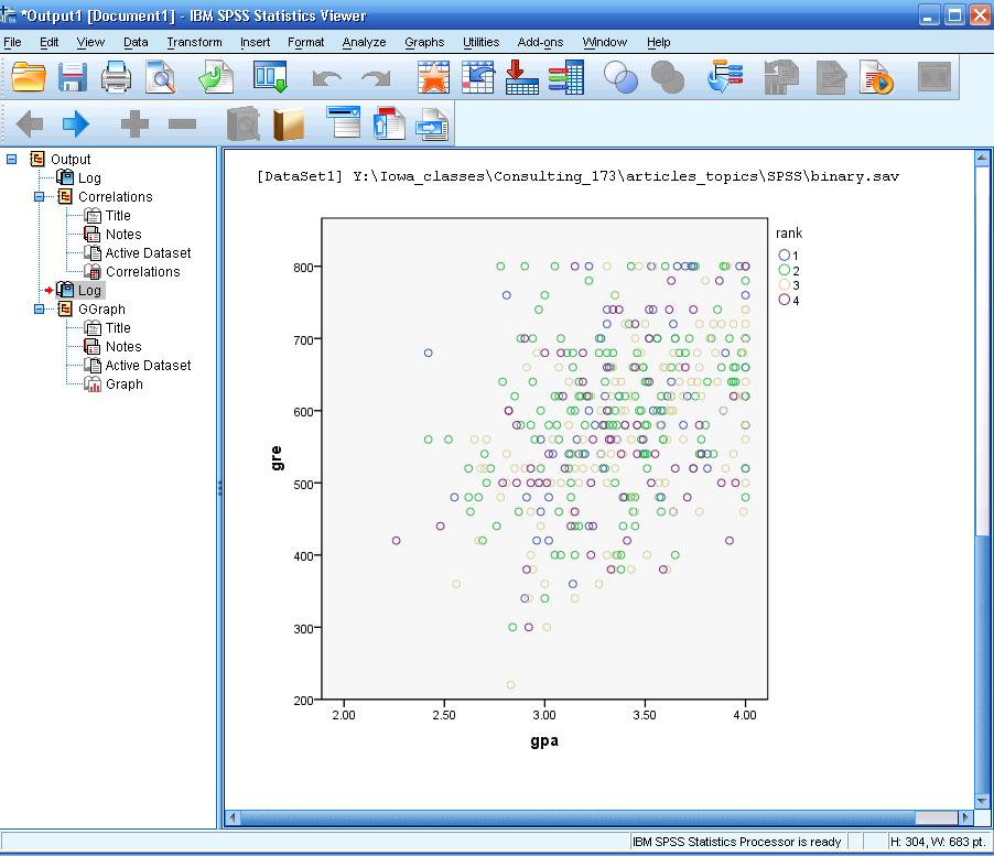
2 1 Example SPSS Data Set from UCLA UCLA Academic Technology Services has some nice statistical software examples available on-line, and we will utilize one of their SPSS data sets for this introduction. The data file is called binary.sav, and it is available at the URL below, and also at our class website in the datasets link. This data set contains variables related to admission to graduate school. Variables: admit -- Admission status to graduate school (0=no, 1=yes). gre -- Graduate Record Exam scores. Values range from 200 to 800. gpa -- Grade Point Average. rank -- Prestige of undergraduate school. Values are 1 through 4. Institutions with a rank of 1 have the highest prestige, while those with a rank of 4 have the lowest. 2 Uploading data to SPSS Open the binary.sav in SPSS using File Open Data SPSS User Windows Upon opening SPSS, you ll see the window called Data Editor. Within this window, you have two views of the data from which to choose. One looks like a spreadsheet of the actual data (Data View), and the other gives you information on the variables in the data set (Variable View). You can move back and forth between the windows by clicking on the respective tab at the bottom left of the window. After you import data or run any options, you will also see an Output Viewer window appear Data View Can be used in a manner similar to a spreadsheet. Allows user to enter Data. A new column can be entered (Highlight the column location, then Edit Insert Variable). A new row can be entered (Highlight the row location, Edit Insert Cases). You can use a formula to create a new variable, or transform a variable. 2

3 2.1.2 Variable View Allows user to input characteristics of variables (attributes, coding for missing values, the levels of class variables, etc.). Allows user to quickly view overall characteristics of the variables, like how many variables are in the data set, how many are categorical (nominal), or continuous (scale), etc. Many SPSS data sets arise from surveys and have 100 s of variables, which represent questions on the survey. It can take a long time to input this information, but is quite useful Output Viewer Contains the output generated by statistical procedures. Output location for graphics and plots. Can be saved separately from the.sav data file as a.spv file. Also serves as a log box. 3 Simple Plots and Correlation in SPSS NOTE: For the rest of the simple introduction (Sections 3-6), we will continue to use the binary.sav data set. ACTION REQUIRED: Change Variable Type Go to Variable View and make sure rank is set to ordinal. If not, change it to ordinal. 3.1 Bar Chart Graphs Chart Builder Bar Drag the Simple bar visual (1 st visual in top row) to the plotting area. Drag rank to the x-axis, click OK.! 3

4 3.2 Scatterplots Graphs Chart Builder You ll see the Chart Builder dialog box appear. Highlight Scatter/dot in the Gallery box. Drag the Grouped Scatter visual (2 nd visual in top row) to the plotting area. Drag gre to the x-axis and gpa to the y-axis. Drag rank to the set color box. Click OK (output appears in the Output Viewer box). 4

5 5

Highlight gre, then click the arrow to move it to the Variables box at the right.

6 3.3 Correlation Analyze Correlate Bivariate You ll see the Bivariate Correlations dialog box appear. Highlight gre, then click the arrow to move it to the Variables box at the right. Highlight gpa, then click the arrow to move it to the Variables box at the right. Click OK. The output will appear in the Output Viewer box, as below. 6

7 4 Variable manipulation 4.1 Standardizing Variables In SPSS, you can quickly standardize a variable and include the standardized z-scores as another column in the data set. Analyze Descriptive Statistics Descriptives... Highlight gre, then click the arrow to move it to the Variables box at the right. Highlight gpa, then click the arrow to move it to the Variables box at the right. Check the box: Save standardized values as variables. Click OK (the new variables will appear in the Data View). Run a correlation analysis on these two standardized variables and compare the results to the correlation analysis using the unstandardized. 7

.. Create a new variable called PreKnowledge which is the average

8 4.2 Transforming or Combining Variables Highlight an empty column in the Data View. Transform Compute Variable... Create a new variable called PreKnowledge which is the average of two standardized variables by inputting the formula: (Zgre+Zgpa)/2, then clicking OK. 8

4.3 Dichotomizing a continuous variable Transform Recode into Different Variables... You ll see the Recode into Different Variables dialog box appear. Highlight gre and put into the Variables box.

9 4.3 Dichotomizing a continuous variable Transform Recode into Different Variables... You ll see the Recode into Different Variables dialog box appear. Highlight gre and put into the Variables box. Provide a new name called codedgre in the Name box, and press Change. Click on Old and New Values. Under Old Value, select Range, LOWEST through value: 600 Under New Value, select Value: 0 Click Add Under Old Value, select Range, value through HIGHEST: 601 Under New Value, select Value: 1 Click Add, click Continue, click Change, click OK. The new variable will now appear in the Data View window. 9

10 5 Logistic Regression Analyze Generalized Linear Models Generalized Linear Models... On the Type of Model tab: choose binary logistic. On the Response tab: enter admit as dependent variable. Also... click Reference Category... and select First (lower value) in order to model the 1 s not 0 s. On the Predictors tab: enter rank as a Factor, enter gre, gpa as Covariates. On the Model tab: Include desired terms in the model. (For this example, highlight all and click main effects for simplicity. If you want to enter an interaction, highlight two variables at once, then choose Interaction.) Click OK. Generalized Linear Models Dependent Variable Probability Distribution Link Function admit a Binomial Logit Model Information a. The procedure models 1 as the response, treating 0 as the reference category. Case Processing Summary N Percent Included % Excluded 0 0.0% Total % Omnibus Test a Likelihood Ratio Chi-Square df Sig Dependent Variable: admit Model: (Intercept), rank, gre, gpa a. Compares the fitted model against the intercept-only model. Tests of Model Effects Type III Source Wald Chi- Square df Sig. (Intercept) rank gre gpa Dependent Variable: admit Model: (Intercept), rank, gre, gpa! 10

Parameter Estimates 95% Wald Confidence Interval Hypothesis Test Parameter B Std. Error Lower Upper Wald Chi- Square df Sig. (Intercept) -5.541 1.1381-7.772-3.311 23.709 1.000 [rank=1] 1.551.4178.

11 Parameter Estimates 95% Wald Confidence Interval Hypothesis Test Parameter B Std. Error Lower Upper Wald Chi- Square df Sig. (Intercept) [rank=1] [rank=2] [rank=3] [rank=4] 0 a gre gpa (Scale) 1 b Dependent Variable: admit Model: (Intercept), rank, gre, gpa a. Set to zero because this parameter is redundant. b. Fixed at the displayed value. - Output shows rank group 4 is the baseline (or reference) group. 6 Two-way tables (categorical variables)! Analyze Descriptive Statistics Crosstabs... Highlight admit and put into the Rows box. Highlight codedgre and put into the Columns box. Click on Cells... and under Percentages, choose Column Percentages, then Continue. Click on Statistics... and choose Chi-Squared, then Continue, then OK. 11

7 Split-plot with whole plot as CRD (Type I, assumes sphericity) This statistical model has a between-subject and within-subject factor (or factors). The example we use here was seen in STAT:5201.

There were two hamsters in each of the four between-subject treatment groups.

12 7 Split-plot with whole plot as CRD (Type I, assumes sphericity) This statistical model has a between-subject and within-subject factor (or factors). The example we use here was seen in STAT:5201. There were two factors (DayLength and Climate), each with two levels, that formed the four treatments in the between-subject effects. There was also one withinsubject factor (Tissue) with two levels. There were two hamsters in each of the four between-subject treatment groups. Thus, each hamster was nested in a particular DayLength/Climate combination and provided two observations in the analysis (one under each Tissue level). 7.1 Using General Linear Model with Repeated option Format of data One way to perform this analysis in SPSS is to approach it as a multivariate response. In that case, we need to format the data so that each row is associated with one hamster. Open the split plot hamsters.sav in SPSS using File Open Data Modeling the data Choose Analyze General Linear Models Repeated Measures... 12

Next, input the particular column names that coincide with the within-subject factor levels in the

13 Then give your within-subject factor a name (such as Tissue here) and state how many levels it has, then press Add and Define. Next, input the particular column names that coincide with the within-subject factor levels in the upper box, and define your model by inputting the between-subject factors in the appropriate box below (the default model includes all interactions between these factors). 13

If you dont want all of these results, you can select just specific main effects and interactions by using the Model button

14 Next, use the Options button to open the window below. This window will show you all the different interactions that will be tested as part of your analysis. If you dont want all of these results, you can select just specific main effects and interactions by using the Model button and the custom option in the main dialog window. Click Continue. Click the Save button and request to save the residuals and predicted values. This will save new columns in your present data set. Click Continue and then OK. 14

15 7.1.3 SPSS output for tests First, you ll get the within-subject tests. Tests of Within-Subjects Effects Measure: MEASURE_1 Source Tissue Tissue * DayLength Tissue * Climate Tissue * DayLength * Climate Error(Tissue) Sphericity Assumed Greenhouse-Geisser Huynh-Feldt Lower-bound Sphericity Assumed Greenhouse-Geisser Huynh-Feldt Lower-bound Sphericity Assumed Greenhouse-Geisser Huynh-Feldt Lower-bound Sphericity Assumed Greenhouse-Geisser Huynh-Feldt Lower-bound Sphericity Assumed Greenhouse-Geisser Huynh-Feldt Lower-bound Type III Sum of Squares df Mean Square F And then the between-subject tests farther down the in the output. Measure: MEASURE_1 Transformed Variable: Source Intercept DayLength Climate DayLength * Climate Error Tests of Between-Subjects Effects Average Type III Sum of Squares df Mean Square F Sig Page 1 15

16 7.1.4 Profile plots (means) You can also request some profile plots by clicking on the Plots... option and inputting horizontal axis variable (DayLength), separate lines variable(climate), and separate plots variable (Tissue). 16

17 Estimated Marginal Means of MEASURE_1 at Tissue = 1 Climate cold warm Estimated Marginal Means long DayLength short Estimated Marginal Means of MEASURE_1 at Tissue = 2 Climate cold warm Estimated Marginal Means Page long DayLength short 17

18 7.1.5 SAS output for same example From PROC MIXED, we see the tests for fixed effects are the same. Type 3 Tests of Fixed Effects Num Den Effect DF DF F Value Pr > F DayLength Climate DayLength*Climate Tissue DayLength*Tissue Climate*Tissue DayLen*Climat*Tissue From PROC GLM, we see all the sums of squares are equivalent, and we see that there are two distinct errors (for the whole-plot level and split-plot level) and this matches the SPSS output. Dependent Variable: NI The GLM Procedure Tests of Hypotheses for Mixed Model Analysis of Variance Source DF Type III SS Mean Square F Value Pr > F DayLength Climate DayLength*Climate Error Error: MS(Hamst(DayLen*Climat)) Source DF Type III SS Mean Square F Value Pr > F Tissue DayLength*Tissue Climate*Tissue DayLen*Climat*Tissue Hamst(DayLen*Climat) Error: MS(Error)

19 7.1.6 Comment on Residuals It looks like the residuals that you receive from SPSS are not the conditional residuals but rather the marginal residuals (what s leftover after accounting for the fixed effects). For checking the assumptions of the bottom-level noise (or σ 2 ), we want to consider the residuals after accounting for the random hamster effects, which are the conditional residuals. SPSS residuals and predicted values (only 8 predicted values in the plot): Normal Q-Q Plot Resids Sample Quantiles Preds Theoretical Quantiles SAS residuals and predicted values (more predicted values because they include the BLUPs): 19

20 The marginal residuals from SAS (this doesn t check our assumptions on ɛ ijk ): 20

7.2 Using Mixed Models option 7.2.1 Format of data For this modeling, we will have the data in

sav in SPSS using File Open Data... 7.2.2 Modeling the data Choose Analyze Mixed Models Linear.

21 7.2 Using Mixed Models option Format of data For this modeling, we will have the data in the same format as SAS, with one observation per row. Open the split plot hamsters format 2.sav in SPSS using File Open Data Modeling the data Choose Analyze Mixed Models Linear... and you will see the screen below to setup the subject factor. Once entered, click Continue. 21

22 Then choose your factors in the model (both fixed and random for now). Click on Fixed... to set-up fixed factors and press Continue. 22

Click on Random... to set-up the nested hamster effect. Choose the button Build nested terms and Include intercept. Highlight Hamster and click the down arrow.

23 Click on Random... to set-up the nested hamster effect. Choose the button Build nested terms and Include intercept. Highlight Hamster and click the down arrow. Click on (Within) and highlight DayLength and press the down arrow and then click on By* and highlight Climate and press the down arrow and then click Add then Continue. 23

24 Click the Save button and request to save the residuals and predicted values. This will save new columns in your present data set then click OK SPSS output for tests Type III Tests of Fixed Effects a Source Numerator df Denominator df F Sig. Intercept DayLength Climate Tissue DayLength * Climate DayLength * Tissue Climate * Tissue DayLength * Climate * Tissue a. Dependent Variable: NI Estimates of Covariance Parameters a Parameter Estimate Std. Error Residual Hamster(DayLength * Climate) a. Dependent Variable: NI. Variance Resid Pred And both the SPSS output above and the residuals match the SAS analysis. Page 1 24

Set up of the data is similar to the Randomized Block Design situation. A. Chang 1. 1) Setting up the data sheet

Set up of the data is similar to the Randomized Block Design situation. A. Chang 1. 1) Setting up the data sheet Repeated Measure Analysis (Univariate Mixed Effect Model Approach) (Treatment as the Fixed Effect and the Subject as the Random Effect) (This univariate approach can be used for randomized block design