The Pennsylvania State University. The Graduate School. College of Engineering THEORETICAL AND EXPERIMENTAL STUDIES OF AEROSOL PARTICLE DRAG

Transcription

1 The Pennsylvania State University The Graduate School College of Engineering THEORETICAL AND EXPERIMENTAL STUDIES OF AEROSOL PARTICLE DRAG MIXING IN TURBULENT FLOW A Thesis in Mechanical Engineering by Jason Wittenstein Submitted in Partial Fulfillment of the Requirements for the Degree of Master of Science August 2012

2 The thesis of Jason Wittenstein was reviewed and approved* by the following: Dan Haworth Professor of Mechanical Engineering Thesis Advisor Joseph J. Cor Thesis Co-Advisor Research Associate of the Applied Research Lab Tim Miller Senior Research Associate of the Applied Research Lab Karen Thole Professor or Mechanical Engineering Head of the Department of Mechanical Engineering *Signatures are on file in the Graduate School

3 iii ABSTRACT An experimental and theoretical study of the mixing of aerosol particles with highpressure gas under turbulent conditions to further the understanding of two-phase mixing is conducted. The Applied Research Laboratory has acquired laboratory characterizations of smallscale mixing, and these data are used as the basis for drag model development for a theoretical CFD study of two-phase mixing. This computational study focuses on gas-particle drag models, which are a critical part of accurately describing mixing phenomena in turbulent flow. The drag forces acting on the particles determine their entrainment relative to the gas medium, and determine how quickly they adjust to changes in the gas they are contained in. The availability of experimental data allows for testing of existing and refined drag models for their application to high-pressure, turbulent flow. Comparisons were made between three model formulations: single-phase, multi-phase, and Lagrangian analysis. In each case, results from a constant-drag-coefficient model were compared with those from a refined drag model, and model results were compared with experimental data. The refined drag models better predicted the spread angle of the aluminum particles, but overall under-predicted the recirculation radius compared to the constant-coefficient drag models.

4 iv TABLE OF CONTENTS LIST OF FIGURES... v LIST OF TABLES... viii ACKNOWLEDGMENTS... ix Chapter 1 Introduction... 1 Background... 1 Chapter 2 Data Extraction... 4 Vortex Chamber Description... 4 Velocity Calculations... 7 High Speed Video Analysis... 9 Spread Angle Particle Size Recirculation Radius Chapter 3 Description of Models Drag Model Eulerian Models Single-Phase Model Multi-phase Model Three Particle Size Model Lagrangian Model Transient Model Computational Grid Chapter 4 Test Analysis and Modeling Results Quantitative Data Comparison Test Test Test Test Chapter 5 Conclusion Future Work Appendix A Flow Rates Appendix B Velocity Calculations Fuel/Carrier Gas Appendix C Nitrogen Velocities Appendix D Spread Angle Screenshots Appendix E Particle Distribution Size Bibliography... 68

5 v LIST OF FIGURES Figure 1-1. Typical video image taken during test run... 2 Figure 1-2. Location and geometry of the test chamber... 2 Figure 2-1. Plastic ring injector flows Figure 2-2. Injector ring diagram Figure 2-3. Flow visualization chamber diagram Figure 2-4. Screenshot used to determine particle spread angle in Test Figure 2-5. Example of a measured recirculation radius Figure 3-1. Equation 5 vs. experiment (4) Figure 3-2. Fluent model versus experimental data Figure 3-3. Cheng model versus experimental data Figure 3-4. Morsi and Alexander model versus experimental data Figure 3-5. Steps involved in the SIMPLE algorithm (15) Figure 3-6. Injection points used in the Lagrangian model at one of the four aluminum injectors Figure 3-7. Computational grid with nitrogen injection locations in red Figure 4-1. Recirculation radius and spread angle of Test Figure 4-2. Typical modeling result using a minimum mass fraction contour of.001 for determining recirculation radius Figure 4-3. Calculated aluminum mass fraction contours using the single phase model with correlation of Morsi and Alexander, results superimposed over video frame from Test 3-1, and video frame from Test Figure 4-4. Calculated aluminum mass fraction contours using the single phase model with constant drag coefficient, results superimposed over video frame from Test 3-1, and video frame from Test Figure 4-5. Calculated aluminum mass fraction contours using the multi-phase model with correlation of Morsi and Alexander, results superimposed over video frame from Test 3-1, and video frame from Test

6 vi Figure 4-6. Calculated aluminum mass fraction contours using the multi-phase model with constant drag coefficient, results superimposed over video frame from Test 3-1, and video frame from Test Figure 4-7. Calculated aluminum particle trajectories using Lagrangian model with correlation of Morsi and Alexander plotted in full view, in close-up view at the exit, and video frame from Test Figure 4-8. Calculated aluminum particle trajectories using Lagrangian model with constant drag coefficient plotted in full view, in close-up view at the exit, and video frame from Test Figure 4-9. Three diameter constant CD results for test 3-1 compared to results with single diameter model. Bottom left figure is all three diameter particles combined Figure Three diameter variable CD results for test 3-1 compared to results with single diameter model. Bottom left figure is all three diameter particles combined Figure Calculated aluminum mass fraction contours using the single phase model with correlation of Morsi and Alexander, results superimposed over video frame from Test 2-8, and video frame from Test Figure Calculated aluminum mass fraction contours using the single phase model with constant drag coefficient, results superimposed over video frame from Test 2-8, and video frame from Test Figure Calculated aluminum mass fraction contours using the multi-phase model with correlation of Morsi and Alexander, results superimposed over video frame from Test 2-8, and video frame from Test Figure Calculated aluminum mass fraction contours using the multi-phase model with constant drag coefficient, results superimposed over video frame from Test 2-8, and video frame from Test Figure Calculated aluminum particle trajectories using Lagrangian model with correlation of Morsi and Alexander plotted in full view, in close-up view at the exit, and video frame from Test Figure Calculated aluminum particle trajectories using Lagrangian model with constant drag coefficient plotted in full view, in close-up view at the exit, and video frame from Test Figure Calculated aluminum mass fraction contour using the single phase model with correlation of Morsi and Alexander, isosurface results superimposed over video frame from Test 5-1, and video frame from Test Figure Calculated aluminum mass fraction contour using the single phase model with constant drag coefficient, isosurface results superimposed over video frame from Test 5-1, and video frame from Test

7 vii Figure Calculated aluminum mass fraction contour using the multi-phase model with correlation of Morsi and Alexander, isosurface results superimposed over video from Test 5-1, and video frame from Test Figure Calculated aluminum mass fraction contour using the multi-phase model with constant drag coefficient, isosurface results superimposed over video from Test 5-1, and video frame from Test Figure Calculated aluminum particle path using the Lagrangian model with constant drag coefficient, results superimposed over video frame from Test 5-1, and video frame from Test Figure Calculated aluminum particle path using the Lagrangian model with correlation of Morsi and Alexander, results superimposed over video frame from Test 5-1, and video frame from Test Figure Calculated aluminum mass fraction contour using the single phase model with correlation of Morsi and Alexander, isosurface results superimposed over video frame from Test 5-9, and video frame from Test Figure Calculated aluminum mass fraction contour using the single phase model with constant drag coefficient, isosurface results superimposed over video frame from Test 5-9, and video frame from Test Figure Calculated aluminum mass fraction contour using the multi-phase model with correlation of Morsi and Alexander, isosurface results superimposed over video frame from Test 5-9, and video frame from Test Figure Calculated aluminum mass fraction contour using the multi-phase model with constant drag coefficient, isosurface results superimposed over video frame from Test 5-9, and video frame from Test Figure Calculated aluminum mass fraction contour using the transient multi-phase model with correlation of Morsi and Alexander from t=.002 to t =.11 seconds Figure 5-1. Test average recirculation radius error at four different minimum mass fraction levels Figure 5-2. Test average absolute recirculation radius error at four different minimum mass fraction levels... 52

8 viii LIST OF TABLES Table 2-1. Constants Used In Injector Velocity Calculation Table 2-2. High Speed Video Velocity... 9 Table 2-3. Particle Spread Angles Determined from Analysis of Test Data Table 2-4. Powder Batches Used In Flow Visualization Table 2-5. Recirculation Radius Table 3-1. Relative accuracies of different drag model correlations Table 4-1. Test 3-1 test conditions Table 4-2. Test 3-1 Quantitative Modeling and Test Data Comparison Table 4-3. Test 2-8 conditions Table 4-4. Test 2-8 Quantitative Modeling and Test Data Comparison Table 4-5. Test conditions for test Table 4-6. Test 5-1 Quantitative Modeling and Test Data Comparison Table 4-7. Test conditions for test Table 4-8. Quantifiable Test Results from Test Table 5-1. Quantifiable recirculation test result comparison between tests Table 5-2. Quantifiable spread angle result comparison between tests... 51

9 ix ACKNOWLEDGMENTS Partial Funding for this Work Was Provided by the Defense Threat Reduction Agency Under Contract No. DTRAO1-03-D-0010

10 Chapter 1 Introduction Background Two-phase computational fluid dynamic flow models need to include a calculation of the drag forces acting between the discrete (particle) phase and the fluid (gas) phase. A drag model that is calibrated based on comparisons with experimental data would have a physical grounding that would enhance the confidence in the results of the CFD models that used it. Enhancing the reliability of these models to predict aerosol/gas mixing under high pressure conditions will allow model developers to expand the applicability with confidence. In 2002, under DTRA s (Defense Threat Reduction Agency) sponsorship, the Applied Research Laboratory made video recordings of very densely laden aluminum (10 micron) particle flows mixing with a turbulent gas (nitrogen) at high pressure (110 psia). The eight-inch-diameter test chamber had a clear side wall through which the mixing process could be observed. Some of the data were recorded at high speeds (1800 frames per second). A total of 40 different recordings were made of the different tests. A typical video image of one of the experiments is shown in Figure 1-1, and the geometry of the test chamber is shown in Figure 1-2.

11 2 Particle Injection Points Chamber Exhaust Figure 1-1. Typical video image taken during test run Figure 1-2. Sketch of the test chamber

12 3 Different tests were run by varying the chamber exit diameter, injection velocity, particle mass flow rate, injector design and number of aerosol injectors (one to four). Quantitative measures of the data in these tests were extracted as part of the original DTRA project. As a first step of the current project, a thorough review of all test data was made to ensure that the data are properly cataloged. All tests were reviewed to ensure that all quantitative information, such as particle velocity, the limits of particle/gas recirculation zones, and particle trajectory have been extracted from as many of the tests as possible. The two-phase, turbulent mixing models used for this effort were selected from models existing at the Applied Research Laboratory in a commercial CFD code, CFDS-FLOW3D (1). One version of the code incorperates a multi-phase model that can accommodate two fluid flow. The other version is a single-phase code that accommodates multiple species. The latter version has been modified so that when one or more species are solid particles, the code incorporates a drift-flux model to simulate the relative flow velocity between the solid and gas (2). Both of these versions of the code are Eulerian. The code has also been modified to do a Lagrangian analysis of the aerosol trajectories, results from the Eularian and Lagrangian approaches are compared in Chapter 4.

13 4 Chapter 2 Data Extraction Vortex Chamber Description The Vortex Flow Visualization Chamber (Figures 2-1, 2-2 and 2-3) has an 8 inch diameter, is 0.5 inch wide at its outer radius and 1-inch wide at its exit, and has a transparent front wall for evaluating fuel and gas-injection methods. The outer radius consists of a plastic ring with injection sites to create different flows within the chamber. Nitrogen is used in place of steam, which is used in the actual combustor, to simulate the correct gas density under combustion conditions of 700 K and 2760 kpa, by using nitrogen gas at 724 kpa and 300K. The mixing, distributed, and chamber shroud (Figure 2-1) are all nitrogen flows in the flow visualization, while the carrier gas for the 10μm particles of aluminum is argon. The chamber shroud simulates steam cooling the chamber walls, the mixing flow prevents the particles from contacting the outside walls, and the distributed flow induces swirl and mixing. Figure 2-2 shows the injection layout for test series 2, 3, 5, 6, and 7.

14 5 Figure 2-1. Plastic ring injector flows. Figure 2-2. Injector ring diagram.

15 Figure 2-3. Flow visualization chamber diagram. 6

16 7 Velocity Calculations The velocities of the four aluminum injection sites were determined using the ideal gas law (Equation (1)), average density (Equation (2)) and velocity (Equation (3)). Data recorded during flow visualization experiments such as chamber temperature, chamber pressure, mass flow rate of aluminum, argon, and nitrogen, number of injection sites, and area of injection, were extracted from previous experimental data and used to determine the theoretical bulk flow velocity. The densities of the argon and nitrogen gasses were calculated using the ideal gas law in Equation (1), where P is the pressure, M is the Molar Mass, T is the Temperature, and R is the universal gas constant. The average injection density was calculated using Equation (2), where ρ is the density. The velocity at the injection site was found using Equation (3), with v being velocity, and ṁ being the mass flow rate, which is tabulated in Appendix A. A summary of the test conditions can be found in Appendices B and C. Other physical constants assumed are listed in Table 2-1. (1) (2) (3)

17 8 Table 2-1. Constants Used In Injector Velocity Calculation. Aluminum Density Gas Constant, R Molecular mass of Argon (M) Molecular mass of Nitrogen (M) 2712 kg/m^ J/(K*mol) 39.9 g/mol g/mol

18 9 High Speed Video Analysis Analysis of high-speed video taken using a NAC camera at 1800 frames per second for experiments 7-1, 7-2, and 7-3 were analyzed to determine the injection velocity of the particles as well as the residence time. Normal-speed videos used in the other test series of 30 frames per second were too coarse temporally to analyze accurately for these values. By using a frame-byframe inspection of the high-speed videos and comparing the number of frames elapsed against distance traveled, the particle velocity was determined. Residence time was determined by finding the number of frames elapsed between initial injection and the time the first particles left the vortex chamber. The data are summarized with a low end and high end estimate in Table 2-2 below. The estimates were attained by measuring speeds from multiple injection sites at different times during the high-speed video. The high and low values shown in the chart are given due to variations based on measurements made at different injector sites and at different times. Table 2-2. High Speed Video Velocity Test Number High Speed Video Analysis Time to travel four inches (s) Velocity (m/s) Residence Time (s) Low High Low High Low High

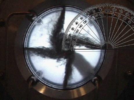
19 10 Spread Angle Spread angle is the angle at which the aluminum particle cloud initially exits the injection site. It is measured from one side of the aluminum cloud to the other, an example of which is shown in Figure 2-4. Analyzing the videos for spread angle was accomplished using screen shots of the video and an on-screen protractor overlay. Spread angles varied from 5 to 50, and are found to vary with the injector type, angle of injection, total mass flow rate, and velocity of injection. To determine the spread angle, a frame that best represented the steady-state flow of the test was used. In the case that this was not possible, an ensemble average of multiple frames was used. A summary of the spread angles is given in Table 2-3, and figures from which the spread angles were extracted can be seen in Appendix D. The radial injection angle was determined from recorded test data and programed into each flow model appropriately.

20 11 Table 2-3. Particle Spread Angles Determined from Analysis of Test Data Test Number Spread Angle (degrees) Test Number Spread Angle (degrees) Test Number Spread Angle (degrees) Test Number b Spread Angle (degrees) NA* NA* NA* NA* NA* NA* NA* Figure 2-4. Screenshot used to determine particle spread angle in Test 7-1

21 12 Particle Size The nominal particle size used in these tests was 10 µm. However, to further understand the flow properties of the aluminum particles in the fuel-feed system the aluminum powder batches were subjected to laser diffraction particle sizing analysis. The laser diffraction method measured the particle sizes by determining the amount of light scattered by individual aluminum particles. The particle size D N includes all of the particles from zero up to the tabulated size required to occupy N% of the powder volume. The table in Appendix E includes the diameters for the different particle batches used in the flow visualization test, while Table 4 indicates the particle batch used in each test. Test Number Table 2-4. Powder Batches Used In Flow Visualization Powder Batch Number Test Number Powder Batch Number Test Number Powder Batch Number Test Number Powder Batch Number 1-1 no data sheet 2-8 no data sheet no data sheet 2-9 no data sheet no data sheet no data sheet 3-2 not listed no data sheet no data sheet no data sheet 3-5 no data sheet 5-5 not listed no data sheet not listed no data sheet not listed no data sheet not listed no data sheet not listed no data sheet no data sheet no data sheet no data sheet 4-5 no data sheet

22 13 Recirculation Radius The recirculation radius is the distance from the center of the chamber exit at which aluminum particles continue to orbit inside the chamber before exiting. A frame representative of the steady-state of the flow is used to measure the recirculation radius, as seen in Figure 2-5. The measured recirculation radii for all experimental tests with video are listed in Table 2-5. An average particle will travel slightly under one full rotation around the chamber before exiting, as illustrated in Figure 2-6. Figure 2-5. Example of a measured recirculation radius Figure 2-6. Example particle path from injection to exhaust

23 14 Table 2-5. Recirculation Radius Test number Recirculation Radius (cm) Test number Recirculation Radius (cm) Test number Recirculation Radius (cm) Test number Recirculation Radius (cm) no video 4-6 no video no video 4-7 no video no video no video no video no video no video no video no video no video no video

24 15 Chapter 3 Description of Models Drag Model The drag coefficient, CD, is used to quantify the drag on an object in a fluid flow, and includes two main components: surface friction and form drag. It is used to find the drag force (F d ), as shown in Equation (4). Because CD is a function of flow speed, object geometry, fluid viscosity, and fluid density, it is a function of Reynolds number. For compressible flow, the Mach number is also a factor, but that dependence can be regarded as negligible for low Mach numbers. For the purposes of this study, aluminum particles will be modeled as spheres with characteristic length D (diameter) and reference area A = πr 2 (r = D/2). The effect of densely laden clouds on drag coefficient is not explored, although it could change the drag coefficient depending on concentration of aluminum particles. A useful drag model will provide an analytical description of the relationship between Reynolds number and drag coefficient over the range of Reynolds number encountered. For small Reynolds numbers, a Stokes Law approximation of 24/Re is a good approximation of the drag coefficient, but this approximation diverges from experimental data (Figure 3-1) significantly at Reynolds values above ten and requires modification to remain accurate at high Re (3). Before the flow becomes fully turbulent, (Re < 1x10 5 ), a five-parameter correlation by Cheng (Equation (5)) provides a theoretical analysis with only a 2.469% average error (see Table 3-1) (4).This correlation is compared to seven other correlations that predicted the entire subcritical region and Equation (5) was shown to give the best representation of the effect of Reynolds number on coefficient of drag when compared to experimental data (Figure 3-1) (4). A simpler model used in an older version of FLUENT (5), the Cheng model, and Alexander and Morsi (6) are compared to

25 16 the same set of experimental data in Figures 3-2 through 3-4 (7). Ultimately we implemented Alexander and Morsi (Figure 3-4) because of the small differences between models in the range of Reynolds numbers we used (~1*10^5), and the fact that it was hardwired into one of the FLOW3D models. (4) (5) Figure 3-1. Equation 5 vs. Experiment (4)

26 17 Table 3-1. Relative accuracies of different drag model correlations Investigator Prediction Average Error from Experimental Data (%) Cheng (4) Clift et al. (8) Brown and Lawler (9) Turton and Levenspiel (10) Clift and Fauvin (8) Concha and Barrientos (11) Flemmer and Banks (7) Almedeij (12) 4.762

27 Cd = 24/Re*(1+Re^(2/3)/6) Experimental Figure 3-2. Fluent model versus experimental data Fluent Model (5): Re<1000: CD = 24/Re*(1+Re^(2/3)/6) Re>1000: CD = Experimental Figure 3-3. Cheng model versus experimental data Cheng Model (4): Re<2.35E5: CD = 24/Re*(1+0.27*Re)^ *(1-exp(-0.04*Re^.38)) 2.35E5<Re<3.55E5 CD = ( /Re)^3.5 (Wittenstein modification)* 3.55E5<Re CD = Re^(1/3)/700 (Wittenstein modification)* *Added relationship to account for Reynolds numbers over 2.35E5

28 Experimental MORSI Figure 3-4. Morsi and Alexander model versus experimental data Morsi and Alexander Model (6): Re<.1 CD = 24/Re.1<Re<1.0: CD = 22.73/Re+.0903/Re^ <Re<10.0 CD = /Re-3,8889/Re^ <Re<100.0 CD = 46.5/Re-116/Re^ <Re< CD = 98.33/Re-2778/Re^ <Re< CD = /Re-4750/Re^ <Re< CD = /Re /Re^ <Re< CD = /Re /Re^

29 20 Eulerian Models The program used to model the flow is FLOW3D, a CFD code that solves the Navier- Stokes equations using a pressure-based algorithm based on SIMPLE (Semi-Implicit Method for Pressure Linked Equations), and uses a K-Epsilon model for turbulence (13). Two Eulerian approaches to modeling are the single-phase and the multi-phase model. Although the multiphase model calculates the conservation equations for each species separately, multi-phase models often experience instability that single-phase models do not (14). The differencing method used in the single-phase models below is CONDIF, a differencing scheme which uses a central differencing scheme where possible, and an upwind differencing scheme where nonphysical overshoot would occur. The multiphase models used CCCT differencing, which is a differencing scheme based on QUICK with modifications at the boundaries (1). Both QUICK and CONDIF are second order differencing schemes programed into the CFDS-FLOW3D software. Single-Phase Model In the single-phase approach, a single fluid is modeled inside the chamber, consisting of three species: nitrogen, argon, and the solid particles. Local fluid properties, including density, thermal conductivity, specific heat, and turbulence quantities are mixture-averaged quantities, determined by the local concentration of each species and its associated properties. A single set of compressible conservation equations is solved using SIMPLE, described below, with the relative drift between species caused by their different densities and drag forces being determined by calculating a local drift flux as described by Cor and Miller (2). This drift flux becomes a source term in the species, momentum and energy conservation equations. Equations (6)-(9) show how the drift flux term V d,p, defined below, becomes a source term in the continuity, momentum,

30 21 and energy equations (2). In each of the equations below, m stands for mixture, p stands for particle, and g stands for gas. The symbol α represents volume fraction and τ represents viscous and turbulent stresses. The mixture density ρm is calculated from ρ g, and ρ m, with ρ g coming from the ideal gas law and ρm a constant, using Equation (2). Velocities u r, v r, and w r all are solved for by finding acceleration using central differencing and then solving Equation (10) (2). ({ [ ] }) (10)

31 22 Multi-phase Model In the multi-phase version, the particles and gas are treated separately as two different fluids. The particles are now in essence a separate pseudo-fluid, with its own unique set of thermodynamic properties such as pressure and viscosity, an additional property of volume fraction, and its own momentum as well. For each fluid, the full sets of incompressible conservation equations are solved for individually, with source terms in the momentum equations accounting for the drag force acting between the two phases. To do this, the IPSA (InterPhase Slip Algorithm) (15) is used, which is an extension of the SIMPLE algorithm, an iterative method to solve the Navier-stokes equations (16). The steps used to solve the SIMPLE equation are shown in Figure 3-5. Figure 3-5. Steps involved in the SIMPLE algorithm (17) For both the single-phase and multi-phase models, the variable drag force acting on a particle is determined from Equation (4). CD is determined using the model of Morsi and Alexander, described in Chapter 3 Part 1, or alternatively using a constant CD value of A CD value of 0.44 is found to be accurate over the Reynolds number range of 10 3 to It is

32 23 hypothesized that this drag model may be appropriate for turbulent flows, which are being modeled in this study. Three Particle Size Model The three-particle-size model is a modification of the single-phase model to account for the variation in diameters of each aluminum particle batch. Only one set of continuity equations is used, but the force on each species is determined using the separate diameters, changing the relative drift flux. Instead of the aluminum particles being modeled as a 10 micrometer diameter species, they are instead modeled as three species of varying diameters. In the initial test modeled, 3-1, the diameters used are based on Appendix E, with 30% of the aluminum flow modeled as 9.38 μm, 40% modeled as μm, and 30% modeled as μm. The diameter of the particles affects the drag force calculation in Equation (4). Only test 3-1 was modeled using varying diameters, but future use with this model is possible. Lagrangian Model In Lagrangian analysis, the gas phase is still treated via an Eulerian analysis, but the trajectories of the particles are calculated based on a transient analysis of an individual particle as it flows through the gas field. The gas field is based on the single-phase model, and uses the same equations and methods listed previously. The local conditions of the gas as the particles travel through them determine the forces acting on the particle that alter its trajectory. The particle in turn produces an opposite force acting on the gas, and these particle forces are treated as source terms in the momentum conservation equations of the Eulerian gas. A Runge-Kutta method is used to advance the particles through time until they exit the computational domain of

33 24 the model (18). Due to computational restrictions, each aluminum injector is treated as four particle injection points, as seen in Figure 3-5, and the mass flow rate (A*v*ρ) from Equation (4) is modified to reflect the larger mass flow rate that each particle represents. Figure 3-6. Injection points used in the Lagrangian model at one of the four aluminum injectors Transient Model In this analysis, the multi-phase model is used to simulate the flow as it develops over time. This model will be used in future modeling of the high-speed video tests, as in these test videos the initial flow development can be seen more clearly. The normal-speed video tests use a 30-frame-per-second camera which only catches approximately four frames of the flow before it is fully developed, while the high speed 1800-frame-per-second camera can catch upwards of 200 frames before the flow becomes fully developed. The transient model uses a backward Euler method to advance in time, as seen in Equation (11) (18).

34 25 (11)

35 26 Computational Grid The computational grid contained 25 points in the axial direction, 35 points in the radial direction, and 186 points in the azimuthal direction, for a total of 162,750 points. The grid spans 360 degrees, allowing the modeling of up to four aluminum injector points, as well as 16 mixing injectors. Originally, the grid was one-quarter symmetry to preserve computational time, but a full-scale grid was created for more accurate modeling by mirroring the existing grid across the horizontal and vertical axis. All of the distribution and shroud injectors, shown in Figure 2-1, are approximated as continuous injectors spanning the distance between aluminum/mixing injection locations. The grid can be seen in Figure 3-6 below, with red representing area of nitrogen injection. Figure 3-7. Computational grid with nitrogen injection locations in red

36 27 Chapter 4 Test Analysis and Modeling Results Quantitative Data Comparison Quantitative comparisons between the modeling and test data have been made for the recirculation radius and the injection spread angle. The recirculation radius is the distance from the center of the chamber that the particles continue to orbit around the exit before leaving the chamber, as seen in Figure 4-1. The injection spread angle is a measurement of the spread of the flow as it enters the chamber; it is measured from one side of the flow to the other as the flow moves towards the center of the chamber, as also shown in Figure 4-1. For the model results, recirculation radius is determined by plotting mass fraction contours at a very low level (from.001 to.05, the lowest levels where flowing aluminum was distinguishable from resident aluminum in the chamber) to find the extent of the particle orbit around the chamber exit hole. An example of this is seen in Figure 4-2. The exact mass fraction level at which aluminum particles were visible in the chamber cannot be determined from the video data, therefore multiple levels of mass fractions from the CFD models are compared to experimental data. Figure 4-1. Recirculation radius and spread angle of Test 3-1

37 28 Figure 4-2. Typical modeling result using a minimum mass fraction contour of.001 for determining recirculation radius

38 29 Test 3-1 Test 3.1 was the first test chosen for evaluating the different CFD models, as it had the best flow with four injectors. This was the baseline case used in evaluating flow mixing in the Loki program as well. Using the flow rates, pressures, and injection geometries of Test 3-1, the three different CFD modeling techniques were used to simulate the flow in the chamber. The conditions for Test 3-1 can be found in Table 4-1 below. Each set of figures (Figures 4-3 to 4-8) includes a slice of the model results from the center of the chamber, as well as a contour view from the back window, which is the same view as the experimental videos. Because the viewing location of the contour slice and the view of iso-surface are different, the mass fractions are not the same, although the color scale of each view represents the same mass fractions. Figures 4-3 and 4-4 show the modeling results using the single-phase model. Figures 4-5 and 4-6 show the modeling results using the multi-phase model. Figures 4-3 and 4-5 were generated using the CD correlation of Alexander and Morsi drag, while Figures 4-4 and 4-6 were generated using a constant CD value of The use of the correlation of Morsi and Alexander appears to underpredict the recirculation radius relative to the use of the constant CD value of Figure 4-6, which shows the multi-phase constant CD model, best predicts the flow based on visual inspection, followed by the single-phase constant CD model. Figure 4-7 shows the modeling results using the Lagrangian model with the correlation of Morsi and Alexander, while Figure 4-8 shows the Lagrangian modeling results using the constant value of CD of The lagrangian models could not capture the spread angle due to the low amount of particles modeled due to computational restrictions. The constant CD drag model better predicts the recirculation pattern seen at the exit of the chamber in the experimental video. Table 4-2 compares the qualitative results between each of the models and experimental data. Figures 4-9 and 4-10 show the threediameter models compared to the single phase model results of the same drag model. In these

39 cases, recirculation radius was very similar, but spread angle varied between the models. Further testing of the three diameter model is needed for verification of accuracy. 30 Table 4-1. Test 3-1 test conditions Aluminum Flow Rate (g/s) 36 Argon Carrier Gas Flow (g/s) 1.04 N2 Distribution Flow Rate (g/s) 72 N2 Chamber Shroud Flow Rate (g/s) 19 N2 Mixing Flow Rate (g/s) 7 Number of Aluminum/Argon Injectors 4 Number of Distribution Injectors 160 Number of Chamber Shroud Injectors 168 Number of Mixing Injectors 16 Aluminum/Argon Injector Area (cm^2).268 Distribution Area Per Injector (cm^2).195 Chamber Shroud Area Per Injector (cm^2) Mixing Flow Area Per Injector (cm^2).123

40 31 Figure 4-3. Calculated aluminum mass fraction contours using the single phase model with correlation of Morsi and Alexander, results superimposed over video frame from Test 3-1, and video frame from Test 3-1. Figure 4-4. Calculated aluminum mass fraction contours using the single phase model with constant drag coefficient, results superimposed over video frame from Test 3-1, and video frame from Test 3-1.

41 32 Figure 4-5. Calculated aluminum mass fraction contours using the multi-phase model with correlation of Morsi and Alexander, results superimposed over video frame from Test 3-1, and video frame from Test 3-1. Figure 4-6. Calculated aluminum mass fraction contours using the multi-phase model with constant drag coefficient, results superimposed over video frame from Test 3-1, and video frame from Test 3-1 Figure 4-7. Calculated aluminum particle trajectories using Lagrangian model with correlation of Morsi and Alexander plotted in full view, in close-up view at the exit, and video frame from Test 3-1.

42 33 Figure 4-8. Calculated aluminum particle trajectories using Lagrangian model with constant drag coefficient plotted in full view, in close-up view at the exit, and video frame from Test 3-1.

43 34 Figure 4-9. Three diameter constant CD results for test 3-1 compared to results with single diameter model. Bottom left figure is all three diameter particles combined.

44 35 Figure Three diameter variable CD results for test 3-1 compared to results with single diameter model. Bottom left figure is all three diameter particles combined.

45 36 Table 4-2. Test 3-1 Quantitative results and test data comparison Test 3-1 Spread Angle (degrees) Spread Angle % error Recirculation Radius (cm) Recirculation Radius % error Experimental Data Single Phase CD = % % Singe Phase CD = variable % % Mphase CD = % % Mphase CD = variable % % Lagrangian CD =.44 NA NA % Lagrangian CD = variable NA NA Three Diameter CD = % Three Diameter CD = variable % % 46.47% 62.65%

46 37 Test 2-8 Test 2-8 was selected for modeling to test the effect of using a different aluminum flow rate into the vortex chamber. The test conditions can be seen in Table 4-3, showing the same geometry as test 3-1. Compared to test 3-1, test 2-8 has an increased aluminum and argon flow rate, which increases the velocity of the flow at the injection point. Slight differences in nitrogen injector flow rates are also seen, but these are much smaller than the differences in aluminum/argon flow rates. Figures 4-11 and 4-12 show the modeling results using the singlephase model. Figures 4-13 and 4-14 show the modeling results using the multi-phase model. Figure 4-11 and 4-13 were generated using the CD correlation of Alexander and Morsi drag, while Figures 4-12 and 4-14 were generated using a constant CD value of Once again, the multi-phase constant CD represents the experimental flow best based on visual inspection, as seen in Figure Figures 4-11 and 4-13 show the variable CD under-predicting recirculation radius, as was seen in test 3-1. The multi-phase models predict a higher recirculation radius for test 2-8, consistent with experimental results, while the single-phase models predict slightly smaller recirculation radius. Table 4-3. Test 2-8 conditions Aluminum Flow Rate (g/s) 45 Argon Carrier Gas Flow (g/s) N2 Distribution Flow Rate (g/s) 74 N2 Chamber Shroud Flow Rate (g/s) 19 N2 Mixing Flow Rate (g/s) 7 Number of Aluminum/Argon Injectors 4 Number of Distribution Injectors 160 Number of Chamber Shroud Injectors 168 Number of Mixing Injectors 16 Aluminum/Argon Injector Area (cm^2).268 Distribution Area Per Injector (cm^2).195 Chamber Shroud Area Per Injector (cm^2) Mixing Flow Area Per Injector (cm^2).123

47 38 Figure Calculated aluminum mass fraction contours using the single phase model with correlation of Morsi and Alexander, results superimposed over video frame from Test 2-8, and video frame from Test 2-8. Figure Calculated aluminum mass fraction contours using the single phase model with constant drag coefficient, results superimposed over video frame from Test 2-8, and video frame from Test 2-8. Figure Calculated aluminum mass fraction contours using the multi-phase model with correlation of Morsi and Alexander, results superimposed over video frame from Test 2-8, and video frame from Test 2-8.

48 39 Figure Calculated aluminum mass fraction contours using the multi-phase model with constant drag coefficient, results superimposed over video frame from Test 2-8, and video frame from Test 2-8. Figure Calculated aluminum particle trajectories using Lagrangian model with correlation of Morsi and Alexander plotted in full view, in close-up view at the exit, and video frame from Test 2-8 Figure Calculated aluminum particle trajectories using Lagrangian model with constant drag coefficient plotted in full view, in close-up view at the exit, and video frame from Test 2-8.

49 40 Table 4-4. Test 2-8 Quantitative Modeling and Test Data Comparison Test 2-8 Spread Angle (degrees) Spread Angle % Error Recirculation Radius (cm) Experimental Data Recirculation Radius % Error Single Phase CD = % % Singe Phase CD = variable % % Mphase CD = % % Mphase CD = variable % % Lagrangian CD =.44 NA NA % Lagrangian CD = variable NA NA %

50 41 Test 5-1 Test 5-1 is a single-injector case which uses the same injector geometry as the first two tests (3-1 and 2-8). The number of mixing, chamber shroud, and distribution nitrogen injectors remains constant, as can be seen in Table 4-5. In this test, there is very little recirculation; this is predicted by each model. Figures 4-17 and 4-18 show the modeling results using the single-phase model. Figures 4-19 and 4-21 show the modeling results using the multi-phase model. Figure 4-17 and 4-19 were generated using the CD correlation of Alexander and Morsi drag, while Figures 4-18 and 4-20 were generated using a constant CD value of Figure 4-20, the results for the multi-phase model with constant CD, predicts the highest recirculation radius, while the multiphase variable Morsi and Alexander model predicts the smallest recirculation radius. Visually, the single-phase constant CD model in Figure 4-18 has the best representation of the experimental video. Table 4-5. Test conditions for test 5-1 Aluminum Flow Rate (g/s) 14 Argon Carrier Gas Flow (g/s).36 N2 Distribution Flow Rate (g/s) 73 N2 Chamber Shroud Flow Rate (g/s) 20 N2 Mixing Flow Rate (g/s) 7 Number of Aluminum/Argon Injectors 1 Number of Distribution Injectors 160 Number of Chamber Shroud Injectors 168 Number of Mixing Injectors 16 Aluminum/Argon Injector Area (cm^2).268 Distribution Area Per Injector (cm^2).195 Chamber Shroud Area Per Injector (cm^2) Mixing Flow Area Per Injector (cm^2).123

51 42 Figure Calculated aluminum mass fraction contour using the single phase model with correlation of Morsi and Alexander, isosurface results superimposed over video frame from Test 5-1, and video frame from Test 5-1. Figure Calculated aluminum mass fraction contour using the single phase model with constant drag coefficient, isosurface results superimposed over video frame from Test 5-1, and video frame from Test 5-1. Figure Calculated aluminum mass fraction contour using the multi-phase model with correlation of Morsi and Alexander, isosurface results superimposed over video from Test 5-1, and video frame from Test 5-1

52 43 Figure Calculated aluminum mass fraction contour using the multi-phase model with constant drag coefficient, isosurface results superimposed over video from Test 5-1, and video frame from Test 5-1. Figure Calculated aluminum particle path using the Lagrangian model with constant drag coefficient, results superimposed over video frame from Test 5-1, and video frame from Test 5-1. Figure Calculated aluminum particle path using the Lagrangian model with correlation of Morsi and Alexander, results superimposed over video frame from Test 5-1, and video frame from Test 5-1

53 44 Table 4-6. Test 5-1 Quantitative Modeling and Test Data Comparison Spread Angle Test 5.1 (degrees) Experimental Data 30 Spread Angle % Error Single Phase CD = % Singe Phase CD = variable % Mphase CD = % Mphase CD = variable % Lagrangian CD =.44 Lagrangian CD = variable Recirculation Radius (cm) NA NA 0.00 NA NA 0.00 Recirculation Radius % Error % 32.35% % 40.20% % %

54 45 Test 5-9 Test 5-9 is a two-injector case which uses the same injector geometry and number of nitrogen injectors as the previous cases. We chose this test to evaluate a two-injector test case, and also used it for initial testing of a transient model for future analysis of test Series 7, the highspeed videos. Figures 4-23 and 4-24 show the modeling results using the single-phase model. Figures 4-25 and 4-26 show the modelng results using the multi-phase model. Figure 4-23 and 4-25 were generated using the CD correlation of Alexander and Morsi drag, while Figures 4-24 and 4-26 were generated using a constant CD value of Once again, the constant CD multi-phase model is the most similar visually to the experimental video, as seen in Figure It also has the best prediction of recirculation radius, although the variable multi-phase model has the best prediction of spread angle, as seen in Table 4-8. The initial transient modeling, seen in Figure 4-27, looks promising as the time for the experimental flow to reach steady state is on the same order as the model. For better comparison, an experimental test with high-speed video footage must be modeled. Table 4-7. Test conditions for test 5-9 Aluminum Flow Rate (g/s) 14 Argon Carrier Gas Flow (g/s) 2.99 N2 Distribution Flow Rate (g/s) 70 N2 Chamber Shroud Flow Rate (g/s) 19 N2 Mixing Flow Rate (g/s) 8 Number of Aluminum/Argon Injectors 2 Number of Distribution Injectors 160 Number of Chamber Shroud Injectors 168 Number of Mixing Injectors 16 Aluminum/Argon Injector Area (cm^2).268 Distribution Area Per Injector (cm^2).195 Chamber Shroud Area Per Injector (cm^2) Mixing Flow Area Per Injector (cm^2).123

55 46 Figure Calculated aluminum mass fraction contour using the single phase model with correlation of Morsi and Alexander, isosurface results superimposed over video frame from Test 5-9, and video frame from Test 5-9. Figure Calculated aluminum mass fraction contour using the single phase model with constant drag coefficient, isosurface results superimposed over video frame from Test 5-9, and video frame from Test 5-9. Figure Calculated aluminum mass fraction contour using the multi-phase model with correlation of Morsi and Alexander, isosurface results superimposed over video frame from Test 5-9, and video frame from Test 5-9.

56 47 Figure Calculated aluminum mass fraction contour using the multi-phase model with constant drag coefficient, isosurface results superimposed over video frame from Test 5-9, and video frame from Test 5-9. Figure Calculated aluminum mass fraction contour using the transient multi-phase model with correlation of Morsi and Alexander from t=.002 to t =.11 seconds

57 48 Table 4-8. Quantifiable Test Results from Test 5-9 Spread Angle Spread Angle % Recirculation Radius Test 5.1 (degrees) Error (cm) Experimental Data Recirculation Radius % Error Single Phase CD = % % Singe Phase CD = variable % % Mphase CD = % % Mphase CD = variable % %

58 49 Chapter 5 Conclusion Each of the models tested (single-phase, multi-phase, and Lagrangian) have yielded results which at least in some ways best represent the experimental data. Considerations when choosing between the three models are robustness, computational costs, and accuracy. The Lagrangian model did not show spread angle or recirculation radius due to the limited number of particles modeled, although it does model an average particle path in the center of the flow. This means that the accuracy in comparison to both the spread angle and recirculation radius was not possible to compare. The multi-phase and single-phase models were the most stable and robust, while the Lagrangian model had problems with numerical stability. The Lagrangian method had by far the most computational failures and convergence was rare, leading to this model being left out of Test 5-9 modeling. Computationally, both the multi-phase and single-phase models took approximately the same amount of computational time to complete, while the Lagrangian method took the most processor time to run. The most important among the three qualities used to rank the models is relative accuracy. The accuracy of the model is quantified in two ways: first, by spread angle and recirculation, and second by qualitatively evaluating the model s similarity to videos of the experiments. The accuracy of the single-phase and multi-phase models was similar, but the multiphase model predicted spread angle and recirculation radius faster, more consistently (in terms of stability), and with only slightly less accuracy than the single-phase model (Table 5-1 and 5-2). As the graphs in Figure 5-1 and 5-2 show, each model using a constant coefficient of drag predicts a low of inches absolute average error in recirculation radius, while the Alexander and Morsi model predicts a low of inches. Although accuracy of the models quantitatively was similar, the single-phase model allows for differing particle sizes, which

59 50 allows us to take into account the particle batch sizes available in Appendix E. The multi-phase model however can be used to run transient versions of the models. A second consideration in modeling is the drag model. The variable drag model and constant-coefficient drag model were both used for each of the three modeling programs for each test. The variable drag model is based on Morsi and Alexander (6) as seen in the description of the variable drag model earlier in the thesis. Neither of these tests differed in terms of robustness or computational costs, but they did differ in results. The constant-coefficient drag model, which used a CD significantly lower than the CD obtained using the variable-coefficient of drag model, tended to have more mass spread out through the recirculation radius; more of the aluminum recirculated through the chamber. The spread angle using the constant CD has an average absolute error of approximately 4.35 degrees, which was worse than the variable absolute average error. The variable coefficient of drag model tended to have a smaller recirculation radius at higher mass fractions compared to the constant coefficient of drag model, indicating less mass recirculating around the chamber. The spread angle measurement was most accurate for the variable CD, multi-phase model, yet least accurate for the constant CD, multi-phase model. Table 5-1 shows both average and absolute average error in recirculation radius compared to experimental data. It shows the recirculation rate measured at different minimum mass fraction levels:.05,.01,.005, and.001. These values are close to the minimum mass fraction at which we can differentiate between flowing aluminum mass and resident gas in the chamber, with each lower mass fraction predicting a higher recirculation radius. Table 5-2 shows the absolute average error in spread angle of each model, with the multi-phase variable drag model being the most accurate model in this respect. Figure 5-1 and 5-2 are the graphs of the data from Table 5-1, making it easier to see how much error is present in each model in terms of recirculation radius.

60 51 Although it is very difficult to assess the amount of mass moving throughout the chamber, the constant CD model more reliably predicted the experimental recirculation radius and qualitatively resembled the experimental data more closely. Overall, the Morsi and Alexander drag model increased the accuracy in predicting spread angle, especially in the multi-phase model, but caused under prediction of recirculation radius in both single and multi-phase models. Table 5-1. Quantifiable recirculation test result comparison between tests, both average error (top) and absolute error (bottom) Mass Fraction Modeling versus experimental, average error (cm) Single-Phase Model Multi-Phase Model Constant CD Variable CD Constant CD Variable CD Modeling versus experimental, absolute average error (cm) Mass Single-Phase Model Multi-Phase Model fraction Constant CD Variable CD Constant CD Variable CD Table 5-2. Quantifiable spread angle result comparison between tests Average absolute difference in spread angle (degrees) Single Phase CD = Singe Phase CD = variable 5.5 Multi-phase CD = Multi-phase CD = variable 1.75

61 52 Average error 0.4 versus 0.2 experimental 0 (inches) Mass fraction level Single Constant Single Variable Multi Constant Multi Variable Figure 5-1. Test average recirculation radius error at four different minimum mass fraction levels Average absolute error versus experimental (inches) Single Constant Single Variable Multi Constant Multi Variable Mass fraction level Figure 5-2. Test average absolute recirculation radius error at four different minimum mass fraction levels

62 53 Future Work Moving forward with modeling will include further testing with current experimental data to cover all test cases available. It will also include modifying the constant coefficient of drag model as well as the variable drag model to better fit the experimental data in models already tested. Although a variety of conditions were tested using the selected tests, four test sets have yet to be modeled and can provide more comparison to experimental data. Moving forward with transient analysis, including accurate start up conditions, will allow comparison to test set seven high speed video which will enable modeling of the initial injection of particles into the vortex chamber. Further analysis of multiple particle size models will allow the effect of smaller or larger particle size batches to be seen in the flow of particles using Appendix E. Once further testing has been completed using the current experimental data and sufficient validation of the model has occurred, implementation into multi-phase model that includes chemical reactions, radiative heat transfer, and phase changing environments will enable further performance testing. Experimental data has already been gathered that will allow for comparison with future model testing, both with and without combustion.

63 54 Appendix A Flow Rates Test # Aluminum Flow Rate (g/s) Argon Carrier Gas Flow (g/s) N 2 Distribution Flow Rate (g/s) N 2 Chamber Shroud Flow Rate (g/s) N 2 Mixing Flow Rate (g/s) Total Gas Flow Rate (g/s) falling falling rising rising falling measured 218 measured 218 measured

64 55 Test # Aluminum Flow Rate (g/s) Argon Carrier Gas Flow (g/s) N 2 Distribution Flow Rate (g/s) N 2 Chamber Shroud Flow Rate (g/s) N 2 Mixing Flow Rate (g/s) Total Gas Flow Rate (g/s) falling falling b rising

65 Appendix B Velocity Calculations Fuel/Carrier Gas Test # Total Aluminum Mass Flow Rate (g/s) Aluminum Mass Flow Rate per nozzle (g/s) Number of Aluminum Injectors Aluminum Injector Area (cm^2) Total Argon Mass Flow Rate (g/s) Argon Flow Rate Per Injector (g/s) Pressure (kpa) Argon Density (kg/m^3) Aluminum Density (kg/m^3) Injection Density (kg/m^3) Injection Velocity (m/s) * *

66 Test # Total Aluminum Mass Flow Rate (g/s) Aluminum Mass Flow Rate per nozzle (g/s) Number of Aluminum Injectors Aluminum Injector Area (cm^2) Total Argon Mass Flow Rate (g/s) Argon Flow Rate Per Injector (g/s) Pressure (kpa) Argon Density (kg/m^3) Aluminum Density (kg/m^3) Injection Density (kg/m^3) 57 Injection Velocity (m/s) * b

67 Test # Total Aluminum Mass Flow Rate (g/s) Aluminum Mass Flow Rate per nozzle (g/s) Number of Aluminum Injectors Aluminum Injector Area (cm^2) Total Argon Mass Flow Rate (g/s) Argon Flow Rate Per Injector (g/s) Pressure (kpa) Argon Density (kg/m^3) Aluminum Density (kg/m^3) Injection Density (kg/m^3) 58 Injection Velocity (m/s) \

68 Appendix C 59 Nitrogen Velocities Test Number N 2 Density (kg/m^3) Distribution. Area Per Injector (mm^2) Chamber Shroud Area Per Injector (mm^2) Mixing Flow Area Per Injector (mm^2) Number of Distribution Injectors Number of Chamber Shroud Injectors Number of Mixing Injectors Distribution Velocity (m/s) Chamber Shroud Velocity (m/s) Mixing Velocity (m/s)

69 60 Test Number b N 2 Density (kg/m^3) Distribution. Area Per Injector (mm^2) Chamber Shroud Area Per Injector (mm^2) Mixing Flow Area Per Injector (mm^2) Number of Distribution Injectors Number of Chamber Shroud Injectors Number of Mixing Injectors Distribution Velocity (m/s) Chamber Shroud Velocity (m/s) Mixing Velocity (m/s) NA NA NA NA NA NA NA NA

70 61 Test Number N 2 Density (kg/m^3) Distribution. Area Per Injector (mm^2) Chamber Shroud Area Per Injector (mm^2) Mixing Flow Area Per Injector (mm^2) Number of Distribution Injectors Number of Chamber Shroud Injectors Number of Mixing Injectors Distribution Velocity (m/s) Chamber Shroud Velocity (m/s) Mixing Velocity (m/s)

71 Appendix D 62 Spread Angle Screenshots Test 1-1 Test 1-2 Test 1-3 Test 1-4 Test 1-5 Test 1-6 Test 2-2 Test 2-4 Test 2-7 Test 2-8

72 63 Test 3-1 Test 3-2 Test 3-3 Test 3-4 Test 3-5 Test 3-6 Test 3-7 Test 4-1 Test 4-3 Test 5-1 Test 5-2

73 64 Test 5-3 Test 5-4 Test 5-4b Test 5-5 Test 5-6 Test 5-9 Test 5-10 Test 6-2 Test 6-3 Test 6-4 Test 6-5 Test 6-6

74 65 Test 6-7 Test 6-8 Test 6-9 Test 6-10 Test 6-11 Test 7-1 Test 7-2 Test 7-3

75 Appendix E 66 Particle Distribution Size

76 67