Spatial track: motion modeling
|
|
|
- Tyrone Hamilton
- 5 years ago
- Views:
Transcription
1 Spatial track: motion modeling Virginio Cantoni Computer Vision and Multimedia Lab Università di Pavia Via A. Ferrata 1, Pavia 1

2 Comparison between Motion and Stereo Analysis Stereo: two or more frames baseline Motion: N frames time The baseline is usually larger in stereo than in motion: Motion disparities tend to be smaller Stereo images are taken at the same time: Motion disparities can be due to scene motion There can be more than one transformation between frames 2

3 Ill-posed problem As an illustrative example, positively using this limitation to attract attention, consider the barber-shop banner usually displayed outdoors in many countries. Typically, a rotation movement of a 3-coloured striped pattern on a cylinder, perceptually suggests that the whole pattern is translated vertically upwards. A rotational movement of a homogeneous sphere cannot be perceived, meanwhile a still sphere is perceived rotating if the source of light is rotating around. 3
4 Motion versus stereo analysis: correspondences Small displacements differential algorithms based on gradients in space and time dense correspondence estimates most common with video Large displacements matching algorithms based on correlation or features sparse correspondence estimates most common with multiple cameras/stereo Correspondence types point correspondences line correspondences curve correspondences region correspondences
5 Why Multitude of Formulations? How is the camera moving? the camera can be stationary execute simple translational motion undergo general motion with both translation and rotation How many moving objects are there? the object(s) can be stationary execute simple 2D motion parallel to the image plane undergo general motion with both 3D translation and rotation Which directions are they moving in? How fast are they moving? Can we recognize their type of motion (e.g. walking, running, etc.)? The camera motion may be known or unknown The shape of the object may be known or unknown The motion of the object may be known or unknown etc. etc.... 5
6 Classes of Techniques Feature-based methods extract visual features (corners, textured areas) and track them sparse motion fields, but possibly robust tracking suitable especially when image motion is large (10s of pixels) Direct-methods directly recover image motion from spatio-temporal image brightness variations global motion parameters directly recovered without an intermediate feature motion calculation dense motion fields, but more sensitive to appearance variations suitable for video and when image motion is small (< 10 pixels) Szeliski
7 Classes of Techniques and Motion Models Motion models exploit two different invariants: in the first one, peculiar object points are assumed to be recovered from one image to the next in the second all visible-point intensities are supposed to be maintained along time. Two different approaches of motion are distinguished, respectively named discrete or sparse and continuous or dense: motion via correspondence motion via local change In the first case corresponding points must be found on different successive images. Note that, in stereo vision, to evaluate the position in space, point correspondences must be similarly found from different images. In the second case, a simple local analysis on the whole image must be performed with the limitation that only one motion component may be detected, the one orthogonal to the image contour. 7
8 Global Flow Dominant motion in the image motion of all points in the scene motion of most of the points in the scene component of motion of all points in the scene Global motion is caused by motion of sensor (Egomotion) motion of a rigid scene Estimation of global motion can be used to image alignment (Registration) removing camera jitter tracking (by neglecting camera motion) video segmentation etc.
9 Motion Detection and Estimation in Literature Image differencing based on the thresholded difference of successive images difficult to reconstruct moving areas Background subtraction foreground objects result by calculating the difference between an image in the sequence and the background image (previously obtained) remaining task: determine the movement of these foreground objects between successive frames Block motion estimation calculates the motion vector between frames for sub-blocks of the image Pointwise motion estimation: Optical Flow

10 Motion Field (MF) The MF assigns a velocity vector to each pixel in the image. These velocities are INDUCED by the RELATIVE MOTION btw the camera and the 3D scene The MF can be thought as the projection of the 3D velocities on the image plane. Examples of MF: Forward motion Rotation Horizontal translation Closer objects appear to move faster!! 10
11 Occlusion occlusion disocclusion shear Multiple motions within a finite region.
12 Forms of motion Translation at constant distance from the observer. Set of parallel motion vectors. Translation in depth relative to the observer. Set of vectors having common focus of expansion. Rotation at constant distance from view axis. Set of concentric motion vectors. Rotation of planar object perpendicular to the view axis. One or more sets of vectors starting from straight line segments.
13 Motion field and parallax P(t) is a moving 3D point Velocity of scene point: V = dp/dt P(t) V P(t+dt) p(t) = (x(t),y(t)) is the projection of P in the image Apparent velocity v in the image: given by components v x = dx/dt and v y = dy/dt These components are known as the MF of the image p(t) v p(t+dt)
14 Motion field V ( Vx, Vy, VZ ) p f P Z P(t) V P(t+dt) To find image velocity v, differentiate p with respect to t (using quotient rule): v f ZV VzP 2 Z Image motion is a function of both the 3D motion (V) and the depth of the 3D point (Z) p(t) v p(t+dt) Quotient rule: D(h/g) = (g h g h)/g 2
15 Preliminaries for motion analysis If A or B are moving objects with velocity components v x, v y, v z in 3D space, the corresponding velocity of the A or B image points, may be computed as follows: f A O B Image plane X Y O X The object speed in the scene is not known a-priori so that it must be estimated by the detected movement of the object projection on the image. Unfortunately, this problem is ill-posed since it is seldom possible to compute the object speed in space only knowing the planar displacement of its projections. Y B Z A 16


, or to some scene components, as cars in a")

16 Motion modeling: egomotion In many applications, a significant feature of the scene to be analyzed is the movement of some objects during a time interval. Such apparent movements may be due either to the image sensor, as in an airplane photographic campaign (egomotion), or to some scene components, as cars in a road scenario or both. First, egomotion is introduced and compensated next the camera is assumed to remain still for, leading back to the former analysis. 19
17 Egomotion the optical flow is istrumental at evaluating the shape and position of still components from their apparent motion due to the camera movement (egomotion). The sketch shows a camera downwards shift along the Z axis. Thanks to the relativity of perception it is equivalent to assume that the camera is still and the scene moves in the opposite direction along the Z axis. In this way, while the P point belonging to the ZY plane moves vertically down by P, its corresponding image point P moves along the Y axis by Y. Considering the triangle similarity: Y f Y Z and dy Y d so that the distance Z may be derived considering that dz is the known motion of the camera and (Y, dy) is determined from the image: Z Z Z Z d dy Y P DP Y f Z O Y DY 20

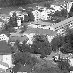
18 Motion field due to camera motion Length of flow vectors inversely proportional to depth Z of 3d point points closer to the camera move more quickly across the image plane Figure from Michael Black, Ph.D. Thesis
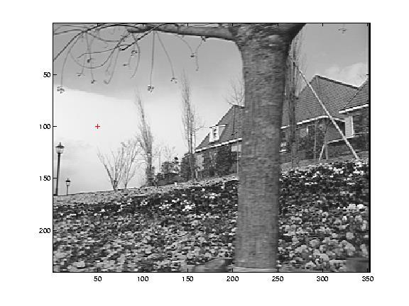
 could be estimated: the displacement dy with respect to the focus of expansion has the same relationship as the displacement along the Z axis with respect to the")
19 Egomotion: collision time The apparent movements are radial centered on the focus of expansion (FOE). A collision time (camera/object) could be estimated: the displacement dy with respect to the focus of expansion has the same relationship as the displacement along the Z axis with respect to the focal plane. For a camera having general velocity with components u, v and w respectively along the X, Y and Z axis, the generic object point Xo, Yo, Zo will be displaced on the image as: In order to compute the coordinates of the final/original destination of the moving point we may evaluate these for t= ± so obtaining the focus of expansion/contraction coordinates: and consequently the collision time. XO ut X f ; Y f Z wt O Y Z u v XFOE f ; YFOE f w w O O vt wt 22
20 Camera and egomotion The egomotion makes all still objects in the scene to verify the same motion model defined by three translations T and three rotations. Conversely, mobile obstacles pop out as not resorting to the former dominating model. Under such assumptions, the following classical equations hold: y Ω y Y R O T y P V ft xt xy x2 u X Z t, ur X 1 Y y Z f f Z ft yt xy y2 v Y Z t, vr Y 1 X x Z f f Z T w u, v u u, v v where t r t r stands for the 2-D velocity vector of the pixel under the focal length f. T Z T z Ω z z o v r p x T x Ω x X 23
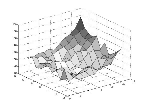
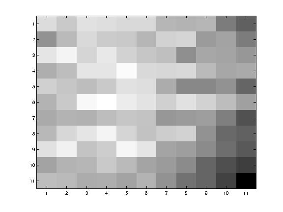
21 Coherent Motion Possibly Gaussian

22 From egomotion toward object speed Detected speeed Average speed Deviation due to the weighted object speed 25

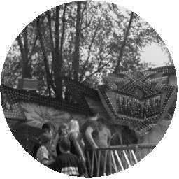
23 Motion via correspondences Even impoverished motion data can evoke a strong percept 30 points 10 points Normally, peculiar points on the first image are located so as to search their corresponding points on the second image. As in the triangulation for stereovision, there is no guarantee that such corresponding points exist and the new point of view may not include such points, moved out of the field of view. The object is first considered as a rigid one and therefore without plastic distortion and the background is regarded as stationary. In order to reduce the computational cost, the number of points is limited to the truly characteristic ones. Similarly to the epipolar segment for stereovision, the corresponding points are searched in a restricted area determined by a few heuristics. Primal sketch: locate the position of a pixel in the current image having similarity and the shortest Euclidean distance with respect to a point in the previous frame. 26


24 Patch Matching Where did each pixel in image 1 go to in image 2
25 Local Patch Analysis How certain are the motion estimates? Szeliski


26 Patch matching (revisited) How do we determine correspondences? block matching or SSD (sum squared differences) 29
27 Correlation Window Size Small windows lead to more false matches Large windows are better this way, but neighboring flow vectors will be more correlated (since the template windows have more in common) flow resolution also lower (same reason) more expensive to compute Small windows are good for local search: more detailed and less smooth (and referring to noise?) Large windows good for global search: less detailed and smoother 30
28 Maximum velocity A generic central object point can be located in the successive frame within a circle with a radius equal to V max t, where V max is the highest possible velocity of such point: 31
29 Obstacles The previous circular field is also limited by existing obstacles and physical boundaries contained in the scene 32
30 Maximum acceleration An extrapolation can enable TRACKING the object point in successive frames. The velocity detected in the two previous frames may be exploited to foresee the future position of the object point (time filtering). Same as before, a displacement will be inside a circle of radius equal to ½ A max Dt 2 where A max is the maximum acceleration; 33
31 Consistent matching Object points do not likely coalesce into one single point of the following frame, leading to the so-called consistent matching criterion. The picture shows four identified points that force the correspondence of the fifth dark one 34
32 Common motion Common motion situation: once the motion of the neighbors has been identified, the dark point necessarily maps into a congruent position (the depicted case is an expansion centered in the figure window) 35
33 Flexible motion model motion model for a herd of points suggesting the most plausible displacement of the dark object point. 36

34 Motion global models Translation 3D rotation Affine Perspective 2 unknowns 3 unknowns 6 unknowns 8 unknowns
35 Traslation Translation 2 unknowns
36 Affine Affine 6 unknowns
37 Planar perspective Perspective 8 unknowns
38 Tracking as induction Make a measurement starting in the 0 th frame Then: assume you have an estimate at the 1 th frame, after the measurement step. Show that you can do prediction for the i+1th frame, and measurement for the i+1th frame. Run two filters, one moving forward, the other backward in time. Now combine state estimates It is possible to iterate: we can obtain a smoothed estimate by viewing the backward filter s prediction as yet another measurement for the forward filter 46
39 position position position Tracking Forward estimates time Combined forward-backward estimates time Backward estimates time 47
40 Problem definition: optical flow How to estimate pixel motion from image H to image I? Solve pixel correspondence problem given a pixel in H, look for nearby pixels of the same color in I Key assumptions color constancy: a point in H looks the same in I For grayscale images, this is brightness constancy small motion: points do not move very far This is called the optical flow problem
41 Brightness Constancy I ( x r, y s, t 1) I ( x, y, t ) 0 s u frame t+1 frame t 49
42 Motion via local change,,,, f x x y y t t f x y t x y f f f t t x y t V f f t f 2 2 x y 50
43 Optical flow: mathematical formulation Brightness constancy assumption: u dx dy I( x t, y t, t t) I( x, y, t) dt dt Optical flow constraint equation : dx dt di dt v I x dy dt dx dt I y I x dy dt I y I t I y 0 I y I t I t I x u I y v I t 0 I T u v It 1 equation in 2 unknowns 51
44 Motion undetactable The brightness constancy constraint I T u v I 0 t The component of the motion perpendicular to the gradient (i.e., parallel to the edge) cannot be measured If [u,v] satisfies the equation, so does [u+u, v+v ] if gradient (u,v) I T u' v' 0 (u,v ) edge (u+u,v+v ) Motion detectable
45 Grey level Optical flow A geometric representation of grey level variations due to the movement of the object points are illustrated in figure. X corresponds to the location examined along a given spatial coordinate while four straight lines materialize four potential grey level variations (linearized) on the object. Bold lines show the grey level pattern due to the object displacement. If the object point moves along a direction having constant grey level, no variation can be detected. Conversely, the higher the gradient value the greater the grey level variation due to motion, so that the movement along the gradient direction be evaluated easily in accordance through it: the apparent movement is inversely weighted with the gradient intensity. The information obtained via this approach only refers to the orthogonal direction with respect to the contour and a number of algorithms along the years, have been given to provide a more detailed movement information.. a b c d displacement Spatial coordinate X 53
 Group, MIT")
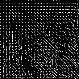
46 Optical flow Vector field function of the spatio-temporal image brightness variations Picture courtesy of Selim Temizer - Learning and Intelligent Systems (LIS) Group, MIT

47 Optical Flow Pierre Kornprobst's Demo


48 Optical Flow Examples Translation Rotation Traslation + Scaling

49 Aperture Problem In degenerate local regions, only the normal velocity is measurable.
50 The aperture problem 12/12/ :44 58

51 Optical Flow as Seen from an Aircraft Arrows show the optic flow Blue circle directly at the center shows the "focus of expansion, which tells the aircraft the specific direction it is flying. 59
52 Optical Flow: Iterative Refinement Estimate velocity at each pixel using one iteration of Lucas and Kanade estimation. Refine estimate by repeating the process estimate update Initial guess: Estimate: x 0 x 67
53 Optical Flow: Iterative Estimation estimate update Initial guess: Estimate: x 0 x 68
54 Optical Flow: Iterative Estimation estimate update Initial guess: Estimate: x 0 x 69
55 Optical Flow: Iterative Estimation x 0 x 70
56 Optical Flow: Aliasing Temporal aliasing causes ambiguities in optical flow because images can have many pixels with the same intensity. I.e., how do we know which correspondence is correct? actual shift estimated shift nearest match is correct (no aliasing) nearest match is incorrect (aliasing) To overcome aliasing: coarse-to-fine estimation. 71
57 Computing Optical Flow: Improvements Larger motion: how to maintain differential approximation? Solution: iterate Even better: adjust window / smoothing Early iterations: use larger Gaussians to allow more motion Late iterations: use less blur to find exact solution, lock on to highfrequency detail

 How")
58 Revisiting the Small Motion Assumption Is this motion small enough? Probably not it s much larger than few pixels (2 nd order terms dominate) How might we solve this problem?
59

60 SSD Surface -- Edge 75


61 SSD Surface Textured area 76
62 SSD homogeneous area 77
63 Reduce the Resolution!
64 Coarse-to-fine Optical Flow Estimation u=1.25 pixels u=2.5 pixels u=5 pixels image H u=10 pixels image I Gaussian pyramid of image H Gaussian pyramid of image I
65 Coarse-to-fine Optical Flow Estimation run iterative OF upsample run iterative OF... image HJ image I I Gaussian pyramid of image H Gaussian pyramid of image I
66 Coarse-to-fine estimation J pyramid construction V in J warp J w refine I + V J warp J w refine I + DV DV I pyramid construction J warp J w refine I + DV V out
67 Optical Flow Assumptions: 82 * Slide from Michael Black, CS

68 Optical Flow Assumptions: 83 * Slide from Michael Black, CS
69 Regularization Horn and Schunk (1981) Add global smoothness term Smoothness error: Error in brightness constancy equation E E D u u v v dxdy s x y x 2 I u I v I dx dy c x y D t y Minimize: E c E s Solve by calculus of variations
70 Deployment of Video segmentation Segment the video into multiple coherently moving objects Background subtraction Boundary detection Motion segmentation
71 Layered Representation For scenes with multiple affine motions, for each one: Estimate dominant motion parameters Reject pixels which do not fit Convergence Restart on remaining pixels


72 Layered motion Break image sequence up into layers : = Describe each layer s motion For each layer: stabilize the sequence with the affine motion compute median value at each pixel Determine occlusion relationships J. Y. A. Wang and E. H. Adelson. Representing moving images with layers. IEEE Transactions on Image Processing, 3(5): , September

73 Image Data Sets Poor resolution Amount of occlusion Low contrast Velocities ~2 p/f Primarily dilational Velocities <1 pixel/ frame The cube is rotating counterclockwise on a turntable Velocities on the table 1.2~1.4 p/f Velocities on the cube 0.2~0.5 p/f Four moving objects Speeds Taxi 1.0 p/f Car 3.0 p/f Van 3.0 p/f Pedestrian 0.3 p/f
74 Results: Horn-Schunck
75 Results: Lucas-Kanade
76 Other break-downs Brightness constancy is not satisfied Correlation based methods A point does not move like its neighbors what is the ideal window size? Regularization based methods The motion is not small (Taylor expansion doesn t hold) Use multi-scale estimation The screen is stationary yet displays motion Homogeneous objects generate zero optical flow. Fixed sphere. Changing light source. Degenerated local regions Non-rigid texture motion
77 Optical Snow Optical snow is the type of motion an observer sees when watching a snow fall. Flakes that are closer to the observer appear to move faster than flakes which are farther away.

78 Optical Flow: Where do pixels move to?
Spatial track: motion modeling
 Spatial track: motion modeling Virginio Cantoni Computer Vision and Multimedia Lab Università di Pavia Via A. Ferrata 1, 27100 Pavia virginio.cantoni@unipv.it http://vision.unipv.it/va 1 Comparison between
Peripheral drift illusion
 Peripheral drift illusion Does it work on other animals? Computer Vision Motion and Optical Flow Many slides adapted from J. Hays, S. Seitz, R. Szeliski, M. Pollefeys, K. Grauman and others Video A video
CS 4495 Computer Vision Motion and Optic Flow
 CS 4495 Computer Vision Aaron Bobick School of Interactive Computing Administrivia PS4 is out, due Sunday Oct 27 th. All relevant lectures posted Details about Problem Set: You may *not* use built in Harris
Feature Tracking and Optical Flow
 Feature Tracking and Optical Flow Prof. D. Stricker Doz. G. Bleser Many slides adapted from James Hays, Derek Hoeim, Lana Lazebnik, Silvio Saverse, who 1 in turn adapted slides from Steve Seitz, Rick Szeliski,
Feature Tracking and Optical Flow
 Feature Tracking and Optical Flow Prof. D. Stricker Doz. G. Bleser Many slides adapted from James Hays, Derek Hoeim, Lana Lazebnik, Silvio Saverse, who in turn adapted slides from Steve Seitz, Rick Szeliski,
Computer Vision Lecture 20
 Computer Perceptual Vision and Sensory WS 16/17 Augmented Computing Computer Perceptual Vision and Sensory WS 16/17 Augmented Computing Computer Perceptual Vision and Sensory WS 16/17 Augmented Computing
Computer Vision Lecture 20
 Computer Perceptual Vision and Sensory WS 16/76 Augmented Computing Many slides adapted from K. Grauman, S. Seitz, R. Szeliski, M. Pollefeys, S. Lazebnik Computer Vision Lecture 20 Motion and Optical Flow
Multi-stable Perception. Necker Cube
 Multi-stable Perception Necker Cube Spinning dancer illusion, Nobuyuki Kayahara Multiple view geometry Stereo vision Epipolar geometry Lowe Hartley and Zisserman Depth map extraction Essential matrix
Finally: Motion and tracking. Motion 4/20/2011. CS 376 Lecture 24 Motion 1. Video. Uses of motion. Motion parallax. Motion field
 Finally: Motion and tracking Tracking objects, video analysis, low level motion Motion Wed, April 20 Kristen Grauman UT-Austin Many slides adapted from S. Seitz, R. Szeliski, M. Pollefeys, and S. Lazebnik
Comparison between Motion Analysis and Stereo
 MOTION ESTIMATION The slides are from several sources through James Hays (Brown); Silvio Savarese (U. of Michigan); Octavia Camps (Northeastern); including their own slides. Comparison between Motion Analysis
Dense Image-based Motion Estimation Algorithms & Optical Flow
 Dense mage-based Motion Estimation Algorithms & Optical Flow Video A video is a sequence of frames captured at different times The video data is a function of v time (t) v space (x,y) ntroduction to motion
EE795: Computer Vision and Intelligent Systems
 EE795: Computer Vision and Intelligent Systems Spring 2012 TTh 17:30-18:45 FDH 204 Lecture 14 130307 http://www.ee.unlv.edu/~b1morris/ecg795/ 2 Outline Review Stereo Dense Motion Estimation Translational
Motion and Optical Flow. Slides from Ce Liu, Steve Seitz, Larry Zitnick, Ali Farhadi
 Motion and Optical Flow Slides from Ce Liu, Steve Seitz, Larry Zitnick, Ali Farhadi We live in a moving world Perceiving, understanding and predicting motion is an important part of our daily lives Motion
Visual motion. Many slides adapted from S. Seitz, R. Szeliski, M. Pollefeys
 Visual motion Man slides adapted from S. Seitz, R. Szeliski, M. Pollefes Motion and perceptual organization Sometimes, motion is the onl cue Motion and perceptual organization Sometimes, motion is the
VC 11/12 T11 Optical Flow
 VC 11/12 T11 Optical Flow Mestrado em Ciência de Computadores Mestrado Integrado em Engenharia de Redes e Sistemas Informáticos Miguel Tavares Coimbra Outline Optical Flow Constraint Equation Aperture
Computer Vision Lecture 20
 Computer Vision Lecture 2 Motion and Optical Flow Bastian Leibe RWTH Aachen http://www.vision.rwth-aachen.de leibe@vision.rwth-aachen.de 28.1.216 Man slides adapted from K. Grauman, S. Seitz, R. Szeliski,
CS6670: Computer Vision
 CS6670: Computer Vision Noah Snavely Lecture 19: Optical flow http://en.wikipedia.org/wiki/barberpole_illusion Readings Szeliski, Chapter 8.4-8.5 Announcements Project 2b due Tuesday, Nov 2 Please sign
Lecture 19: Motion. Effect of window size 11/20/2007. Sources of error in correspondences. Review Problem set 3. Tuesday, Nov 20
 Lecture 19: Motion Review Problem set 3 Dense stereo matching Sparse stereo matching Indexing scenes Tuesda, Nov 0 Effect of window size W = 3 W = 0 Want window large enough to have sufficient intensit
Lecture 16: Computer Vision
 CS4442/9542b: Artificial Intelligence II Prof. Olga Veksler Lecture 16: Computer Vision Motion Slides are from Steve Seitz (UW), David Jacobs (UMD) Outline Motion Estimation Motion Field Optical Flow Field
Lecture 16: Computer Vision
 CS442/542b: Artificial ntelligence Prof. Olga Veksler Lecture 16: Computer Vision Motion Slides are from Steve Seitz (UW), David Jacobs (UMD) Outline Motion Estimation Motion Field Optical Flow Field Methods
EE795: Computer Vision and Intelligent Systems
 EE795: Computer Vision and Intelligent Systems Spring 2012 TTh 17:30-18:45 FDH 204 Lecture 11 140311 http://www.ee.unlv.edu/~b1morris/ecg795/ 2 Outline Motion Analysis Motivation Differential Motion Optical
COMPUTER VISION > OPTICAL FLOW UTRECHT UNIVERSITY RONALD POPPE
 COMPUTER VISION 2017-2018 > OPTICAL FLOW UTRECHT UNIVERSITY RONALD POPPE OUTLINE Optical flow Lucas-Kanade Horn-Schunck Applications of optical flow Optical flow tracking Histograms of oriented flow Assignment
Ninio, J. and Stevens, K. A. (2000) Variations on the Hermann grid: an extinction illusion. Perception, 29,
 Variations on the Hermann grid: an extinction illusion. Perception, 29,") Ninio, J. and Stevens, K. A. (2000) Variations on the Hermann grid: an extinction illusion. Perception, 29, 1209-1217. CS 4495 Computer Vision A. Bobick Sparse to Dense Correspodence Building Rome in
Ninio, J. and Stevens, K. A. (2000) Variations on the Hermann grid: an extinction illusion. Perception, 29, 1209-1217. CS 4495 Computer Vision A. Bobick Sparse to Dense Correspodence Building Rome in
Optical flow and tracking
 EECS 442 Computer vision Optical flow and tracking Intro Optical flow and feature tracking Lucas-Kanade algorithm Motion segmentation Segments of this lectures are courtesy of Profs S. Lazebnik S. Seitz,
Visual Tracking. Image Processing Laboratory Dipartimento di Matematica e Informatica Università degli studi di Catania.
 Image Processing Laboratory Dipartimento di Matematica e Informatica Università degli studi di Catania 1 What is visual tracking? estimation of the target location over time 2 applications Six main areas:
Motion. 1 Introduction. 2 Optical Flow. Sohaib A Khan. 2.1 Brightness Constancy Equation
 Motion Sohaib A Khan 1 Introduction So far, we have dealing with single images of a static scene taken by a fixed camera. Here we will deal with sequence of images taken at different time intervals. Motion
Visual Tracking. Antonino Furnari. Image Processing Lab Dipartimento di Matematica e Informatica Università degli Studi di Catania
 Visual Tracking Antonino Furnari Image Processing Lab Dipartimento di Matematica e Informatica Università degli Studi di Catania furnari@dmi.unict.it 11 giugno 2015 What is visual tracking? estimation
EE 264: Image Processing and Reconstruction. Image Motion Estimation I. EE 264: Image Processing and Reconstruction. Outline
 1 Image Motion Estimation I 2 Outline 1. Introduction to Motion 2. Why Estimate Motion? 3. Global vs. Local Motion 4. Block Motion Estimation 5. Optical Flow Estimation Basics 6. Optical Flow Estimation
Motion and Tracking. Andrea Torsello DAIS Università Ca Foscari via Torino 155, Mestre (VE)
") Motion and Tracking Andrea Torsello DAIS Università Ca Foscari via Torino 155, 30172 Mestre (VE) Motion Segmentation Segment the video into multiple coherently moving objects Motion and Perceptual Organization
Motion and Tracking Andrea Torsello DAIS Università Ca Foscari via Torino 155, 30172 Mestre (VE) Motion Segmentation Segment the video into multiple coherently moving objects Motion and Perceptual Organization
Fundamental matrix. Let p be a point in left image, p in right image. Epipolar relation. Epipolar mapping described by a 3x3 matrix F
 Fundamental matrix Let p be a point in left image, p in right image l l Epipolar relation p maps to epipolar line l p maps to epipolar line l p p Epipolar mapping described by a 3x3 matrix F Fundamental
Range Imaging Through Triangulation. Range Imaging Through Triangulation. Range Imaging Through Triangulation. Range Imaging Through Triangulation
 Obviously, this is a very slow process and not suitable for dynamic scenes. To speed things up, we can use a laser that projects a vertical line of light onto the scene. This laser rotates around its vertical
Ruch (Motion) Rozpoznawanie Obrazów Krzysztof Krawiec Instytut Informatyki, Politechnika Poznańska. Krzysztof Krawiec IDSS
 Rozpoznawanie Obrazów Krzysztof Krawiec Instytut Informatyki, Politechnika Poznańska. Krzysztof Krawiec IDSS") Ruch (Motion) Rozpoznawanie Obrazów Krzysztof Krawiec Instytut Informatyki, Politechnika Poznańska 1 Krzysztof Krawiec IDSS 2 The importance of visual motion Adds entirely new (temporal) dimension to visual
Ruch (Motion) Rozpoznawanie Obrazów Krzysztof Krawiec Instytut Informatyki, Politechnika Poznańska 1 Krzysztof Krawiec IDSS 2 The importance of visual motion Adds entirely new (temporal) dimension to visual
Motion Estimation. There are three main types (or applications) of motion estimation:
 of motion estimation:") Members: D91922016 朱威達 R93922010 林聖凱 R93922044 謝俊瑋 Motion Estimation There are three main types (or applications) of motion estimation: Parametric motion (image alignment) The main idea of parametric motion
Members: D91922016 朱威達 R93922010 林聖凱 R93922044 謝俊瑋 Motion Estimation There are three main types (or applications) of motion estimation: Parametric motion (image alignment) The main idea of parametric motion
EECS 556 Image Processing W 09
 EECS 556 Image Processing W 09 Motion estimation Global vs. Local Motion Block Motion Estimation Optical Flow Estimation (normal equation) Man slides of this lecture are courtes of prof Milanfar (UCSC)
Optic Flow and Basics Towards Horn-Schunck 1
 Optic Flow and Basics Towards Horn-Schunck 1 Lecture 7 See Section 4.1 and Beginning of 4.2 in Reinhard Klette: Concise Computer Vision Springer-Verlag, London, 2014 1 See last slide for copyright information.
Visual Tracking (1) Tracking of Feature Points and Planar Rigid Objects
 Tracking of Feature Points and Planar Rigid Objects") Intelligent Control Systems Visual Tracking (1) Tracking of Feature Points and Planar Rigid Objects Shingo Kagami Graduate School of Information Sciences, Tohoku University swk(at)ic.is.tohoku.ac.jp http://www.ic.is.tohoku.ac.jp/ja/swk/
Intelligent Control Systems Visual Tracking (1) Tracking of Feature Points and Planar Rigid Objects Shingo Kagami Graduate School of Information Sciences, Tohoku University swk(at)ic.is.tohoku.ac.jp http://www.ic.is.tohoku.ac.jp/ja/swk/
ECE Digital Image Processing and Introduction to Computer Vision
 ECE592-064 Digital Image Processing and Introduction to Computer Vision Depart. of ECE, NC State University Instructor: Tianfu (Matt) Wu Spring 2017 Recap, SIFT Motion Tracking Change Detection Feature
Motion Analysis. Motion analysis. Now we will talk about. Differential Motion Analysis. Motion analysis. Difference Pictures
 Now we will talk about Motion Analysis Motion analysis Motion analysis is dealing with three main groups of motionrelated problems: Motion detection Moving object detection and location. Derivation of
Automatic Image Alignment (direct) with a lot of slides stolen from Steve Seitz and Rick Szeliski
 with a lot of slides stolen from Steve Seitz and Rick Szeliski") Automatic Image Alignment (direct) with a lot of slides stolen from Steve Seitz and Rick Szeliski 15-463: Computational Photography Alexei Efros, CMU, Fall 2005 Today Go over Midterm Go over Project #3
Automatic Image Alignment (direct) with a lot of slides stolen from Steve Seitz and Rick Szeliski 15-463: Computational Photography Alexei Efros, CMU, Fall 2005 Today Go over Midterm Go over Project #3
Optical Flow CS 637. Fuxin Li. With materials from Kristen Grauman, Richard Szeliski, S. Narasimhan, Deqing Sun
 Optical Flow CS 637 Fuxin Li With materials from Kristen Grauman, Richard Szeliski, S. Narasimhan, Deqing Sun Motion and perceptual organization Sometimes, motion is the only cue Motion and perceptual
Matching. Compare region of image to region of image. Today, simplest kind of matching. Intensities similar.
 Matching Compare region of image to region of image. We talked about this for stereo. Important for motion. Epipolar constraint unknown. But motion small. Recognition Find object in image. Recognize object.
Lucas-Kanade Motion Estimation. Thanks to Steve Seitz, Simon Baker, Takeo Kanade, and anyone else who helped develop these slides.
 Lucas-Kanade Motion Estimation Thanks to Steve Seitz, Simon Baker, Takeo Kanade, and anyone else who helped develop these slides. 1 Why estimate motion? We live in a 4-D world Wide applications Object
Optical Flow-Based Motion Estimation. Thanks to Steve Seitz, Simon Baker, Takeo Kanade, and anyone else who helped develop these slides.
 Optical Flow-Based Motion Estimation Thanks to Steve Seitz, Simon Baker, Takeo Kanade, and anyone else who helped develop these slides. 1 Why estimate motion? We live in a 4-D world Wide applications Object
CS 4495 Computer Vision A. Bobick. Motion and Optic Flow. Stereo Matching
 Stereo Matching Fundamental matrix Let p be a point in left image, p in right image l l Epipolar relation p maps to epipolar line l p maps to epipolar line l p p Epipolar mapping described by a 3x3 matrix
Mariya Zhariy. Uttendorf Introduction to Optical Flow. Mariya Zhariy. Introduction. Determining. Optical Flow. Results. Motivation Definition
 to Constraint to Uttendorf 2005 Contents to Constraint 1 Contents to Constraint 1 2 Constraint Contents to Constraint 1 2 Constraint 3 Visual cranial reflex(vcr)(?) to Constraint Rapidly changing scene
Overview. Video. Overview 4/7/2008. Optical flow. Why estimate motion? Motion estimation: Optical flow. Motion Magnification Colorization.
 Overview Video Optical flow Motion Magnification Colorization Lecture 9 Optical flow Motion Magnification Colorization Overview Optical flow Combination of slides from Rick Szeliski, Steve Seitz, Alyosha
Lecture 20: Tracking. Tuesday, Nov 27
 Lecture 20: Tracking Tuesday, Nov 27 Paper reviews Thorough summary in your own words Main contribution Strengths? Weaknesses? How convincing are the experiments? Suggestions to improve them? Extensions?
CS 565 Computer Vision. Nazar Khan PUCIT Lectures 15 and 16: Optic Flow
 CS 565 Computer Vision Nazar Khan PUCIT Lectures 15 and 16: Optic Flow Introduction Basic Problem given: image sequence f(x, y, z), where (x, y) specifies the location and z denotes time wanted: displacement
EXAM SOLUTIONS. Image Processing and Computer Vision Course 2D1421 Monday, 13 th of March 2006,
 School of Computer Science and Communication, KTH Danica Kragic EXAM SOLUTIONS Image Processing and Computer Vision Course 2D1421 Monday, 13 th of March 2006, 14.00 19.00 Grade table 0-25 U 26-35 3 36-45
Announcements. Computer Vision I. Motion Field Equation. Revisiting the small motion assumption. Visual Tracking. CSE252A Lecture 19.
 Visual Tracking CSE252A Lecture 19 Hw 4 assigned Announcements No class on Thursday 12/6 Extra class on Tuesday 12/4 at 6:30PM in WLH Room 2112 Motion Field Equation Measurements I x = I x, T: Components
CPSC 425: Computer Vision
 1 / 49 CPSC 425: Computer Vision Instructor: Fred Tung ftung@cs.ubc.ca Department of Computer Science University of British Columbia Lecture Notes 2015/2016 Term 2 2 / 49 Menu March 10, 2016 Topics: Motion
Notes 9: Optical Flow
 Course 049064: Variational Methods in Image Processing Notes 9: Optical Flow Guy Gilboa 1 Basic Model 1.1 Background Optical flow is a fundamental problem in computer vision. The general goal is to find
Motion. CS 554 Computer Vision Pinar Duygulu Bilkent University
 1 Motion CS 554 Computer Vision Pinar Duygulu Bilkent University 2 Motion A lot of information can be extracted from time varying sequences of images, often more easily than from static images. e.g, camouflaged
ELEC Dr Reji Mathew Electrical Engineering UNSW
 ELEC 4622 Dr Reji Mathew Electrical Engineering UNSW Review of Motion Modelling and Estimation Introduction to Motion Modelling & Estimation Forward Motion Backward Motion Block Motion Estimation Motion
Visual Tracking (1) Feature Point Tracking and Block Matching
 Feature Point Tracking and Block Matching") Intelligent Control Systems Visual Tracking (1) Feature Point Tracking and Block Matching Shingo Kagami Graduate School of Information Sciences, Tohoku University swk(at)ic.is.tohoku.ac.jp http://www.ic.is.tohoku.ac.jp/ja/swk/
Intelligent Control Systems Visual Tracking (1) Feature Point Tracking and Block Matching Shingo Kagami Graduate School of Information Sciences, Tohoku University swk(at)ic.is.tohoku.ac.jp http://www.ic.is.tohoku.ac.jp/ja/swk/
Capturing, Modeling, Rendering 3D Structures
 Computer Vision Approach Capturing, Modeling, Rendering 3D Structures Calculate pixel correspondences and extract geometry Not robust Difficult to acquire illumination effects, e.g. specular highlights
CS201: Computer Vision Introduction to Tracking
 CS201: Computer Vision Introduction to Tracking John Magee 18 November 2014 Slides courtesy of: Diane H. Theriault Question of the Day How can we represent and use motion in images? 1 What is Motion? Change
Practice Exam Sample Solutions
 CS 675 Computer Vision Instructor: Marc Pomplun Practice Exam Sample Solutions Note that in the actual exam, no calculators, no books, and no notes allowed. Question 1: out of points Question 2: out of
CHAPTER 5 MOTION DETECTION AND ANALYSIS
 CHAPTER 5 MOTION DETECTION AND ANALYSIS 5.1. Introduction: Motion processing is gaining an intense attention from the researchers with the progress in motion studies and processing competence. A series
SURVEY OF LOCAL AND GLOBAL OPTICAL FLOW WITH COARSE TO FINE METHOD
 SURVEY OF LOCAL AND GLOBAL OPTICAL FLOW WITH COARSE TO FINE METHOD M.E-II, Department of Computer Engineering, PICT, Pune ABSTRACT: Optical flow as an image processing technique finds its applications
1 (5 max) 2 (10 max) 3 (20 max) 4 (30 max) 5 (10 max) 6 (15 extra max) total (75 max + 15 extra)
 2 (10 max) 3 (20 max) 4 (30 max) 5 (10 max) 6 (15 extra max) total (75 max + 15 extra)") Mierm Exam CS223b Stanford CS223b Computer Vision, Winter 2004 Feb. 18, 2004 Full Name: Email: This exam has 7 pages. Make sure your exam is not missing any sheets, and write your name on every page. The
Mierm Exam CS223b Stanford CS223b Computer Vision, Winter 2004 Feb. 18, 2004 Full Name: Email: This exam has 7 pages. Make sure your exam is not missing any sheets, and write your name on every page. The
BSB663 Image Processing Pinar Duygulu. Slides are adapted from Selim Aksoy
 BSB663 Image Processing Pinar Duygulu Slides are adapted from Selim Aksoy Image matching Image matching is a fundamental aspect of many problems in computer vision. Object or scene recognition Solving
Leow Wee Kheng CS4243 Computer Vision and Pattern Recognition. Motion Tracking. CS4243 Motion Tracking 1
 Leow Wee Kheng CS4243 Computer Vision and Pattern Recognition Motion Tracking CS4243 Motion Tracking 1 Changes are everywhere! CS4243 Motion Tracking 2 Illumination change CS4243 Motion Tracking 3 Shape
Chapter 3 Image Registration. Chapter 3 Image Registration
 Chapter 3 Image Registration Distributed Algorithms for Introduction (1) Definition: Image Registration Input: 2 images of the same scene but taken from different perspectives Goal: Identify transformation
Computer Vision for HCI. Motion. Motion
 Computer Vision for HCI Motion Motion Changing scene may be observed in a sequence of images Changing pixels in image sequence provide important features for object detection and activity recognition 2
Stereo Vision. MAN-522 Computer Vision
 Stereo Vision MAN-522 Computer Vision What is the goal of stereo vision? The recovery of the 3D structure of a scene using two or more images of the 3D scene, each acquired from a different viewpoint in
CS 4495 Computer Vision A. Bobick. Motion and Optic Flow. Stereo Matching
 Stereo Matching Fundamental matrix Let p be a point in left image, p in right image l l Epipolar relation p maps to epipolar line l p maps to epipolar line l p p Epipolar mapping described by a 3x3 matrix
Introduction to Computer Vision
 Introduction to Computer Vision Michael J. Black Nov 2009 Perspective projection and affine motion Goals Today Perspective projection 3D motion Wed Projects Friday Regularization and robust statistics
Announcements. Motion. Structure-from-Motion (SFM) Motion. Discrete Motion: Some Counting
 Motion. Discrete Motion: Some Counting") Announcements Motion Introduction to Computer Vision CSE 152 Lecture 20 HW 4 due Friday at Midnight Final Exam: Tuesday, 6/12 at 8:00AM-11:00AM, regular classroom Extra Office Hours: Monday 6/11 9:00AM-10:00AM
Announcements Motion Introduction to Computer Vision CSE 152 Lecture 20 HW 4 due Friday at Midnight Final Exam: Tuesday, 6/12 at 8:00AM-11:00AM, regular classroom Extra Office Hours: Monday 6/11 9:00AM-10:00AM
Robert Collins CSE598G. Intro to Template Matching and the Lucas-Kanade Method
 Intro to Template Matching and the Lucas-Kanade Method Appearance-Based Tracking current frame + previous location likelihood over object location current location appearance model (e.g. image template,
Local Feature Detectors
 Local Feature Detectors Selim Aksoy Department of Computer Engineering Bilkent University saksoy@cs.bilkent.edu.tr Slides adapted from Cordelia Schmid and David Lowe, CVPR 2003 Tutorial, Matthew Brown,
Final Exam Study Guide
 Final Exam Study Guide Exam Window: 28th April, 12:00am EST to 30th April, 11:59pm EST Description As indicated in class the goal of the exam is to encourage you to review the material from the course.
CS-465 Computer Vision
 CS-465 Computer Vision Nazar Khan PUCIT 9. Optic Flow Optic Flow Nazar Khan Computer Vision 2 / 25 Optic Flow Nazar Khan Computer Vision 3 / 25 Optic Flow Where does pixel (x, y) in frame z move to in
Outline 7/2/201011/6/
 Outline Pattern recognition in computer vision Background on the development of SIFT SIFT algorithm and some of its variations Computational considerations (SURF) Potential improvement Summary 01 2 Pattern
Optic Flow and Motion Detection
 Optic Flow and Motion Detection Computer Vision and Imaging Martin Jagersand Readings: Szeliski Ch 8 Ma, Kosecka, Sastry Ch 4 Image motion Somehow quantify the frame-to to-frame differences in image sequences.
Segmentation and Tracking of Partial Planar Templates
 Segmentation and Tracking of Partial Planar Templates Abdelsalam Masoud William Hoff Colorado School of Mines Colorado School of Mines Golden, CO 800 Golden, CO 800 amasoud@mines.edu whoff@mines.edu Abstract
C18 Computer vision. C18 Computer Vision. This time... Introduction. Outline.
 C18 Computer Vision. This time... 1. Introduction; imaging geometry; camera calibration. 2. Salient feature detection edges, line and corners. 3. Recovering 3D from two images I: epipolar geometry. C18
Image processing and features
 Image processing and features Gabriele Bleser gabriele.bleser@dfki.de Thanks to Harald Wuest, Folker Wientapper and Marc Pollefeys Introduction Previous lectures: geometry Pose estimation Epipolar geometry
CS231A Section 6: Problem Set 3
 CS231A Section 6: Problem Set 3 Kevin Wong Review 6 -! 1 11/09/2012 Announcements PS3 Due 2:15pm Tuesday, Nov 13 Extra Office Hours: Friday 6 8pm Huang Common Area, Basement Level. Review 6 -! 2 Topics
Marcel Worring Intelligent Sensory Information Systems
 Marcel Worring worring@science.uva.nl Intelligent Sensory Information Systems University of Amsterdam Information and Communication Technology archives of documentaries, film, or training material, video
CS664 Lecture #18: Motion
 CS664 Lecture #18: Motion Announcements Most paper choices were fine Please be sure to email me for approval, if you haven t already This is intended to help you, especially with the final project Use
The 2D/3D Differential Optical Flow
 The 2D/3D Differential Optical Flow Prof. John Barron Dept. of Computer Science University of Western Ontario London, Ontario, Canada, N6A 5B7 Email: barron@csd.uwo.ca Phone: 519-661-2111 x86896 Canadian
Final Exam Study Guide CSE/EE 486 Fall 2007
 Final Exam Study Guide CSE/EE 486 Fall 2007 Lecture 2 Intensity Sufaces and Gradients Image visualized as surface. Terrain concepts. Gradient of functions in 1D and 2D Numerical derivatives. Taylor series.
Chapter 9 Object Tracking an Overview
 Chapter 9 Object Tracking an Overview The output of the background subtraction algorithm, described in the previous chapter, is a classification (segmentation) of pixels into foreground pixels (those belonging
Stereo. 11/02/2012 CS129, Brown James Hays. Slides by Kristen Grauman
 Stereo 11/02/2012 CS129, Brown James Hays Slides by Kristen Grauman Multiple views Multi-view geometry, matching, invariant features, stereo vision Lowe Hartley and Zisserman Why multiple views? Structure
SUMMARY: DISTINCTIVE IMAGE FEATURES FROM SCALE- INVARIANT KEYPOINTS
 SUMMARY: DISTINCTIVE IMAGE FEATURES FROM SCALE- INVARIANT KEYPOINTS Cognitive Robotics Original: David G. Lowe, 004 Summary: Coen van Leeuwen, s1460919 Abstract: This article presents a method to extract
Optical Flow Estimation
 Optical Flow Estimation Goal: Introduction to image motion and 2D optical flow estimation. Motivation: Motion is a rich source of information about the world: segmentation surface structure from parallax
Representing Moving Images with Layers. J. Y. Wang and E. H. Adelson MIT Media Lab
 Representing Moving Images with Layers J. Y. Wang and E. H. Adelson MIT Media Lab Goal Represent moving images with sets of overlapping layers Layers are ordered in depth and occlude each other Velocity
Augmented Reality VU. Computer Vision 3D Registration (2) Prof. Vincent Lepetit
 Prof. Vincent Lepetit") Augmented Reality VU Computer Vision 3D Registration (2) Prof. Vincent Lepetit Feature Point-Based 3D Tracking Feature Points for 3D Tracking Much less ambiguous than edges; Point-to-point reprojection
Augmented Reality VU Computer Vision 3D Registration (2) Prof. Vincent Lepetit Feature Point-Based 3D Tracking Feature Points for 3D Tracking Much less ambiguous than edges; Point-to-point reprojection
Optical Flow Estimation with CUDA. Mikhail Smirnov
 Optical Flow Estimation with CUDA Mikhail Smirnov msmirnov@nvidia.com Document Change History Version Date Responsible Reason for Change Mikhail Smirnov Initial release Abstract Optical flow is the apparent
Computer Vision Lecture 18
 Course Outline Computer Vision Lecture 8 Motion and Optical Flow.0.009 Bastian Leibe RWTH Aachen http://www.umic.rwth-aachen.de/multimedia leibe@umic.rwth-aachen.de Man slides adapted from K. Grauman,
Hand-Eye Calibration from Image Derivatives
 Hand-Eye Calibration from Image Derivatives Abstract In this paper it is shown how to perform hand-eye calibration using only the normal flow field and knowledge about the motion of the hand. The proposed
Correspondence and Stereopsis. Original notes by W. Correa. Figures from [Forsyth & Ponce] and [Trucco & Verri]
![Correspondence and Stereopsis. Original notes by W. Correa. Figures from [Forsyth & Ponce] and [Trucco & Verri]](/thumbs/80/81283374.jpg "Correspondence and Stereopsis. Original notes by W. Correa. Figures from [Forsyth & Ponce] and [Trucco & Verri]") Correspondence and Stereopsis Original notes by W. Correa. Figures from [Forsyth & Ponce] and [Trucco & Verri] Introduction Disparity: Informally: difference between two pictures Allows us to gain a strong
Correspondence and Stereopsis Original notes by W. Correa. Figures from [Forsyth & Ponce] and [Trucco & Verri] Introduction Disparity: Informally: difference between two pictures Allows us to gain a strong
Complex Sensors: Cameras, Visual Sensing. The Robotics Primer (Ch. 9) ECE 497: Introduction to Mobile Robotics -Visual Sensors
 ECE 497: Introduction to Mobile Robotics -Visual Sensors") Complex Sensors: Cameras, Visual Sensing The Robotics Primer (Ch. 9) Bring your laptop and robot everyday DO NOT unplug the network cables from the desktop computers or the walls Tuesday s Quiz is on Visual
Complex Sensors: Cameras, Visual Sensing The Robotics Primer (Ch. 9) Bring your laptop and robot everyday DO NOT unplug the network cables from the desktop computers or the walls Tuesday s Quiz is on Visual
Mosaics. Today s Readings
 Mosaics VR Seattle: http://www.vrseattle.com/ Full screen panoramas (cubic): http://www.panoramas.dk/ Mars: http://www.panoramas.dk/fullscreen3/f2_mars97.html Today s Readings Szeliski and Shum paper (sections
Motion detection Computing image motion Motion estimation Egomotion and structure from motion Motion classification
 Time varying image analysis Motion detection Computing image motion Motion estimation Egomotion and structure from motion Motion classification Time-varying image analysis- 1 The problems Visual surveillance
Dense 3D Reconstruction. Christiano Gava
 Dense 3D Reconstruction Christiano Gava christiano.gava@dfki.de Outline Previous lecture: structure and motion II Structure and motion loop Triangulation Today: dense 3D reconstruction The matching problem
Chaplin, Modern Times, 1936
 Chaplin, Modern Times, 1936 [A Bucket of Water and a Glass Matte: Special Effects in Modern Times; bonus feature on The Criterion Collection set] Multi-view geometry problems Structure: Given projections
Optical flow. Cordelia Schmid
 Optical flow Cordelia Schmid Motion field The motion field is the projection of the 3D scene motion into the image Optical flow Definition: optical flow is the apparent motion of brightness patterns in
Minimizing Noise and Bias in 3D DIC. Correlated Solutions, Inc.
 Minimizing Noise and Bias in 3D DIC Correlated Solutions, Inc. Overview Overview of Noise and Bias Digital Image Correlation Background/Tracking Function Minimizing Noise Focus Contrast/Lighting Glare