Visual Tracking. Image Processing Laboratory Dipartimento di Matematica e Informatica Università degli studi di Catania.

Transcription

1 Image Processing Laboratory Dipartimento di Matematica e Informatica Università degli studi di Catania 1

2 What is visual tracking? estimation of the target location over time 2

3 applications Six main areas: 3 Media production and augmented reality Medical applications and biological research Surveillance and business applications Robotics and unmanned vehicles Tele-collaboration and interactive gaming Art installations and performances

4 Applications motion capture: videogames, movies 4

5 Applications performance analysis: sport 5

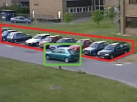
6 Applications video surveillance 6

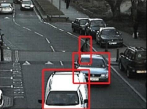
7 Applications traffic monitoring 7

8 Problem Formulation estimation of the target state over time Let be the frames of a video sequence, where is the frame at time and is the space of all possible images. Tracking a single target object can be formulated as the estimation of the time series over a set of discrete time instants indexed by based on the information in. The vectors The time series are the states of the target and is also known as the trajectory of the target in The information encoded in the state 8 is the state space. depend on the application..

9 Problem Formulation object state 9

10 Problem Formulation feature extraction estimation of the target state over time may be mapped onto a feature (or observation) space that highlights information relevant to the tracking problem. The observation generated by a target is encoded in. The operations that are necessary to transform the image space observation space to the are referred to as feature extraction. Visual trackers propagate the information in the state over time using the extracted features. A localization strategy defines how to use the image features to produce an estimate of the target state 10.

11 Problem Formulation feature extraction 11 : space of all possible images : state space : feature or observation space : time index

12 Challenges 12

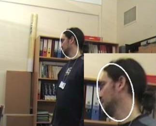
13 Challenges occlusion - clutter 13

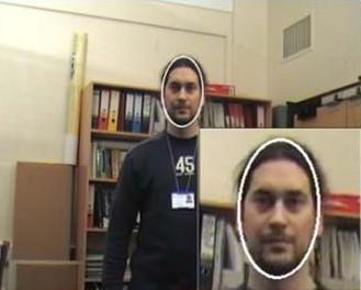
14 Challenges change of appearance 14

15 Pipeline : video frames 15 : observations : object states

16 Techniques Visual tracking techniques can be characterized by the way the object is represented and the way the object is located Techniques Template Based Tracking NCC (Rigid) 16 Lucas-Kanade affine tracker Local Feature Based Tracking Lucas-Kanade optical flow Region Based Tracking CAMSHIFT Kernel Based

17 Template Based Tracking Objects are represented as image patches and located by maximizing some similarity measure between the template object and a series of candidates extracted from the current frame (template matching). target object where «w,h» are the template dimensions and «x,y» is the considered sub-image position within the frame. 17

18 Similarity Measures In order to measure the similarity degree between the target object and the candidates we need a similarity measure. Where: is the template (target object) are the template dimensions is the sub-image (candidate) is the location of the sub-image 18 Similarity measures: Sum of Absolute Differences (SAD) Sum of Squared Differences (SSD) Normalized Corss Correlation (NCC)

19 Similarity Measures sum of absolute differences (SAD) A perfect match corresponds to 0 SAD represents the norm between and. 19

20 Similarity Measures sum of squared differences (SSD) A perfect match corresponds to 0 SSD is the euclidean norm ( ) between and. 20

21 Similarity Measures normalized cross correlation (NCC) where and are the subimage and template image mean values respectively A perfect match corresponds to 1 The worst match corresponds to -1 (max decorrelation) NCC corresponds to the cosine angle between and 21

22 Similarity Measures NCC explained mean mean variance variance Fixed the point, let and vectors. The above product is: where is the be two 3d norm and product, a generalization of the dot product. For a property of the inner product, if being and are real vectors: the angle between the two vectors. only if equals multiplied by a positive scalar. i.e., invariance to linear lighting changes 22 is the inner

23 Template Matching similarity measure example Example of template matching using NCC as similarity measure The similarity function maximum position is the object location 23

24 Template Matching computational cost Number of operations = where: H and W are the dimensions of the frame. M and N are the dimensions of the template. The computational cost is proportional to the template and the frame dimensions. Possible Solutions: Multi-Resolution SubTemplate 24

25 Template Matching computational cost - improvements 1. Multi-Resolution: A low-resolution version of the template is first located in the lowest resolution image of the pyramids. This defines a search area in the next level where to search for a higher resolution template. At the last iteration the object is found in the original frame. 2. Sub-Template: First a sub-template search is performed on the entire image. Next, only on those areas with a high similarity score, a regular search is performed. 25

26 Template Matching limits Limits: The template representation is not invariant to rotation, scale and other transformations. So: The transformations have to be handled explicitly. Possible solution: Estimating the transformation parameters during the search (i.e., search for warped versions of the template). Lucas-Kanade registration algorithm 26

27 Techniques Techniques Template Based Tracking NCC (Rigid) 27 Lucas-Kanade affine tracker Local Feature Based Tracking Lucas-Kanade optical flow Region Based Tracking CAMSHIFT Kernel Based

28 Lucas-Kanade Registration Algorithm translational problem Image alignment consists of moving, and possibly deforming, a template to minimize the difference between the template and an input image. The translational image registration problem can be characterized as follows: we are given functions and which give the respective pixel values at each location in two images, where is a vector. We wish to find the disparity vector which minimizes some measure of the difference between and, for in some region of interest. estimate the 2 translation parameters 28

29 Lucas-Kanade Registration Algorithm general problem We want to search for an affine-transformed version of the template estimating the 6 parameters of the transformation matrix: estimate the 6 affine transformation parameters 29

30 Lucas-Kanade Registration Algorithm the warp function Let be the deformation function of the pixel using the vector parameters from the template coordinate system to the image one. The warp takes the pixel in the coordinate system of the template it to the sub-pixel location in the coordinate system of the image. The ( function can be a simple translation ( ). In the latter case In general the number of parameters arbitrarily complex. 30 ) or a 3D affine warp function is defined as: may be arbitrarily large and and maps can be

31 Lucas-Kanade Registration Algorithm goal The aim of the algorithm is to minimize the sum of squared errors (SSD) between the template and the image warped back onto the coordinate system of the template: (1) The minimization in (1) is performed with respect to the parameters vector sum is performed over all of the pixels of the template. and the To optimize the expression in equation (1), the Lucas-Kanade algorithm assumes that a current estimate of the vector is known and then iteratively solves for increments to the parameters ; i.e., the following expression is approximately minimized: (2) with respect to and then the parameters are updated: These two steps are iterated until the estimates of the parameters converge ( under a fixed threshold). The initial parameters estimate: is often used. is the iterative minimization process is based on the gradient descent 31

32 Lucas-Kanade Registration Algorithm derivation The equation (1) can be expressed using the Taylor series expansion stopping at the first degree: (3) where warp Jacobian: is the gradient of the image evaluated at and is the Calculating the derivative of the Taylor series expansion with respect to the parameter vector increment and equating to zero, we obtain: (4) where is the hessian defined as: (5) 32

33 Lucas-Kanade Registration Algorithm algorithm Iterate: 1 Warp with to compute 2 Compute the error image 3 Warp the gradient with 4 Evaluate the Jacobian at 5 Compute the steepest descent images 6 Compute the Hessian matrix using Equation (5) 7 Compute 8 Compute using Equation (4) 9 Update the parameters until 33 number of parameters number of pixels in Computational cost of each iteration:

34 Lucas-Kanade Registration Algorithm algorithm Input: Image Template Step 1 (image warp): warp using the current estimate of Target candidate Step 2 (error image): 34

35 Lucas-Kanade Registration Algorithm algorithm Step 3 (gradient warp): Image gradient computation image gradient warped gradient warp using the current estimate of 35

36 Lucas-Kanade Registration Algorithm algorithm Step 4 (Jacobian): It represents all the partial derivatives of the warp function with respect to the parameters vector. Step 5 (steepest descent images): warped gradient the steepest descent images act as weights 36

37 Lucas-Kanade Registration Algorithm algorithm Step 6 (Hessian matrix): which corresponds to the second derivative of the Jacobian or also to the Jacobian of the gradient of the warp function. Step 7-8 (compute ): Hessian matrix weight function Step 9 (update the parameters): iterate until 37 error image

38 Lucas Kanade Registration Algorithm pyramidal implementation In order to have better performance, a pyramidal approach can be used: First the algorithm estimate the motion vector at the highest level (less details), then the obtained values are used as starting point for the next level (more details). The height of the pyramid usually does not exceed 2-3 levels: less details more details 38

39 DEMO Template Matching 39

40 Techniques Techniques Template Based Tracking NCC (Rigid) 40 Lucas-Kanade affine tracker Local Feature Based Tracking Lucas-Kanade optical flow Region Based Tracking CAMSHIFT Kernel Based

41 Local Feature Based Tracking Objects are represented as a set of feature points (keypoints or interest points) and located by estimating the keypoints locations over time. 41

42 Local Feature Based Tracking The points are tracked independently by estimating their motion vectors at each frame. This approach is referred to as sparse optical flow 42 42

43 Optical Flow Even impoverished motion data can evoke a strong percept G. Johansson, Visual Perception of Biological Motion and a Model For Its Analysis", Perception and Psychophysics 14, ,

44 Optical Flow Even impoverished motion data can evoke a strong percept G. Johansson, Visual Perception of Biological Motion and a Model For Its Analysis", Perception and Psychophysics 14, ,

45 Optical Flow definition Optical Flow is the pattern of apparent motion of objects, surfaces and edges in a visual scene caused by the relative motion between an observer (an eye or a camera) and the scene. Two types of motion: Movement in the scene with a static camera Movement of the camera Since motion is relative anyway, these types of motion should be the same. 45 However, this is not always the case, since if the scene moves relative to the illumination, shadow effects need to be dealt with.

46 Optical Flow motion field The motion field is the projection of the 3D scene motion into the image 46

47 Optical Flow motion field 47

48 Optical Flow usages Motion flow is useful for: 48 depth map, observer motion, image segmentation, object motion: establish relationship between object & viewer, guides smooth pursuit eye movement (saccades).

49 Optical Flow motion field and pallax X(t) is a moving 3D point Velocity of scene point: V = dx/dt x(t) = (x(t), y(t)) is the projection of X in the image Apparent velocity v in the image: given by components vx = dx/dt and vy = dy/dt These components are known as the motion field of the image X(t) X(t+dt) V v x(t) x(t+dt)

50 Optical Flow aperture problem Generally, optical flow corresponds to the motion field, but not always. For example, the motion field and the optical flow of a rotating barber's pole are different. In general, such cases are unusual.

51 Optical Flow aperture problem

52 Optical Flow aperture problem Perceived motion

53 Optical Flow aperture problem Actual motion

54 Optical Flow aperture problem

55 Optical Flow aperture problem

56 Optical Flow aperture problem Each neuron in the visual system is sensitive to visual input in a small part of the visual field, as if each neuron is looking at the visual field through a small window or aperture. The motion direction of a contour is ambiguous, because the motion component parallel to the line cannot be inferred based on the visual input. This means that a variety of contours of different orientations moving at different speeds can cause identical responses in a motion sensitive neuron in the visual system.

57 Optical Flow formulation In order to track a key-point, the brightness constancy assumption is usually considered. It states that the key-points can change their position but they keep approximately the same pixel value in two subsequent frames. This means that changes in image intensity are about entirely due to motion and not to lighting changes in the scene. Given two subsequent frames respectively taken at times and in order to compute the key-point motion vector, the image constraint equation is formulated using the brightness constancy assumption: (1) Expanding the right hand side with Taylor series: (2) Using equation (1) we get: (3) 57

58 Optical Flow formulation So we get: (4) Where and are the components of the velocity of the point with coordinates,, and are the partial derivatives of with respect to, and. So we have: while (5) which is the motion constraint equation. Considering that the spatial and temporal derivatives can be computed, the Equation (5) has two unknowns ( and ) and can not be solved. So, in order to find the optical flow, additional equation have to be added. This is done by making some additional assumption. Each optical flow algorithm add its own assumption (i.e., equations). 58

59 Techniques Techniques Template Based Tracking NCC (Rigid) 59 Lucas-Kanade affine tracker Local Feature Based Tracking Lucas-Kanade optical flow Region Based Tracking CAMSHIFT Kernel Based

60 Lucas-Kanade Optical Flow assumptions Brightness Constancy: the key-points can change their position but they keep approximately the same pixel value in two subsequent frames. Spatial Coherence: neighborhood points belong to the same surface and so they share the same velocity Temporal Persistence: the movements of an object in the scene are very slow. This means that the temporal increments are faster than object movements assumption 2 allows us to apply the L-K algorithm to an image patch surrounding the key-point 60

61 Lucas-Kanade Optical Flow formulation The motion constraint equation (5) can be written as: (6) where Given the key-point, a window containing neighbor pixels and the following equations are obtained from (6): is considered We can write the system as: (7) 61

62 Lucas-Kanade Optical Flow formulation where: The equation (7) represents an over-determined system which can be solved with the least squares as follows: The optical flow (i.e., the motion vector) is finally computed as: structure tensor 62

63 Lucas-Kanade Optical Flow good features to track Not all parts of an image contain motion information. Similarly, along a straight edge, we can only determine the motion component orthogonal to the edge. In order to overcame this problem, generally the feature point is chosen in a high texture area of the image (e.g., a corner) avoiding to select it from a uniform area. Looking at the equation (7) we can retrieve some information about the selected feature. Specifically the coefficients matrix must be both above the image noise and wellconditioned. Let and be the eigenvalues of. Two small values would determine an almost constant intensity in the selected patch (a uniform area), white two large eigenvalues can represent corners or high texture areas. In practice when the eigenvalues are large enough to avoid the noise, the corresponding matrix is well-conditioned. So we impose: where is a predefined threshold. like in the Harris corner detector 63

64 DEMO Lucas-Kanade Optical Flow 64

65 Techniques Techniques Template Based Tracking NCC (Rigid) 65 Lucas-Kanade affine tracker Local Feature Based Tracking Lucas-Kanade optical flow Region Based Tracking CAMSHIFT Kernel Based

66 Region Based Tracking Objects are represented as probability distributions describing their region of appearance in some feature space and located by finding the region whose probability distribution is the closest to the object one according to some similarity measure. feature space: hue colors 66

67 Region Based Tracking feature space The feature space must be chosen in order to maximize the separation between the object description and the background description. In this case the object is represented as a color distribution (histogram). The selected feature space is such that the object representation (color distribution) is different enough from the background one. Many possible feature spaces: Color Intensity (grayscale) Edge orientations... 67

68 The MeanShift Procedure Mean shift is an iterative procedure for locating the maxima of a density function (the distribution mode) given discrete data sampled from that function. It is a hill climbing technique which locally searches for the best path to reach the mode (the hilltop) of the distribution. Algorithm description: 1.Choose a search window size 2.Choose the initial location of the search window 3.Compute the mean location in the search window 4.Center the search window at the mean location computed in step 3 5.Repeat steps 3 and 4 until convergence (until the mean location moves less that a fixed threshold) 68

69 Gradient-based optimization: Intuitive description Region of interest Center of mass Mean Shift vector Objective : Find the densest region

70 Gradient-based optimization: Intuitive description Region of interest Center of mass Mean Shift vector Objective : Find the densest region

71 Gradient-based optimization: Intuitive description Region of interest Center of mass Mean Shift vector Objective : Find the densest region

72 Gradient-based optimization: Intuitive description Region of interest Center of mass Objective : Find the densest region

73 Techniques Techniques Template Based Tracking NCC (Rigid) 73 Lucas-Kanade affine tracker Local Feature Based Tracking Lucas-Kanade optical flow Region Based Tracking CAMSHIFT Kernel Based

74 CAMSHIFT definitions The base idea behind the CAMSHIFT algorithm is to use the MeanShift procedure in order to find the mode of a probability image representing the probability to find the object at each frame position. In order to build a probability image out of the current frame, the target object is first represented in the chosen feature space as a quantized probability density function. Let be the quantized probability function representing the object and let the function associate to the pixel the index of its bin in the quantized feature space. The probability image is defined as: 74

75 CAMSHIFT algorithm illustration target object probability image template model input frame 75

76 CAMSHIFT dealing with scale Continuously Adaptive Mean Shift Since the probability distributions derived from video sequences are not static (due to the object change of location and scale, and adaptive version of the MeanShift procedure is used. Specifically the MeanShift search window scale is updated during the search process. The localization process (both the search and the window size update) are performed calculating the following quantities at each step: (zeroth moment) where is the probability image while and range over the current search window. The new location is computed as: while the window size is set to a function of the zeroth moment. the zeroth moment is the distribution area found under the search window 76

77 CAMSHIFT summary 1. Chose the initial size and location of the search window 2. Compute the zeroth moment and the moments within the current search window 3. Set the new window position to (MeanShift procedure) and update the window size to a function of the zeroth moment 4. Repeat steps 2 and 3 until convergence (until 77 )

78 DEMO CAMSHIFT 78

79 Techniques Techniques Template Based Tracking NCC (Rigid) 79 Lucas-Kanade affine tracker Local Feature Based Tracking Lucas-Kanade optical flow Region Based Tracking CAMSHIFT Kernel Based

80 Kernel Based Object Tracking The base idea is to use the MeanShift procedure to find the nearest peak of the similarity measure between the target area representation (probability distribution) and the candidate area one. In order to regularize the similarity function an isotropic kernel in the spatial domain is used in order to obtain a smooth similarity function (suitable for gradient-based optimizations). The representation of the region containing the object is called target model, whereas the representation of a region in the frame where the object is searched is called target candidate. 80

81 Kernel Based Object Tracking Overview Requirements: Real-time Robustness ρ[ 1 2 m target model, 1 2 m ] target candidate New target model 1) Detect the object (target model) in the current frame 2) Represent the target model by its PDF in the feature space (e.g. quantized color space) 3) Start from the position of the target model in the next frame 4) Search in the neighborhood the best target candidate by maximizing a similarity function 5) Repeat the same process in the next pair of frames

82 Gradient-Based Optimization 1 2 Target Model Target Candidate (centered at 0) (centered at y) m 1 2 Similarity Function m The similarity function plays the role of a likelihood and its local maxima in the image indicate the presence of objects in the second frame having representations similar to the target model defined in the first frame. If only spectral information is used to characterize the target, the similarity function can have large variations for adjacent locations on the image lattice and the spatial information is lost. To find the maxima of such functions, gradient-based optimization procedures are difficult to apply and only an expensive exhaustive search can be used. To regularize the similarity function an isotropic kernel in the spatial domain can be used. When the kernel weights, carrying continuous spatial information, are used in defining the feature space representations, the similarity function becomes a smooth function.

83 Kernel Based Object Tracking target representation Chosen a feature space, the target is represented as a probability density function (pdf) Without loss of generality the object is considered as centered at location.. In the subsequent frame a target candidate is defined at location and is characterized by its pdf. The pdfs are estimated from the data in the form of discrete densities, i.e., m-bins normalized histogram. So we have: The similarity function between and is denoted by: The function plays the role of a likelihood and its local maxima represent the presence of an object in the frame having representation similar to defined in the first frame. This kind of similarity function can have large variations for adjacent positions, making gradient optimizations (i.e., MeanShift) difficult to apply. The similarity function is regularized (smoothed) by masking the objects with an isotropic kernel in the spatial domain. 83

84 Kernel Based Object Tracking isotropic kernel A target is represented as an ellipsoidal region in the image. To eliminate the influence of different target dimensions, each target is first normalized to the unit circle. Target Model Target Candidate (1) where is the Kronecker function and to the pixel and (2) associates the index of its bin in the quantized feature space. are derived from the normalization conditions and. is the profile of the isotropic kernel used to assign smaller weights to the pixels further from the center. is the bandwidth, a parameter related to the candidate scale. 84

85 Kernel Based Object Tracking similarity measure In order to compare two discrete pdfs, a metric derived from the Bhattacharya coefficient is used. The distance between two discrete distributions is defined as: (3) where it is chosen: this is the function we want to maximize with respect to y (4) similarity function smoothness The similarity function (4) inherits the properties of the kernel profile when the target model and the target candidate are represented according to (1) and (2). A differentiable kernel profile yields a differentiable similarity function and efficient gradient-based optimizations procedures can be used to find the maxima (or equivalently the minima of (3)). The presence of the continuous kernel introduces an interpolation process between the locations of the image lattice. 85

86 Kernel Based Object Tracking distance minimization Minimizing (3) is equivalent to maximizing (4). Using Taylor expansions around the values the linear approximation of the Bhattacharyya coefficient (4) is obtained after some manipulations as: (5) where (6) which is verified when the target candidate does not change drastically from the initial, which is most often a valid assumption between consecutive frames. The condition can be enforced by not using the feature values in violation. The MeanShift procedure is so applied moving iteratively the current location location according to the relation: to the new (7) where 86

87 Kernel Based Object Tracking Epanechnikov kernel The Epanechnikov kernel profile is defined as follows: where is the dimension of the space which the points belong to and the d-dimensional unit sphere. In our case: and. Since the derivative of the Epanechnikov profile is constant, (7) reduces to: (7) 87 is the volume of (8)

88 Kernel Based Object Tracking algorithm 1. Initialize the location of the target in the current frame with histogram using where is the Epanechnikov kernel profile. 2. Compute the weights using: 3. Find the next location of the target candidate using: 4. If 88 stop. Otherwise set and go to step 2., compute the

89 Kernel Based Object Tracking adaptive scale During the tracking, the target object scale can change as it come closer or go further from the camera. In order to deal with the scale change, we act on the bandwidth ( ) parameter: values determine smaller values and so less pixels are taken into account when the representation of the target candidate is computed, that corresponds to actually searching for the object at a smaller scale. Similarly, using values, correspond to searching for the object at a bigger scale So in order to deal with scale, the object can be searched using three bandwidth values: where is the previous bandwidth parameter and is a predefined increment value. The bandwidth value yielding the best Bhattacharyya result is denoted by. To avoid over-sensitive scale adaptation, the bandwidth associated width the current frame is obtained through filtering: where 89 by default.

90 DEMO MEANSHIFT 90

91 References [1] Lucas, B. D., & Kanade, T. (1981). An Iterative Image Registration Technique with an Application to Stereo Vision. (Array, Ed.)Imaging, 130(x), [2] Baker, S., Gross, R., Ishikawa, T., & Matthews, I. (n.d.). Lucas-Kanade 20 Years On : A Unifying Framework : Part 2 1 Introduction. [3] Tomasi, C., & Kanade, T. (1991). Detection and Tracking of Point Features Technical Report CMU-CS , (April). [4] Comaniciu, D., Meer, P., & Member, S. (2002). Mean Shift : A Robust Approach Toward Feature Space Analysis, 24(5), [5] Bradski, G. R. (1998). Computer Vision Face Tracking For Use in a Perceptual User Interface. Interface, 2(2), [6] Comaniciu, D., Ramesh, V., & Meer, P. (2003). Kernel-based object tracking. (V. Ramesh & P. Meer, Eds.)IEEE Transactions on Pattern Analysis and Machine Intelligence, 25(5),