Optical Flow-Based Motion Estimation. Thanks to Steve Seitz, Simon Baker, Takeo Kanade, and anyone else who helped develop these slides.
|
|
|
- Margaret Rice
- 5 years ago
- Views:
Transcription
1 Optical Flow-Based Motion Estimation Thanks to Steve Seitz, Simon Baker, Takeo Kanade, and anyone else who helped develop these slides. 1

2 Why estimate motion? We live in a 4-D world Wide applications Object Tracking Camera Stabilization Image Mosaics 3D Shape Reconstruction (SFM) Special Effects (Match Move) 2
3 Optical flow 3
4 Problem definition: optical flow How to estimate pixel motion from image H to image I? Solve pixel correspondence problem given a pixel in H, look for nearby pixels of the same color in I Key assumptions color constancy: a point in H looks the same in I For grayscale images, this is brightness constancy small motion: points do not move very far This is called the optical flow problem 4
5 Optical flow constraints (grayscale images) Let s look at these constraints more closely brightness constancy: Q: what s the equation? H(x, y) = I(x+u, y+v) small motion: (u and v are less than 1 pixel) suppose we take the Taylor series expansion of I: 5
6 Optical flow equation Combining these two equations The x-component of the gradient vector. What is I t? The time derivative of the image at (x,y) How do we calculate it? 6
7 Optical flow equation Q: how many unknowns and equations per pixel? 1 equation, but 2 unknowns (u and v) Intuitively, what does this constraint mean? The component of the flow in the gradient direction is determined The component of the flow parallel to an edge is unknown 7
8 Aperture problem 8
9 Aperture problem 9
10 Solving the aperture problem Basic idea: assume motion field is smooth Lukas & Kanade: assume locally constant motion pretend the pixel s neighbors have the same (u,v) If we use a 5x5 window, that gives us 25 equations per pixel! Many other methods exist. Here s an overview: Barron, J.L., Fleet, D.J., and Beauchemin, S, Performance of optical flow techniques, International Journal of Computer Vision, 12(1):43-77,
11 Lukas-Kanade flow How to get more equations for a pixel? Basic idea: impose additional constraints most common is to assume that the flow field is smooth locally one method: pretend the pixel s neighbors have the same (u,v)» If we use a 5x5 window, that gives us 25 equations per pixel! 11
12 RGB version How to get more equations for a pixel? Basic idea: impose additional constraints most common is to assume that the flow field is smooth locally one method: pretend the pixel s neighbors have the same (u,v)» If we use a 5x5 window, that gives us 25*3 equations per pixel! 12
13 Lukas-Kanade flow Prob: we have more equations than unknowns Solution: solve least squares problem minimum least squares solution given by solution (in d) of: The summations are over all pixels in the K x K window This technique was first proposed by Lukas & Kanade (1981) 13
14 Conditions for solvability Optimal (u, v) satisfies Lucas-Kanade equation When is This Solvable? A T A should be invertible A T A should not be too small due to noise eigenvalues λ 1 and λ 2 of A T A should not be too small A T A should be well-conditioned λ 1 / λ 2 should not be too large (λ 1 = larger eigenvalue) 14

15 Edges cause problems large gradients, all the same large λ 1, small λ 2 15


16 Low texture regions don t work gradients have small magnitude smallλ 1, small λ 2 16


17 High textured region work best gradients are different, large magnitudes large λ 1, large λ 2 17
18 Errors in Lukas-Kanade What are the potential causes of errors in this procedure? Suppose A T A is easily invertible Suppose there is not much noise in the image When our assumptions are violated Brightness constancy is not satisfied The motion is not small A point does not move like its neighbors window size is too large what is the ideal window size? 18
19 Revisiting the small motion assumption Is this motion small enough? Probably not it s much larger than one pixel (2 nd order terms dominate) How might we solve this problem? 19

20 Reduce the resolution! 20
21 Coarse-to-fine optical flow estimation u=1.25 pixels u=2.5 pixels u=5 pixels image H u=10 pixels image I Gaussian pyramid of image H 21 Gaussian pyramid of image I
22 Coarse-to-fine optical flow estimation run iterative L-K run iterative L-K warp & upsample... image J image H Gaussian pyramid of image H image I 22 Gaussian pyramid of image I
23 A Few Details Top Level Apply L-K to get a flow field representing the flow from the first frame to the second frame. Apply this flow field to warp the first frame toward the second frame. Rerun L-K on the new warped image to get a flow field from it to the second frame. Repeat till convergence. Next Level Etc. Upsample the flow field to the next level as the first guess of the flow at that level. Apply this flow field to warp the first frame toward the second frame. Rerun L-K and warping till convergence as above. 23

24 The Flower Garden Video What should the optical flow be? 24
25 Robust Visual Motion Analysis: Piecewise-Smooth Optical Flow Ming Ye Electrical Engineering University of Washington 25


26 Structure From Motion Rigid scene + camera translation Estimated horizontal motion Depth map 26


27 Scene Dynamics Understanding Brighter pixels => larger speeds. Surveillance Event analysis Video compression Estimated horizontal motion Motion boundaries are smooth. Motion smoothness 27

28 Target Detection and Tracking A tiny airplane --- only observable by its distinct motion Tracking results 28
29 Problem Statement Assuming only brightness conservation and piecewise-smooth motion, find the optical flow to best describe the intensity change in three frames. 29
30 Approach: Matching-Based Global Optimization Step 1. Robust local gradient-based method for high-quality initial flow estimate. Step 2. Global gradient-based method to improve the flow-field coherence. Step 3. Global matching that minimizes energy by a greedy approach. 30
31 Global Energy Design Global energy E = EB ( Vs ) + ES ( Vs ) all sites s V S is the optical flow field. E B is the brightness error. E S is the smoothness error. I is the current frame, and I - and I + are prev & next frame. I - (V s ) is the warped intensity in prev frame. E B measures the minimum brightness difference between I - (V s )-I s and I + (V s )-I s ) I - I I + E S is the flow smoothness error in a neighborhood about pixel s. E S ( V i ) = 1 8 n N 8 s ρ( V s V n, σ S s ) 31
32 I Overall Algorithm I 0 I p P 1 Level p Level p-1 Image pyramid I p p V 0 warp p I w Calculate gradients p I w Local OFC V V p 0 Global OFC p V 1 p V 1 Global matching p V 2 Projection p 1 0,σ, σ B i S i 32
33 Advantages Best of Everything Local OFC High-quality initial flow estimates Robust local scale estimates Global OFC Improve flow smoothness Global Matching The optimal formulation Correct errors caused by poor gradient quality and hierarchical process Results: fast convergence, high accuracy, simultaneous motion boundary detection 33
34 Experiments Experiments were run on several standard test videos. Estimates of optical flow were made for the middle frame of every three. The results were compared with the Black and Anandan algorithm. 34
, Our estimate looks the")
35 TS: Translating Squares Homebrew, ideal setting, test performance upper bound 64x64, 1pixel/frame Groundtruth (cropped), Our estimate looks the same 35
")


36 TS: Flow Estimate Plots LS BA S1 (S2 is close) S3 looks the same as the groundtruth. S1, S2, S3: results from our Step I, II, III (final) 36

37 TT: Translating Tree 150x150 (Barron 94) e e (pix) e(pix) (o ) BA S BA S3 e: error in pixels, cdf: culmulative distribution function for all pixels 37
 BA 6.36 0.182 0.114 S3 2.60 0.0813 0.")
38 DT: Diverging Tree 150x150 (Barron 94) e ( o ) e (pix) e(pix) BA S BA S3 38
 e (pix) e(pix) BA S3 BA 2.71 0.185 0.118 S3 1.92 0.120 0.")
39 YOS: Yosemite Fly-Through 316x252 (Barron, cloud excluded) e ( o ) e (pix) e(pix) BA S3 BA S


 max")


40 TAXI: Hamburg Taxi 256x190, (Barron 94) max speed 3.0 pix/frame LMS BA Ours Error map Smoothness error 40


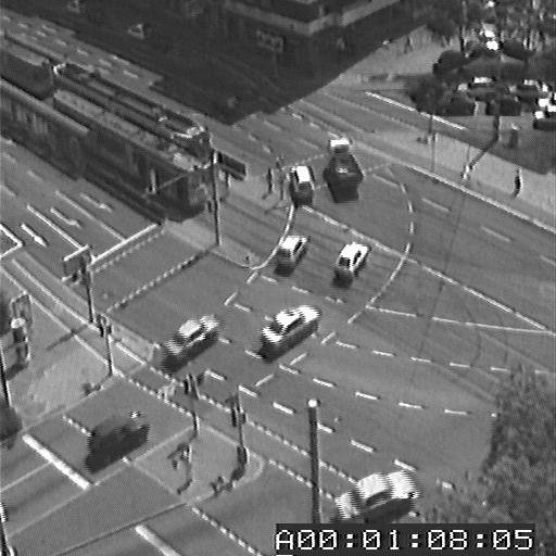
41 Traffic 512x512 (Nagel) max speed: 6.0 pix/frame BA Ours Error map Smoothness error 41


42 Pepsi Can 201x201 (Black) Max speed: 2pix/frame Ours BA Smoothness error 42

 Max")


43 FG: Flower Garden 360x240 (Black) Max speed: 7pix/frame BA LMS Ours Error map Smoothness error 43
44 MPEG Motion Compression Some frames are encoded in terms of others. Independent frame encoded as a still image using JPEG Predicted frame encoded via flow vectors relative to the independent frame and difference image. Between frame encoded using flow vectors and independent and predicted frame. 44
45 MPEG compression method F1 is independent. F4 is predicted. F2 and F3 are between. Each block of I is matched to its closest match in P and represented by a motion vector and a block difference image. Frames B1 and B2 between I and P are represented by two motion vectors per block referring to blocks in F1 and F4. 45
46 Example of compression Assume frames are 512 x 512 bytes, or 32 x 32 blocks of size 16 x 16 pixels. Frame A is ¼ megabytes = 250,000 bytes before JPEG Frame B uses 32 x 32 =1024 motion vectors, or 2048 bytes only if delx and dely are represented as 1 byte integers. 46
47 Segmenting videos Build video segment database Scene change is a change of environment: newsroom to street Shot change is a change of camera view of same scene Camera pan and zoom, as before Fade, dissolve, wipe are used for transitions 47

48 Scene change 48
49 Detect via histogram change (Top) gray level histogram of intensities from frame 1 in newsroom. (Middle) histogram of intensities from frame 2 in newsroom. (Bottom) histogram of intensities from street scene. Histograms change less with pan and zoom of same scene. 49


50 Daniel Gatica Perez s work on describing video content 50

51 Our problem: Finding Video Structure Video Structure: hierarchical description of visual content Table of Contents From thousands of raw frames to video events 51
52 Hierarchical Structure in Video: Extensive Operators Video Sequence Scenes: Semantic Concept. Fair to use? Clusters: Collection of temporally adjacent/visually similar shots Shots: Consecutive frames recorded from a single camera Sequence Scene Cluster Shot Frame 52


53 Daniel s Approach VIDEO SEQUENCE TEMPORAL PARTITION GENERATION VIDEO SHOT FEATURE EXTRACTION PROBABILISTIC HIERARCHICAL CLUSTERING CONSTRUCTION OF VIDEO SEGMENT TREE 53

54 Video Structuring Results (I) 35 shots 9 clusters detected 54
 12 shots 4 clusters")
55 Video Structuring Results (II) 12 shots 4 clusters 55

56 Tree-based Video Representation 56
Lucas-Kanade Motion Estimation. Thanks to Steve Seitz, Simon Baker, Takeo Kanade, and anyone else who helped develop these slides.
 Lucas-Kanade Motion Estimation Thanks to Steve Seitz, Simon Baker, Takeo Kanade, and anyone else who helped develop these slides. 1 Why estimate motion? We live in a 4-D world Wide applications Object
Motion and Optical Flow. Slides from Ce Liu, Steve Seitz, Larry Zitnick, Ali Farhadi
 Motion and Optical Flow Slides from Ce Liu, Steve Seitz, Larry Zitnick, Ali Farhadi We live in a moving world Perceiving, understanding and predicting motion is an important part of our daily lives Motion
CS6670: Computer Vision
 CS6670: Computer Vision Noah Snavely Lecture 19: Optical flow http://en.wikipedia.org/wiki/barberpole_illusion Readings Szeliski, Chapter 8.4-8.5 Announcements Project 2b due Tuesday, Nov 2 Please sign
Motion in 2D image sequences
 Motion in 2D image sequences Definitely used in human vision Object detection and tracking Navigation and obstacle avoidance Analysis of actions or activities Segmentation and understanding of video sequences
VC 11/12 T11 Optical Flow
 VC 11/12 T11 Optical Flow Mestrado em Ciência de Computadores Mestrado Integrado em Engenharia de Redes e Sistemas Informáticos Miguel Tavares Coimbra Outline Optical Flow Constraint Equation Aperture
CS 4495 Computer Vision Motion and Optic Flow
 CS 4495 Computer Vision Aaron Bobick School of Interactive Computing Administrivia PS4 is out, due Sunday Oct 27 th. All relevant lectures posted Details about Problem Set: You may *not* use built in Harris
Automatic Image Alignment (direct) with a lot of slides stolen from Steve Seitz and Rick Szeliski
 with a lot of slides stolen from Steve Seitz and Rick Szeliski") Automatic Image Alignment (direct) with a lot of slides stolen from Steve Seitz and Rick Szeliski 15-463: Computational Photography Alexei Efros, CMU, Fall 2005 Today Go over Midterm Go over Project #3
Automatic Image Alignment (direct) with a lot of slides stolen from Steve Seitz and Rick Szeliski 15-463: Computational Photography Alexei Efros, CMU, Fall 2005 Today Go over Midterm Go over Project #3
Feature Tracking and Optical Flow
 Feature Tracking and Optical Flow Prof. D. Stricker Doz. G. Bleser Many slides adapted from James Hays, Derek Hoeim, Lana Lazebnik, Silvio Saverse, who 1 in turn adapted slides from Steve Seitz, Rick Szeliski,
Lecture 16: Computer Vision
 CS4442/9542b: Artificial Intelligence II Prof. Olga Veksler Lecture 16: Computer Vision Motion Slides are from Steve Seitz (UW), David Jacobs (UMD) Outline Motion Estimation Motion Field Optical Flow Field
Feature Tracking and Optical Flow
 Feature Tracking and Optical Flow Prof. D. Stricker Doz. G. Bleser Many slides adapted from James Hays, Derek Hoeim, Lana Lazebnik, Silvio Saverse, who in turn adapted slides from Steve Seitz, Rick Szeliski,
Lecture 16: Computer Vision
 CS442/542b: Artificial ntelligence Prof. Olga Veksler Lecture 16: Computer Vision Motion Slides are from Steve Seitz (UW), David Jacobs (UMD) Outline Motion Estimation Motion Field Optical Flow Field Methods
Matching. Compare region of image to region of image. Today, simplest kind of matching. Intensities similar.
 Matching Compare region of image to region of image. We talked about this for stereo. Important for motion. Epipolar constraint unknown. But motion small. Recognition Find object in image. Recognize object.
Finally: Motion and tracking. Motion 4/20/2011. CS 376 Lecture 24 Motion 1. Video. Uses of motion. Motion parallax. Motion field
 Finally: Motion and tracking Tracking objects, video analysis, low level motion Motion Wed, April 20 Kristen Grauman UT-Austin Many slides adapted from S. Seitz, R. Szeliski, M. Pollefeys, and S. Lazebnik
EE795: Computer Vision and Intelligent Systems
 EE795: Computer Vision and Intelligent Systems Spring 2012 TTh 17:30-18:45 FDH 204 Lecture 14 130307 http://www.ee.unlv.edu/~b1morris/ecg795/ 2 Outline Review Stereo Dense Motion Estimation Translational
Lecture 19: Motion. Effect of window size 11/20/2007. Sources of error in correspondences. Review Problem set 3. Tuesday, Nov 20
 Lecture 19: Motion Review Problem set 3 Dense stereo matching Sparse stereo matching Indexing scenes Tuesda, Nov 0 Effect of window size W = 3 W = 0 Want window large enough to have sufficient intensit
Peripheral drift illusion
 Peripheral drift illusion Does it work on other animals? Computer Vision Motion and Optical Flow Many slides adapted from J. Hays, S. Seitz, R. Szeliski, M. Pollefeys, K. Grauman and others Video A video
Dense Image-based Motion Estimation Algorithms & Optical Flow
 Dense mage-based Motion Estimation Algorithms & Optical Flow Video A video is a sequence of frames captured at different times The video data is a function of v time (t) v space (x,y) ntroduction to motion
Overview. Video. Overview 4/7/2008. Optical flow. Why estimate motion? Motion estimation: Optical flow. Motion Magnification Colorization.
 Overview Video Optical flow Motion Magnification Colorization Lecture 9 Optical flow Motion Magnification Colorization Overview Optical flow Combination of slides from Rick Szeliski, Steve Seitz, Alyosha
EE795: Computer Vision and Intelligent Systems
 EE795: Computer Vision and Intelligent Systems Spring 2012 TTh 17:30-18:45 FDH 204 Lecture 11 140311 http://www.ee.unlv.edu/~b1morris/ecg795/ 2 Outline Motion Analysis Motivation Differential Motion Optical
Capturing, Modeling, Rendering 3D Structures
 Computer Vision Approach Capturing, Modeling, Rendering 3D Structures Calculate pixel correspondences and extract geometry Not robust Difficult to acquire illumination effects, e.g. specular highlights
Motion and Tracking. Andrea Torsello DAIS Università Ca Foscari via Torino 155, Mestre (VE)
") Motion and Tracking Andrea Torsello DAIS Università Ca Foscari via Torino 155, 30172 Mestre (VE) Motion Segmentation Segment the video into multiple coherently moving objects Motion and Perceptual Organization
Motion and Tracking Andrea Torsello DAIS Università Ca Foscari via Torino 155, 30172 Mestre (VE) Motion Segmentation Segment the video into multiple coherently moving objects Motion and Perceptual Organization
Ninio, J. and Stevens, K. A. (2000) Variations on the Hermann grid: an extinction illusion. Perception, 29,
 Variations on the Hermann grid: an extinction illusion. Perception, 29,") Ninio, J. and Stevens, K. A. (2000) Variations on the Hermann grid: an extinction illusion. Perception, 29, 1209-1217. CS 4495 Computer Vision A. Bobick Sparse to Dense Correspodence Building Rome in
Ninio, J. and Stevens, K. A. (2000) Variations on the Hermann grid: an extinction illusion. Perception, 29, 1209-1217. CS 4495 Computer Vision A. Bobick Sparse to Dense Correspodence Building Rome in
Multi-stable Perception. Necker Cube
 Multi-stable Perception Necker Cube Spinning dancer illusion, Nobuyuki Kayahara Multiple view geometry Stereo vision Epipolar geometry Lowe Hartley and Zisserman Depth map extraction Essential matrix
COMPUTER VISION > OPTICAL FLOW UTRECHT UNIVERSITY RONALD POPPE
 COMPUTER VISION 2017-2018 > OPTICAL FLOW UTRECHT UNIVERSITY RONALD POPPE OUTLINE Optical flow Lucas-Kanade Horn-Schunck Applications of optical flow Optical flow tracking Histograms of oriented flow Assignment
Optical flow and tracking
 EECS 442 Computer vision Optical flow and tracking Intro Optical flow and feature tracking Lucas-Kanade algorithm Motion segmentation Segments of this lectures are courtesy of Profs S. Lazebnik S. Seitz,
Comparison between Motion Analysis and Stereo
 MOTION ESTIMATION The slides are from several sources through James Hays (Brown); Silvio Savarese (U. of Michigan); Octavia Camps (Northeastern); including their own slides. Comparison between Motion Analysis
Motion Estimation. There are three main types (or applications) of motion estimation:
 of motion estimation:") Members: D91922016 朱威達 R93922010 林聖凱 R93922044 謝俊瑋 Motion Estimation There are three main types (or applications) of motion estimation: Parametric motion (image alignment) The main idea of parametric motion
Members: D91922016 朱威達 R93922010 林聖凱 R93922044 謝俊瑋 Motion Estimation There are three main types (or applications) of motion estimation: Parametric motion (image alignment) The main idea of parametric motion
Particle Tracking. For Bulk Material Handling Systems Using DEM Models. By: Jordan Pease
 Particle Tracking For Bulk Material Handling Systems Using DEM Models By: Jordan Pease Introduction Motivation for project Particle Tracking Application to DEM models Experimental Results Future Work References
Computer Vision Lecture 20
 Computer Perceptual Vision and Sensory WS 16/76 Augmented Computing Many slides adapted from K. Grauman, S. Seitz, R. Szeliski, M. Pollefeys, S. Lazebnik Computer Vision Lecture 20 Motion and Optical Flow
Computer Vision Lecture 20
 Computer Perceptual Vision and Sensory WS 16/17 Augmented Computing Computer Perceptual Vision and Sensory WS 16/17 Augmented Computing Computer Perceptual Vision and Sensory WS 16/17 Augmented Computing
Fundamental matrix. Let p be a point in left image, p in right image. Epipolar relation. Epipolar mapping described by a 3x3 matrix F
 Fundamental matrix Let p be a point in left image, p in right image l l Epipolar relation p maps to epipolar line l p maps to epipolar line l p p Epipolar mapping described by a 3x3 matrix F Fundamental
EECS 556 Image Processing W 09
 EECS 556 Image Processing W 09 Motion estimation Global vs. Local Motion Block Motion Estimation Optical Flow Estimation (normal equation) Man slides of this lecture are courtes of prof Milanfar (UCSC)
SURVEY OF LOCAL AND GLOBAL OPTICAL FLOW WITH COARSE TO FINE METHOD
 SURVEY OF LOCAL AND GLOBAL OPTICAL FLOW WITH COARSE TO FINE METHOD M.E-II, Department of Computer Engineering, PICT, Pune ABSTRACT: Optical flow as an image processing technique finds its applications
Lecture 20: Tracking. Tuesday, Nov 27
 Lecture 20: Tracking Tuesday, Nov 27 Paper reviews Thorough summary in your own words Main contribution Strengths? Weaknesses? How convincing are the experiments? Suggestions to improve them? Extensions?
Motion. 1 Introduction. 2 Optical Flow. Sohaib A Khan. 2.1 Brightness Constancy Equation
 Motion Sohaib A Khan 1 Introduction So far, we have dealing with single images of a static scene taken by a fixed camera. Here we will deal with sequence of images taken at different time intervals. Motion
Local Gradient, Global Matching, Piecewise-Smooth Optical Flow
 Local Gradient, Global Matching, Piecewise-Smooth Optical Flow Ming Ye Robert M Haralick Department of Electrical Engineering Department of Computer Science University of Washington CUNY Graduate Center
Marcel Worring Intelligent Sensory Information Systems
 Marcel Worring worring@science.uva.nl Intelligent Sensory Information Systems University of Amsterdam Information and Communication Technology archives of documentaries, film, or training material, video
Optical Flow Estimation
 Optical Flow Estimation Goal: Introduction to image motion and 2D optical flow estimation. Motivation: Motion is a rich source of information about the world: segmentation surface structure from parallax
Visual motion. Many slides adapted from S. Seitz, R. Szeliski, M. Pollefeys
 Visual motion Man slides adapted from S. Seitz, R. Szeliski, M. Pollefes Motion and perceptual organization Sometimes, motion is the onl cue Motion and perceptual organization Sometimes, motion is the
Computer Vision Lecture 20
 Computer Vision Lecture 2 Motion and Optical Flow Bastian Leibe RWTH Aachen http://www.vision.rwth-aachen.de leibe@vision.rwth-aachen.de 28.1.216 Man slides adapted from K. Grauman, S. Seitz, R. Szeliski,
Notes 9: Optical Flow
 Course 049064: Variational Methods in Image Processing Notes 9: Optical Flow Guy Gilboa 1 Basic Model 1.1 Background Optical flow is a fundamental problem in computer vision. The general goal is to find
CS 565 Computer Vision. Nazar Khan PUCIT Lectures 15 and 16: Optic Flow
 CS 565 Computer Vision Nazar Khan PUCIT Lectures 15 and 16: Optic Flow Introduction Basic Problem given: image sequence f(x, y, z), where (x, y) specifies the location and z denotes time wanted: displacement
CS-465 Computer Vision
 CS-465 Computer Vision Nazar Khan PUCIT 9. Optic Flow Optic Flow Nazar Khan Computer Vision 2 / 25 Optic Flow Nazar Khan Computer Vision 3 / 25 Optic Flow Where does pixel (x, y) in frame z move to in
Optic Flow and Motion Detection
 Optic Flow and Motion Detection Computer Vision and Imaging Martin Jagersand Readings: Szeliski Ch 8 Ma, Kosecka, Sastry Ch 4 Image motion Somehow quantify the frame-to to-frame differences in image sequences.
CS664 Lecture #18: Motion
 CS664 Lecture #18: Motion Announcements Most paper choices were fine Please be sure to email me for approval, if you haven t already This is intended to help you, especially with the final project Use
Optical Flow CS 637. Fuxin Li. With materials from Kristen Grauman, Richard Szeliski, S. Narasimhan, Deqing Sun
 Optical Flow CS 637 Fuxin Li With materials from Kristen Grauman, Richard Szeliski, S. Narasimhan, Deqing Sun Motion and perceptual organization Sometimes, motion is the only cue Motion and perceptual
Horn-Schunck and Lucas Kanade 1
 Horn-Schunck and Lucas Kanade 1 Lecture 8 See Sections 4.2 and 4.3 in Reinhard Klette: Concise Computer Vision Springer-Verlag, London, 2014 1 See last slide for copyright information. 1 / 40 Where We
Colour Segmentation-based Computation of Dense Optical Flow with Application to Video Object Segmentation
 ÖGAI Journal 24/1 11 Colour Segmentation-based Computation of Dense Optical Flow with Application to Video Object Segmentation Michael Bleyer, Margrit Gelautz, Christoph Rhemann Vienna University of Technology
Motion estimation. Lihi Zelnik-Manor
 Motion estimation Lihi Zelnik-Manor Optical Flow Where did each piel in image 1 go to in image 2 Optical Flow Pierre Kornprobst's Demo ntroduction Given a video sequence with camera/objects moving we can
Edge and corner detection
 Edge and corner detection Prof. Stricker Doz. G. Bleser Computer Vision: Object and People Tracking Goals Where is the information in an image? How is an object characterized? How can I find measurements
Visual Tracking (1) Tracking of Feature Points and Planar Rigid Objects
 Tracking of Feature Points and Planar Rigid Objects") Intelligent Control Systems Visual Tracking (1) Tracking of Feature Points and Planar Rigid Objects Shingo Kagami Graduate School of Information Sciences, Tohoku University swk(at)ic.is.tohoku.ac.jp http://www.ic.is.tohoku.ac.jp/ja/swk/
Intelligent Control Systems Visual Tracking (1) Tracking of Feature Points and Planar Rigid Objects Shingo Kagami Graduate School of Information Sciences, Tohoku University swk(at)ic.is.tohoku.ac.jp http://www.ic.is.tohoku.ac.jp/ja/swk/
Mariya Zhariy. Uttendorf Introduction to Optical Flow. Mariya Zhariy. Introduction. Determining. Optical Flow. Results. Motivation Definition
 to Constraint to Uttendorf 2005 Contents to Constraint 1 Contents to Constraint 1 2 Constraint Contents to Constraint 1 2 Constraint 3 Visual cranial reflex(vcr)(?) to Constraint Rapidly changing scene
ECE Digital Image Processing and Introduction to Computer Vision
 ECE592-064 Digital Image Processing and Introduction to Computer Vision Depart. of ECE, NC State University Instructor: Tianfu (Matt) Wu Spring 2017 Recap, SIFT Motion Tracking Change Detection Feature
Fi#ng & Matching Region Representa3on Image Alignment, Op3cal Flow
 Fi#ng & Matching Region Representa3on Image Alignment, Op3cal Flow Lectures 5 & 6 Prof. Fergus Slides from: S. Lazebnik, S. Seitz, M. Pollefeys, A. Effros. Facebook 360 photos Panoramas How do we build
Comparison Between The Optical Flow Computational Techniques
 Comparison Between The Optical Flow Computational Techniques Sri Devi Thota #1, Kanaka Sunanda Vemulapalli* 2, Kartheek Chintalapati* 3, Phanindra Sai Srinivas Gudipudi* 4 # Associate Professor, Dept.
Leow Wee Kheng CS4243 Computer Vision and Pattern Recognition. Motion Tracking. CS4243 Motion Tracking 1
 Leow Wee Kheng CS4243 Computer Vision and Pattern Recognition Motion Tracking CS4243 Motion Tracking 1 Changes are everywhere! CS4243 Motion Tracking 2 Illumination change CS4243 Motion Tracking 3 Shape
Visual Tracking. Image Processing Laboratory Dipartimento di Matematica e Informatica Università degli studi di Catania.
 Image Processing Laboratory Dipartimento di Matematica e Informatica Università degli studi di Catania 1 What is visual tracking? estimation of the target location over time 2 applications Six main areas:
Computer Vision II Lecture 4
 Computer Vision II Lecture 4 Color based Tracking 29.04.2014 Bastian Leibe RWTH Aachen http://www.vision.rwth-aachen.de leibe@vision.rwth-aachen.de Course Outline Single-Object Tracking Background modeling
Displacement estimation
 Displacement estimation Displacement estimation by block matching" l Search strategies" l Subpixel estimation" Gradient-based displacement estimation ( optical flow )" l Lukas-Kanade" l Multi-scale coarse-to-fine"
Local Feature Detectors
 Local Feature Detectors Selim Aksoy Department of Computer Engineering Bilkent University saksoy@cs.bilkent.edu.tr Slides adapted from Cordelia Schmid and David Lowe, CVPR 2003 Tutorial, Matthew Brown,
Visual Tracking. Antonino Furnari. Image Processing Lab Dipartimento di Matematica e Informatica Università degli Studi di Catania
 Visual Tracking Antonino Furnari Image Processing Lab Dipartimento di Matematica e Informatica Università degli Studi di Catania furnari@dmi.unict.it 11 giugno 2015 What is visual tracking? estimation
Robust Camera Pan and Zoom Change Detection Using Optical Flow
 Robust Camera and Change Detection Using Optical Flow Vishnu V. Makkapati Philips Research Asia - Bangalore Philips Innovation Campus, Philips Electronics India Ltd. Manyata Tech Park, Nagavara, Bangalore
Computer Vision for HCI. Motion. Motion
 Computer Vision for HCI Motion Motion Changing scene may be observed in a sequence of images Changing pixels in image sequence provide important features for object detection and activity recognition 2
Ruch (Motion) Rozpoznawanie Obrazów Krzysztof Krawiec Instytut Informatyki, Politechnika Poznańska. Krzysztof Krawiec IDSS
 Rozpoznawanie Obrazów Krzysztof Krawiec Instytut Informatyki, Politechnika Poznańska. Krzysztof Krawiec IDSS") Ruch (Motion) Rozpoznawanie Obrazów Krzysztof Krawiec Instytut Informatyki, Politechnika Poznańska 1 Krzysztof Krawiec IDSS 2 The importance of visual motion Adds entirely new (temporal) dimension to visual
Ruch (Motion) Rozpoznawanie Obrazów Krzysztof Krawiec Instytut Informatyki, Politechnika Poznańska 1 Krzysztof Krawiec IDSS 2 The importance of visual motion Adds entirely new (temporal) dimension to visual
BSB663 Image Processing Pinar Duygulu. Slides are adapted from Selim Aksoy
 BSB663 Image Processing Pinar Duygulu Slides are adapted from Selim Aksoy Image matching Image matching is a fundamental aspect of many problems in computer vision. Object or scene recognition Solving
Mixture Models and EM
 Mixture Models and EM Goal: Introduction to probabilistic mixture models and the expectationmaximization (EM) algorithm. Motivation: simultaneous fitting of multiple model instances unsupervised clustering
Coarse-to-fine image registration
 Today we will look at a few important topics in scale space in computer vision, in particular, coarseto-fine approaches, and the SIFT feature descriptor. I will present only the main ideas here to give
Computer Vision 2. SS 18 Dr. Benjamin Guthier Professur für Bildverarbeitung. Computer Vision 2 Dr. Benjamin Guthier
 Computer Vision 2 SS 18 Dr. Benjamin Guthier Professur für Bildverarbeitung Computer Vision 2 Dr. Benjamin Guthier 1. IMAGE PROCESSING Computer Vision 2 Dr. Benjamin Guthier Content of this Chapter Non-linear
Representing Moving Images with Layers. J. Y. Wang and E. H. Adelson MIT Media Lab
 Representing Moving Images with Layers J. Y. Wang and E. H. Adelson MIT Media Lab Goal Represent moving images with sets of overlapping layers Layers are ordered in depth and occlude each other Velocity
CSE 252A Computer Vision Homework 3 Instructor: Ben Ochoa Due : Monday, November 21, 2016, 11:59 PM
 CSE 252A Computer Vision Homework 3 Instructor: Ben Ochoa Due : Monday, November 21, 2016, 11:59 PM Instructions: Homework 3 has to be submitted in groups of 3. Review the academic integrity and collaboration
Adaptive Multi-Stage 2D Image Motion Field Estimation
 Adaptive Multi-Stage 2D Image Motion Field Estimation Ulrich Neumann and Suya You Computer Science Department Integrated Media Systems Center University of Southern California, CA 90089-0781 ABSRAC his
Searching Video Collections:Part I
 Searching Video Collections:Part I Introduction to Multimedia Information Retrieval Multimedia Representation Visual Features (Still Images and Image Sequences) Color Texture Shape Edges Objects, Motion
CS201: Computer Vision Introduction to Tracking
 CS201: Computer Vision Introduction to Tracking John Magee 18 November 2014 Slides courtesy of: Diane H. Theriault Question of the Day How can we represent and use motion in images? 1 What is Motion? Change
Chaplin, Modern Times, 1936
 Chaplin, Modern Times, 1936 [A Bucket of Water and a Glass Matte: Special Effects in Modern Times; bonus feature on The Criterion Collection set] Multi-view geometry problems Structure: Given projections
CS231A Section 6: Problem Set 3
 CS231A Section 6: Problem Set 3 Kevin Wong Review 6 -! 1 11/09/2012 Announcements PS3 Due 2:15pm Tuesday, Nov 13 Extra Office Hours: Friday 6 8pm Huang Common Area, Basement Level. Review 6 -! 2 Topics
Digital Image Processing COSC 6380/4393
 Digital Image Processing COSC 6380/4393 Lecture 21 Nov 16 th, 2017 Pranav Mantini Ack: Shah. M Image Processing Geometric Transformation Point Operations Filtering (spatial, Frequency) Input Restoration/
CPSC 425: Computer Vision
 1 / 49 CPSC 425: Computer Vision Instructor: Fred Tung ftung@cs.ubc.ca Department of Computer Science University of British Columbia Lecture Notes 2015/2016 Term 2 2 / 49 Menu March 10, 2016 Topics: Motion
Visual Tracking (1) Pixel-intensity-based methods
 Pixel-intensity-based methods") Intelligent Control Systems Visual Tracking (1) Pixel-intensity-based methods Shingo Kagami Graduate School of Information Sciences, Tohoku University swk(at)ic.is.tohoku.ac.jp http://www.ic.is.tohoku.ac.jp/ja/swk/
Intelligent Control Systems Visual Tracking (1) Pixel-intensity-based methods Shingo Kagami Graduate School of Information Sciences, Tohoku University swk(at)ic.is.tohoku.ac.jp http://www.ic.is.tohoku.ac.jp/ja/swk/
Final Exam Study Guide
 Final Exam Study Guide Exam Window: 28th April, 12:00am EST to 30th April, 11:59pm EST Description As indicated in class the goal of the exam is to encourage you to review the material from the course.
LOCAL-GLOBAL OPTICAL FLOW FOR IMAGE REGISTRATION
 LOCAL-GLOBAL OPTICAL FLOW FOR IMAGE REGISTRATION Ammar Zayouna Richard Comley Daming Shi Middlesex University School of Engineering and Information Sciences Middlesex University, London NW4 4BT, UK A.Zayouna@mdx.ac.uk
The Template Update Problem
 The Template Update Problem Iain Matthews, Takahiro Ishikawa, and Simon Baker The Robotics Institute Carnegie Mellon University Abstract Template tracking dates back to the 1981 Lucas-Kanade algorithm.
Optic Flow and Basics Towards Horn-Schunck 1
 Optic Flow and Basics Towards Horn-Schunck 1 Lecture 7 See Section 4.1 and Beginning of 4.2 in Reinhard Klette: Concise Computer Vision Springer-Verlag, London, 2014 1 See last slide for copyright information.
CSCI 1290: Comp Photo
 CSCI 1290: Comp Photo Fall 2018 @ Brown University James Tompkin Many slides thanks to James Hays old CS 129 course, along with all its acknowledgements. CS 4495 Computer Vision A. Bobick Motion and Optic
Robert Collins CSE598G. Intro to Template Matching and the Lucas-Kanade Method
 Intro to Template Matching and the Lucas-Kanade Method Appearance-Based Tracking current frame + previous location likelihood over object location current location appearance model (e.g. image template,
Module 7 VIDEO CODING AND MOTION ESTIMATION
 Module 7 VIDEO CODING AND MOTION ESTIMATION Lesson 20 Basic Building Blocks & Temporal Redundancy Instructional Objectives At the end of this lesson, the students should be able to: 1. Name at least five
Feature Based Registration - Image Alignment
 Feature Based Registration - Image Alignment Image Registration Image registration is the process of estimating an optimal transformation between two or more images. Many slides from Alexei Efros http://graphics.cs.cmu.edu/courses/15-463/2007_fall/463.html
Video Alignment. Literature Survey. Spring 2005 Prof. Brian Evans Multidimensional Digital Signal Processing Project The University of Texas at Austin
 Literature Survey Spring 2005 Prof. Brian Evans Multidimensional Digital Signal Processing Project The University of Texas at Austin Omer Shakil Abstract This literature survey compares various methods
Feature Detectors and Descriptors: Corners, Lines, etc.
 Feature Detectors and Descriptors: Corners, Lines, etc. Edges vs. Corners Edges = maxima in intensity gradient Edges vs. Corners Corners = lots of variation in direction of gradient in a small neighborhood
Introduction to Computer Vision
 Introduction to Computer Vision Michael J. Black Oct 2009 Motion estimation Goals Motion estimation Affine flow Optimization Large motions Why affine? Monday dense, smooth motion and regularization. Robust
The Lucas & Kanade Algorithm
 The Lucas & Kanade Algorithm Instructor - Simon Lucey 16-423 - Designing Computer Vision Apps Today Registration, Registration, Registration. Linearizing Registration. Lucas & Kanade Algorithm. 3 Biggest
Chapter 3 Image Registration. Chapter 3 Image Registration
 Chapter 3 Image Registration Distributed Algorithms for Introduction (1) Definition: Image Registration Input: 2 images of the same scene but taken from different perspectives Goal: Identify transformation
Global Flow Estimation. Lecture 9
 Motion Models Image Transformations to relate two images 3D Rigid motion Perspective & Orthographic Transformation Planar Scene Assumption Transformations Translation Rotation Rigid Affine Homography Pseudo
Optical flow. Cordelia Schmid
 Optical flow Cordelia Schmid Motion field The motion field is the projection of the 3D scene motion into the image Optical flow Definition: optical flow is the apparent motion of brightness patterns in
Announcements. Computer Vision I. Motion Field Equation. Revisiting the small motion assumption. Visual Tracking. CSE252A Lecture 19.
 Visual Tracking CSE252A Lecture 19 Hw 4 assigned Announcements No class on Thursday 12/6 Extra class on Tuesday 12/4 at 6:30PM in WLH Room 2112 Motion Field Equation Measurements I x = I x, T: Components
Multimedia Retrieval Ch 5 Image Processing. Anne Ylinen
 Multimedia Retrieval Ch 5 Image Processing Anne Ylinen Agenda Types of image processing Application areas Image analysis Image features Types of Image Processing Image Acquisition Camera Scanners X-ray
Global Flow Estimation. Lecture 9
 Global Flow Estimation Lecture 9 Global Motion Estimate motion using all pixels in the image. Parametric flow gives an equation, which describes optical flow for each pixel. Affine Projective Global motion
Motion Estimation (II) Ce Liu Microsoft Research New England
 Ce Liu Microsoft Research New England") Motion Estimation (II) Ce Liu celiu@microsoft.com Microsoft Research New England Last time Motion perception Motion representation Parametric motion: Lucas-Kanade T I x du dv = I x I T x I y I x T I y
Motion Estimation (II) Ce Liu celiu@microsoft.com Microsoft Research New England Last time Motion perception Motion representation Parametric motion: Lucas-Kanade T I x du dv = I x I T x I y I x T I y
Applications. Foreground / background segmentation Finding skin-colored regions. Finding the moving objects. Intelligent scissors
 Segmentation I Goal Separate image into coherent regions Berkeley segmentation database: http://www.eecs.berkeley.edu/research/projects/cs/vision/grouping/segbench/ Slide by L. Lazebnik Applications Intelligent
Video Alignment. Final Report. Spring 2005 Prof. Brian Evans Multidimensional Digital Signal Processing Project The University of Texas at Austin
 Final Report Spring 2005 Prof. Brian Evans Multidimensional Digital Signal Processing Project The University of Texas at Austin Omer Shakil Abstract This report describes a method to align two videos.
Classification and Detection in Images. D.A. Forsyth
 Classification and Detection in Images D.A. Forsyth Classifying Images Motivating problems detecting explicit images classifying materials classifying scenes Strategy build appropriate image features train