CS 565 Computer Vision. Nazar Khan PUCIT Lectures 15 and 16: Optic Flow
|
|
|
- Kelley Cobb
- 5 years ago
- Views:
Transcription
1 CS 565 Computer Vision Nazar Khan PUCIT Lectures 15 and 16: Optic Flow
2 Introduction Basic Problem given: image sequence f(x, y, z), where (x, y) specifies the location and z denotes time wanted: displacement vector field of the image structures: optic flow (u(x,y,z),v(x,y,z)) T Basically, where does pixel (x,y) move from frame z to frame z+1. Such correspondence problems are key problems in computer vision. Similar Correspondence Problems computing the displacements (disparities) between the two images of a stereo pair matching (registration) of medical images that are obtained with different modalities, parameter settings or at different times
3 Introduction What is Optic Flow Good for? recognition of moving pedestrians in driver assistant systems estimation of motion parameters in robotics reconstruction of the 3-D world from an image sequence (structure-from-motion) tracking of moving objects, e.g. human body motion video processing, e.g. frame interpolation efficient video coding
4
5 Grey Value Constancy Assumption Corresponding image structures should have the same grey value. Thus, the optic flow between frame z and z + 1 satisfies f(x+u, y+v, z+1) = f(x, y, z). Unfortunately the unknown flow field (u, v) T is not directly accessible. This problem is similar to the Harris corner detection formulation where direction d was also not accessible. (How did we get around that problem?)
6 Linearisation by Taylor Expansion Let us assume that (u, v) is small and f varies slowly. Then a Taylor expansion around (x, y, z) gives a good approximation 0 = f(x+u, y+v, z+1) - f(x, y, z) f(x, y, z) + f x (x, y, z) u + f y (x, y, z) v + f z (x, y, z) - f(x, y, z) = f x (x, y, z) u + f y (x, y, z) v + f z (x, y, z) (H.W. Prove this.) where subscripts denote partial derivatives. This yields the linearised optic flow constraint (OFC) f x u + f y v + f z = 0 where the unknown flow field (u, v) T is directly accessible.
7 Assumptions We have made 2 assumptions so far: 1. Grey value constancy 2. Linearised OFC
8 How Realistic are These Assumptions? The grey value constancy assumption is often surprisingly realistic: Many illumination changes happen very slowly, i.e. over many frames. More complicated models exist that take into account illumination changes. The linearisation assumption is violated more frequently: Conventional video cameras often suffer from temporal undersampling (produce displacements over several pixels) while Taylor expansion is accurate only for small displacements. Remedies: use original OFC without linearisation (model becomes more difficult) spatial downsampling (after lowpass filtering!) (H.W. How will this help?)
9 The Aperture Problem The OFC f x u + f y v + f z = 0 is one equation in two unknowns u, v. Thus, it cannot have a unique solution. The OFC specifies only the flow component parallel to the spatial gradient f = (f x, f y ) T : 0 = f x u + f y v + f z = [u v] f + f z This sheds more light on the non-uniqueness problem: Adding arbitrary flow components orthogonal to f does not violate the OFC. This is called aperture problem. Within the viewing circle (aperture), movements in A, B and C will appear the same even though the real movements are all different.
10 The Aperture Problem Additional assumptions are necessary to get a unique solution. Specifying different additional constraints leads to different methods. Let us first analyse the flow component along f.
11 The Normal Flow Expressing the flow vector (u, v) T in terms of the basis vectors n= f/ f and t= f / f gives the flow normal and tangential to the edge of f: (u,v) T = (u, v) f/ f f/ f + (u, v) f / f f / f =: (u n,v n ) T + (u t,v t ) T. The OFC yields (u, v) f = f z, and the normal flow becomes (u n,v n ) T = - f z / f. f/ f = -1/(f x2 +f y2 ) (f x f z,f y f z ) T The normal flow is the only flow that can be computed from the OFC without additional constraints. Unfortunately, it gives poor results.

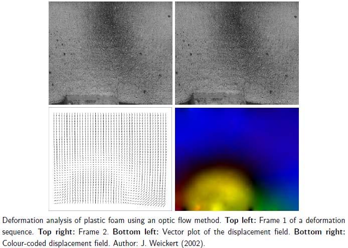
12 Hamburg Taxi Sequence
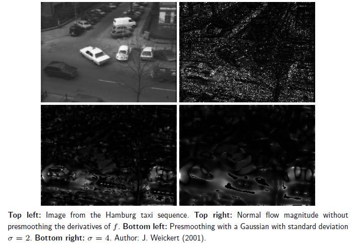
13
14 The Spatial Approach of Lucas and Kanade Additional assumption for dealing with the aperture problem: The optic flow in (x 0, y 0 ) at time z 0 can be approximated by a constant vector (u, v) within some disk-shaped neighbourhood B(x 0, y 0 ) of radius ρ. least squares model: flow in (x 0, y 0 ) minimises the local energy
15 The Spatial Approach of Lucas and Kanade least squares model: flow in (x 0, y 0 ) minimises the local energy Computing partial derivatives and equating to 0
16 The Spatial Approach of Lucas and Kanade The unknowns u and v are constants that can be moved out of the integral. This yields the linear system Multiplying both sides by 1/ B ρ does not change the linear system. 1/ B ρ can be multiplied with each integral on both sides. So the integrals convert to averages. Averaging can be replaced by weighted averaging. One form of weighted averaging is Gaussian smoothing.
17 The Spatial Approach of Lucas and Kanade Often one replaces the box filter with a hard window B(x, y) by a smooth convolution with a Gaussian K ρ : Thus, the Lucas Kanade method solves a 2 2 linear system of equations. The (spatial) structure tensor J ρ serves as system matrix.
18 The Spatial Approach of Lucas and Kanade Thus, the Lucas Kanade method solves a 2 2 linear system of equations. The (spatial) structure tensor J ρ serves as system matrix.

19
20 The Spatial Approach of Lucas and Kanade When Does the Linear System Have No Unique Solution? rank(j) = 0 (two vanishing eigenvalues): Happens if the spatial gradient vanishes in the entire neighbourhood. Nothing can be said in this case. Simple criterion: trace (J) = j 1,1 + j 2,2 ε. (Remember that J is positive semidefinite)
21 The Spatial Approach of Lucas and Kanade When Does the Linear System Have No Unique Solution? rank(j) = 1 (one vanishing eigenvalue): Happens if we have the same (nonvanishing) spatial gradient within the entire neighbourhood. Then both equations are linearly dependent (infinitely many solutions). Simple criterion: det (J) = j 1,1 j 2,2 j 1,22 ε (while trace(j) > ε). In this case the aperture problem persists. One can only compute the normal flow (u n,v n ) T = -1/(f x2 +f y2 ) (f x f z,f y f z ) T

22 The Spatial Approach of Lucas and Kanade
23 The Spatial Approach of Lucas and Kanade Advantages simple and fast method requires only two frames (low memory requirements) good value for money: results often superior to more complicated approaches Disadvantages problems at locations where the local constancy assumption is violated: flow discontinuities and nontranslatory motion (e.g. rotation) local method that does not allow to compute the flow field at all locations
24 The Spatiotemporal Approach of Biguen et al. Optic flow is regarded as orientation in the space time domain and formulated as a principal component analysis problem of the structure tensor. We search for the direction with the least grey value changes within a 3-D ball-shaped neighbourhood B(x 0,y 0,z 0 ) of radius ρ.
25 The Spatiotemporal Approach of Biguen et al. It is given by the unit vector w=(w 1,w 2,w 3 ) T that minimises When re-normalising the third component of the optimal w to 1, the first two components give the optic flow: u = w 1 /w 3, v = w 2 /w 3
26 The Spatiotemporal Approach of Biguen et al. Using the spatiotemporal gradient notation 3 f := (f x, f y, f z ) T one minimises with the constraint w =1
27 The Spatiotemporal Approach of Biguen et al. The desired vector w is the normalised eigenvector to the smallest eigenvalue of Summation in region B ρ can be replaced by Gaussian convolution. Leads to a principal component analysis of the spatiotemporal structure tensor
28 The Spatiotemporal Approach of Biguen et al. Flow Classification with the Eigenvalues of the Structure Tensor Let μ 1 μ 2 μ 3 0 be the eigenvalues of J ρ. rank(j) = 0 (three vanishing eigenvalues): If tr J = j 1,1 + j 2,2 + j 3,3 τ 1, nothing can be said: The gradients are too small. rank(j) = 3 (no vanishing eigenvalues): If μ 3 τ 2, then the assumption of a locally constant flow is violated. Either a flow discontinuity or noise dominates. rank(j) = 1 (two vanishing eigenvalues): If μ 2 τ 3, we have two low-contrast eigendirections. No unique flow exists (aperture problem). One can compute the normal flow only. rank(j) = 2 (one vanishing eigenvalue): In this case the optic flow results from the eigenvector w to the smallest eigenvalue μ 3. Normalising its third component to 1, the first two components give u and v.
29 The Spatiotemporal Approach of Biguen et al.
30 The Spatiotemporal Approach of Biguen et al. Advantages high robustness with respect to noise good results for translatory motion eigenvalues of the spatiotemporal structure tensors provide detailed information on the optic flow Disadvantages more complicated than Lucas Kanade: numerical principal component analysis of a 3 3 matrix problems at flow discontinuities and locations with non-translatory motion (e.g. rotation) local method that does not give full flow fields several threshold parameters
31 Summary of Local Optic Flow Methods Assuming grey value constancy leads to the Optic Flow Constraint (OFC). It allows to compute the normal flow only (aperture problem). Computing the full flow requires additional assumptions. Lucas and Kanade assume a locally constant flow (in 2D). This yields a linear system of equations with the spatial structure tensor as system matrix.
32 Summary of Local Optic Flow Methods The method of Biguen et al. estimates the flow as orientation in the spatiotemporal domain. It leads to a principal component analysis problem of the spatiotemporal structure tensor. Both are local methods that do not compute the flow at every pixel. That is, the flow field is not dense.
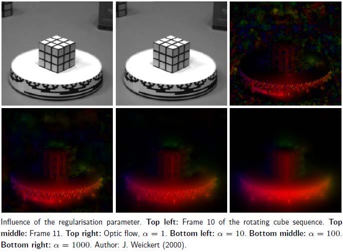
33 Variational Method of Horn and Schunck At some given time z the optic flow field is determined as minimising the function (u(x, y), v(x, y)) T of the energy functional Has a unique solution that depends continuously on the image data.
34 Variational Method of Horn and Schunck Regularisation parameter α>0 determines smoothness of the flow field: α 0 yields the normal flow. The larger α, the smoother the flow field.

35 Optic flow computation using the Horn Schunck method. Top left: Frame 10 of a synthetic image sequence. Top right: Frame 11. Bottom left: Optic flow, vector plot. Bottom right: Optic flow, colour-coded. Author: J. Weickert (2000).
36
37 Variational Method of Horn and Schunck Main advantage Dense flow fields due to filling-in effect: At locations, where no reliable flow estimation is possible (small f ), the smoothness term dominates over the data term. This propagates data from the neighbourhood. No additional threshold parameters necessary
38 How to solve for the flow field (u,v)? Step 1: Going to the Euler-Lagrange Equations
39 How to solve for the flow field (u,v)?
40 How to solve for the flow field (u,v)?
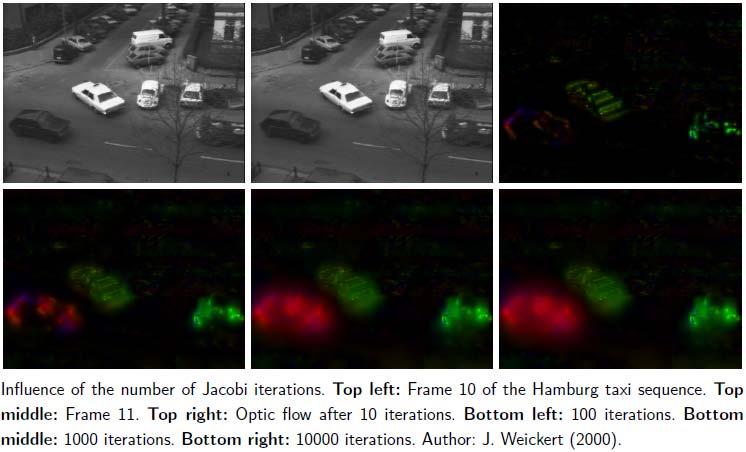
41 How to solve for the flow field (u,v)? Step 2: Discretisation Approximate required first and second order derivatives using simple difference operators. Yields the difference equations for all pixels (i=1,,n) where h is the grid size (usually 1). Can be written as a sparse but very large linear system Bx=d. Size of B will be 69GB for a 256x256 image!
42 How to solve for the flow field (u,v)? Step 3: Solving the Linear System Jacobi Method: Iterative way of solving Bx=d 1. Let B=D N with a diagonal matrix D and a remainder N. 2. Then the problem Dx = Nx + d is solved iteratively using x (k+1) = D 1 (Nx (k) + d) low computational effort per iteration if B is sparse: 1 matrix vector product, 1 vector addition, 1 vector scaling only small additional memory requirement: vector x (k) well-suited for parallel computing residue r (k) := Bx (k) d allows simple stopping criterion: stop if r (k) / r (0) <ε
43 How to solve for the flow field (u,v)? All of the above boils down to a very simple iterative scheme with k = 0, 1, 2,... and an arbitrary initialisation (e.g. null vector). All of you can implement this easily! (Assignment 5)
44 Flow estimate at pixel j at iteration k Flow estimate at pixel i at iteration k Flow estimate at pixel i at iteration k+1 h=grid distance (usually h=1) α=smoothness parameter N(i)=set of neighboring pixels of pixel i f xi, f yi, f zi = spatial and temporal gradients at pixel i.
45
46 Summary of Global Optic Flow Methods Variational methods for computing the optic flow are global methods. Create dense flow fields by filling-in Model assumptions of the variational Horn and Schunck approach: 1. grey value constancy, 2. smoothness of the flow field Mathematically well-founded
47 Summary of Global Optic Flow Methods Minimising the energy functional leads to coupled differential equations. Discretisation creates a large, sparse linear system of equations. can be solved iteratively, e.g. using the Jacobi method Variational methods can be extended and generalised in numerous ways, both with respect to models and to algorithms.
CS-465 Computer Vision
 CS-465 Computer Vision Nazar Khan PUCIT 9. Optic Flow Optic Flow Nazar Khan Computer Vision 2 / 25 Optic Flow Nazar Khan Computer Vision 3 / 25 Optic Flow Where does pixel (x, y) in frame z move to in
COMPUTER VISION > OPTICAL FLOW UTRECHT UNIVERSITY RONALD POPPE
 COMPUTER VISION 2017-2018 > OPTICAL FLOW UTRECHT UNIVERSITY RONALD POPPE OUTLINE Optical flow Lucas-Kanade Horn-Schunck Applications of optical flow Optical flow tracking Histograms of oriented flow Assignment
CS664 Lecture #18: Motion
 CS664 Lecture #18: Motion Announcements Most paper choices were fine Please be sure to email me for approval, if you haven t already This is intended to help you, especially with the final project Use
Feature Tracking and Optical Flow
 Feature Tracking and Optical Flow Prof. D. Stricker Doz. G. Bleser Many slides adapted from James Hays, Derek Hoeim, Lana Lazebnik, Silvio Saverse, who 1 in turn adapted slides from Steve Seitz, Rick Szeliski,
Motion. 1 Introduction. 2 Optical Flow. Sohaib A Khan. 2.1 Brightness Constancy Equation
 Motion Sohaib A Khan 1 Introduction So far, we have dealing with single images of a static scene taken by a fixed camera. Here we will deal with sequence of images taken at different time intervals. Motion
Leow Wee Kheng CS4243 Computer Vision and Pattern Recognition. Motion Tracking. CS4243 Motion Tracking 1
 Leow Wee Kheng CS4243 Computer Vision and Pattern Recognition Motion Tracking CS4243 Motion Tracking 1 Changes are everywhere! CS4243 Motion Tracking 2 Illumination change CS4243 Motion Tracking 3 Shape
CS 4495 Computer Vision Motion and Optic Flow
 CS 4495 Computer Vision Aaron Bobick School of Interactive Computing Administrivia PS4 is out, due Sunday Oct 27 th. All relevant lectures posted Details about Problem Set: You may *not* use built in Harris
Peripheral drift illusion
 Peripheral drift illusion Does it work on other animals? Computer Vision Motion and Optical Flow Many slides adapted from J. Hays, S. Seitz, R. Szeliski, M. Pollefeys, K. Grauman and others Video A video
Mariya Zhariy. Uttendorf Introduction to Optical Flow. Mariya Zhariy. Introduction. Determining. Optical Flow. Results. Motivation Definition
 to Constraint to Uttendorf 2005 Contents to Constraint 1 Contents to Constraint 1 2 Constraint Contents to Constraint 1 2 Constraint 3 Visual cranial reflex(vcr)(?) to Constraint Rapidly changing scene
Lucas-Kanade Motion Estimation. Thanks to Steve Seitz, Simon Baker, Takeo Kanade, and anyone else who helped develop these slides.
 Lucas-Kanade Motion Estimation Thanks to Steve Seitz, Simon Baker, Takeo Kanade, and anyone else who helped develop these slides. 1 Why estimate motion? We live in a 4-D world Wide applications Object
Horn-Schunck and Lucas Kanade 1
 Horn-Schunck and Lucas Kanade 1 Lecture 8 See Sections 4.2 and 4.3 in Reinhard Klette: Concise Computer Vision Springer-Verlag, London, 2014 1 See last slide for copyright information. 1 / 40 Where We
Motion Estimation. There are three main types (or applications) of motion estimation:
 of motion estimation:") Members: D91922016 朱威達 R93922010 林聖凱 R93922044 謝俊瑋 Motion Estimation There are three main types (or applications) of motion estimation: Parametric motion (image alignment) The main idea of parametric motion
Members: D91922016 朱威達 R93922010 林聖凱 R93922044 謝俊瑋 Motion Estimation There are three main types (or applications) of motion estimation: Parametric motion (image alignment) The main idea of parametric motion
Feature Tracking and Optical Flow
 Feature Tracking and Optical Flow Prof. D. Stricker Doz. G. Bleser Many slides adapted from James Hays, Derek Hoeim, Lana Lazebnik, Silvio Saverse, who in turn adapted slides from Steve Seitz, Rick Szeliski,
Dense Image-based Motion Estimation Algorithms & Optical Flow
 Dense mage-based Motion Estimation Algorithms & Optical Flow Video A video is a sequence of frames captured at different times The video data is a function of v time (t) v space (x,y) ntroduction to motion
CS6670: Computer Vision
 CS6670: Computer Vision Noah Snavely Lecture 19: Optical flow http://en.wikipedia.org/wiki/barberpole_illusion Readings Szeliski, Chapter 8.4-8.5 Announcements Project 2b due Tuesday, Nov 2 Please sign
EECS 556 Image Processing W 09
 EECS 556 Image Processing W 09 Motion estimation Global vs. Local Motion Block Motion Estimation Optical Flow Estimation (normal equation) Man slides of this lecture are courtes of prof Milanfar (UCSC)
Finally: Motion and tracking. Motion 4/20/2011. CS 376 Lecture 24 Motion 1. Video. Uses of motion. Motion parallax. Motion field
 Finally: Motion and tracking Tracking objects, video analysis, low level motion Motion Wed, April 20 Kristen Grauman UT-Austin Many slides adapted from S. Seitz, R. Szeliski, M. Pollefeys, and S. Lazebnik
Visual Tracking (1) Feature Point Tracking and Block Matching
 Feature Point Tracking and Block Matching") Intelligent Control Systems Visual Tracking (1) Feature Point Tracking and Block Matching Shingo Kagami Graduate School of Information Sciences, Tohoku University swk(at)ic.is.tohoku.ac.jp http://www.ic.is.tohoku.ac.jp/ja/swk/
Intelligent Control Systems Visual Tracking (1) Feature Point Tracking and Block Matching Shingo Kagami Graduate School of Information Sciences, Tohoku University swk(at)ic.is.tohoku.ac.jp http://www.ic.is.tohoku.ac.jp/ja/swk/
EE795: Computer Vision and Intelligent Systems
 EE795: Computer Vision and Intelligent Systems Spring 2012 TTh 17:30-18:45 FDH 204 Lecture 11 140311 http://www.ee.unlv.edu/~b1morris/ecg795/ 2 Outline Motion Analysis Motivation Differential Motion Optical
EE795: Computer Vision and Intelligent Systems
 EE795: Computer Vision and Intelligent Systems Spring 2012 TTh 17:30-18:45 FDH 204 Lecture 14 130307 http://www.ee.unlv.edu/~b1morris/ecg795/ 2 Outline Review Stereo Dense Motion Estimation Translational
Notes 9: Optical Flow
 Course 049064: Variational Methods in Image Processing Notes 9: Optical Flow Guy Gilboa 1 Basic Model 1.1 Background Optical flow is a fundamental problem in computer vision. The general goal is to find
Capturing, Modeling, Rendering 3D Structures
 Computer Vision Approach Capturing, Modeling, Rendering 3D Structures Calculate pixel correspondences and extract geometry Not robust Difficult to acquire illumination effects, e.g. specular highlights
Visual Tracking (1) Tracking of Feature Points and Planar Rigid Objects
 Tracking of Feature Points and Planar Rigid Objects") Intelligent Control Systems Visual Tracking (1) Tracking of Feature Points and Planar Rigid Objects Shingo Kagami Graduate School of Information Sciences, Tohoku University swk(at)ic.is.tohoku.ac.jp http://www.ic.is.tohoku.ac.jp/ja/swk/
Intelligent Control Systems Visual Tracking (1) Tracking of Feature Points and Planar Rigid Objects Shingo Kagami Graduate School of Information Sciences, Tohoku University swk(at)ic.is.tohoku.ac.jp http://www.ic.is.tohoku.ac.jp/ja/swk/
Matching. Compare region of image to region of image. Today, simplest kind of matching. Intensities similar.
 Matching Compare region of image to region of image. We talked about this for stereo. Important for motion. Epipolar constraint unknown. But motion small. Recognition Find object in image. Recognize object.
Motion and Optical Flow. Slides from Ce Liu, Steve Seitz, Larry Zitnick, Ali Farhadi
 Motion and Optical Flow Slides from Ce Liu, Steve Seitz, Larry Zitnick, Ali Farhadi We live in a moving world Perceiving, understanding and predicting motion is an important part of our daily lives Motion
Lecture 19: Motion. Effect of window size 11/20/2007. Sources of error in correspondences. Review Problem set 3. Tuesday, Nov 20
 Lecture 19: Motion Review Problem set 3 Dense stereo matching Sparse stereo matching Indexing scenes Tuesda, Nov 0 Effect of window size W = 3 W = 0 Want window large enough to have sufficient intensit
Optic Flow and Basics Towards Horn-Schunck 1
 Optic Flow and Basics Towards Horn-Schunck 1 Lecture 7 See Section 4.1 and Beginning of 4.2 in Reinhard Klette: Concise Computer Vision Springer-Verlag, London, 2014 1 See last slide for copyright information.
VC 11/12 T11 Optical Flow
 VC 11/12 T11 Optical Flow Mestrado em Ciência de Computadores Mestrado Integrado em Engenharia de Redes e Sistemas Informáticos Miguel Tavares Coimbra Outline Optical Flow Constraint Equation Aperture
Ninio, J. and Stevens, K. A. (2000) Variations on the Hermann grid: an extinction illusion. Perception, 29,
 Variations on the Hermann grid: an extinction illusion. Perception, 29,") Ninio, J. and Stevens, K. A. (2000) Variations on the Hermann grid: an extinction illusion. Perception, 29, 1209-1217. CS 4495 Computer Vision A. Bobick Sparse to Dense Correspodence Building Rome in
Ninio, J. and Stevens, K. A. (2000) Variations on the Hermann grid: an extinction illusion. Perception, 29, 1209-1217. CS 4495 Computer Vision A. Bobick Sparse to Dense Correspodence Building Rome in
Lecture 16: Computer Vision
 CS4442/9542b: Artificial Intelligence II Prof. Olga Veksler Lecture 16: Computer Vision Motion Slides are from Steve Seitz (UW), David Jacobs (UMD) Outline Motion Estimation Motion Field Optical Flow Field
Lecture 16: Computer Vision
 CS442/542b: Artificial ntelligence Prof. Olga Veksler Lecture 16: Computer Vision Motion Slides are from Steve Seitz (UW), David Jacobs (UMD) Outline Motion Estimation Motion Field Optical Flow Field Methods
Autonomous Navigation for Flying Robots
 Computer Vision Group Prof. Daniel Cremers Autonomous Navigation for Flying Robots Lecture 7.1: 2D Motion Estimation in Images Jürgen Sturm Technische Universität München 3D to 2D Perspective Projections
Visual motion. Many slides adapted from S. Seitz, R. Szeliski, M. Pollefeys
 Visual motion Man slides adapted from S. Seitz, R. Szeliski, M. Pollefes Motion and perceptual organization Sometimes, motion is the onl cue Motion and perceptual organization Sometimes, motion is the
Multi-stable Perception. Necker Cube
 Multi-stable Perception Necker Cube Spinning dancer illusion, Nobuyuki Kayahara Multiple view geometry Stereo vision Epipolar geometry Lowe Hartley and Zisserman Depth map extraction Essential matrix
Optical flow and tracking
 EECS 442 Computer vision Optical flow and tracking Intro Optical flow and feature tracking Lucas-Kanade algorithm Motion segmentation Segments of this lectures are courtesy of Profs S. Lazebnik S. Seitz,
Optical Flow-Based Motion Estimation. Thanks to Steve Seitz, Simon Baker, Takeo Kanade, and anyone else who helped develop these slides.
 Optical Flow-Based Motion Estimation Thanks to Steve Seitz, Simon Baker, Takeo Kanade, and anyone else who helped develop these slides. 1 Why estimate motion? We live in a 4-D world Wide applications Object
SURVEY OF LOCAL AND GLOBAL OPTICAL FLOW WITH COARSE TO FINE METHOD
 SURVEY OF LOCAL AND GLOBAL OPTICAL FLOW WITH COARSE TO FINE METHOD M.E-II, Department of Computer Engineering, PICT, Pune ABSTRACT: Optical flow as an image processing technique finds its applications
Image processing and features
 Image processing and features Gabriele Bleser gabriele.bleser@dfki.de Thanks to Harald Wuest, Folker Wientapper and Marc Pollefeys Introduction Previous lectures: geometry Pose estimation Epipolar geometry
Computer Vision Lecture 20
 Computer Vision Lecture 2 Motion and Optical Flow Bastian Leibe RWTH Aachen http://www.vision.rwth-aachen.de leibe@vision.rwth-aachen.de 28.1.216 Man slides adapted from K. Grauman, S. Seitz, R. Szeliski,
Marcel Worring Intelligent Sensory Information Systems
 Marcel Worring worring@science.uva.nl Intelligent Sensory Information Systems University of Amsterdam Information and Communication Technology archives of documentaries, film, or training material, video
Computer Vision Lecture 20
 Computer Perceptual Vision and Sensory WS 16/76 Augmented Computing Many slides adapted from K. Grauman, S. Seitz, R. Szeliski, M. Pollefeys, S. Lazebnik Computer Vision Lecture 20 Motion and Optical Flow
Comparison Between The Optical Flow Computational Techniques
 Comparison Between The Optical Flow Computational Techniques Sri Devi Thota #1, Kanaka Sunanda Vemulapalli* 2, Kartheek Chintalapati* 3, Phanindra Sai Srinivas Gudipudi* 4 # Associate Professor, Dept.
Ruch (Motion) Rozpoznawanie Obrazów Krzysztof Krawiec Instytut Informatyki, Politechnika Poznańska. Krzysztof Krawiec IDSS
 Rozpoznawanie Obrazów Krzysztof Krawiec Instytut Informatyki, Politechnika Poznańska. Krzysztof Krawiec IDSS") Ruch (Motion) Rozpoznawanie Obrazów Krzysztof Krawiec Instytut Informatyki, Politechnika Poznańska 1 Krzysztof Krawiec IDSS 2 The importance of visual motion Adds entirely new (temporal) dimension to visual
Ruch (Motion) Rozpoznawanie Obrazów Krzysztof Krawiec Instytut Informatyki, Politechnika Poznańska 1 Krzysztof Krawiec IDSS 2 The importance of visual motion Adds entirely new (temporal) dimension to visual
Computer Vision Lecture 20
 Computer Perceptual Vision and Sensory WS 16/17 Augmented Computing Computer Perceptual Vision and Sensory WS 16/17 Augmented Computing Computer Perceptual Vision and Sensory WS 16/17 Augmented Computing
Edge and corner detection
 Edge and corner detection Prof. Stricker Doz. G. Bleser Computer Vision: Object and People Tracking Goals Where is the information in an image? How is an object characterized? How can I find measurements
SIFT: SCALE INVARIANT FEATURE TRANSFORM SURF: SPEEDED UP ROBUST FEATURES BASHAR ALSADIK EOS DEPT. TOPMAP M13 3D GEOINFORMATION FROM IMAGES 2014
 SIFT: SCALE INVARIANT FEATURE TRANSFORM SURF: SPEEDED UP ROBUST FEATURES BASHAR ALSADIK EOS DEPT. TOPMAP M13 3D GEOINFORMATION FROM IMAGES 2014 SIFT SIFT: Scale Invariant Feature Transform; transform image
Towards the completion of assignment 1
 Towards the completion of assignment 1 What to do for calibration What to do for point matching What to do for tracking What to do for GUI COMPSCI 773 Feature Point Detection Why study feature point detection?
The 2D/3D Differential Optical Flow
 The 2D/3D Differential Optical Flow Prof. John Barron Dept. of Computer Science University of Western Ontario London, Ontario, Canada, N6A 5B7 Email: barron@csd.uwo.ca Phone: 519-661-2111 x86896 Canadian
Visual Tracking. Image Processing Laboratory Dipartimento di Matematica e Informatica Università degli studi di Catania.
 Image Processing Laboratory Dipartimento di Matematica e Informatica Università degli studi di Catania 1 What is visual tracking? estimation of the target location over time 2 applications Six main areas:
ELEC Dr Reji Mathew Electrical Engineering UNSW
 ELEC 4622 Dr Reji Mathew Electrical Engineering UNSW Review of Motion Modelling and Estimation Introduction to Motion Modelling & Estimation Forward Motion Backward Motion Block Motion Estimation Motion
CS5670: Computer Vision
 CS5670: Computer Vision Noah Snavely Lecture 4: Harris corner detection Szeliski: 4.1 Reading Announcements Project 1 (Hybrid Images) code due next Wednesday, Feb 14, by 11:59pm Artifacts due Friday, Feb
Lecture 20: Tracking. Tuesday, Nov 27
 Lecture 20: Tracking Tuesday, Nov 27 Paper reviews Thorough summary in your own words Main contribution Strengths? Weaknesses? How convincing are the experiments? Suggestions to improve them? Extensions?
Scott Smith Advanced Image Processing March 15, Speeded-Up Robust Features SURF
 Scott Smith Advanced Image Processing March 15, 2011 Speeded-Up Robust Features SURF Overview Why SURF? How SURF works Feature detection Scale Space Rotational invariance Feature vectors SURF vs Sift Assumptions
Using temporal seeding to constrain the disparity search range in stereo matching
 Using temporal seeding to constrain the disparity search range in stereo matching Thulani Ndhlovu Mobile Intelligent Autonomous Systems CSIR South Africa Email: tndhlovu@csir.co.za Fred Nicolls Department
Optical Flow Estimation with CUDA. Mikhail Smirnov
 Optical Flow Estimation with CUDA Mikhail Smirnov msmirnov@nvidia.com Document Change History Version Date Responsible Reason for Change Mikhail Smirnov Initial release Abstract Optical flow is the apparent
Wikipedia - Mysid
 Wikipedia - Mysid Erik Brynjolfsson, MIT Filtering Edges Corners Feature points Also called interest points, key points, etc. Often described as local features. Szeliski 4.1 Slides from Rick Szeliski,
Visual Tracking (1) Pixel-intensity-based methods
 Pixel-intensity-based methods") Intelligent Control Systems Visual Tracking (1) Pixel-intensity-based methods Shingo Kagami Graduate School of Information Sciences, Tohoku University swk(at)ic.is.tohoku.ac.jp http://www.ic.is.tohoku.ac.jp/ja/swk/
Intelligent Control Systems Visual Tracking (1) Pixel-intensity-based methods Shingo Kagami Graduate School of Information Sciences, Tohoku University swk(at)ic.is.tohoku.ac.jp http://www.ic.is.tohoku.ac.jp/ja/swk/
Optical flow. Cordelia Schmid
 Optical flow Cordelia Schmid Motion field The motion field is the projection of the 3D scene motion into the image Optical flow Definition: optical flow is the apparent motion of brightness patterns in
Digital Image Processing (CS/ECE 545) Lecture 5: Edge Detection (Part 2) & Corner Detection
 Lecture 5: Edge Detection (Part 2) & Corner Detection") Digital Image Processing (CS/ECE 545) Lecture 5: Edge Detection (Part 2) & Corner Detection Prof Emmanuel Agu Computer Science Dept. Worcester Polytechnic Institute (WPI) Recall: Edge Detection Image processing
Digital Image Processing (CS/ECE 545) Lecture 5: Edge Detection (Part 2) & Corner Detection Prof Emmanuel Agu Computer Science Dept. Worcester Polytechnic Institute (WPI) Recall: Edge Detection Image processing
Automatic Image Alignment (feature-based)
") Automatic Image Alignment (feature-based) Mike Nese with a lot of slides stolen from Steve Seitz and Rick Szeliski 15-463: Computational Photography Alexei Efros, CMU, Fall 2006 Today s lecture Feature
Automatic Image Alignment (feature-based) Mike Nese with a lot of slides stolen from Steve Seitz and Rick Szeliski 15-463: Computational Photography Alexei Efros, CMU, Fall 2006 Today s lecture Feature
Motion Analysis. Motion analysis. Now we will talk about. Differential Motion Analysis. Motion analysis. Difference Pictures
 Now we will talk about Motion Analysis Motion analysis Motion analysis is dealing with three main groups of motionrelated problems: Motion detection Moving object detection and location. Derivation of
Overview. Video. Overview 4/7/2008. Optical flow. Why estimate motion? Motion estimation: Optical flow. Motion Magnification Colorization.
 Overview Video Optical flow Motion Magnification Colorization Lecture 9 Optical flow Motion Magnification Colorization Overview Optical flow Combination of slides from Rick Szeliski, Steve Seitz, Alyosha
Technion - Computer Science Department - Tehnical Report CIS
 Over-Parameterized Variational Optical Flow Tal Nir Alfred M. Bruckstein Ron Kimmel {taln, freddy, ron}@cs.technion.ac.il Department of Computer Science Technion Israel Institute of Technology Technion
Comparison between Motion Analysis and Stereo
 MOTION ESTIMATION The slides are from several sources through James Hays (Brown); Silvio Savarese (U. of Michigan); Octavia Camps (Northeastern); including their own slides. Comparison between Motion Analysis
Visual Tracking. Antonino Furnari. Image Processing Lab Dipartimento di Matematica e Informatica Università degli Studi di Catania
 Visual Tracking Antonino Furnari Image Processing Lab Dipartimento di Matematica e Informatica Università degli Studi di Catania furnari@dmi.unict.it 11 giugno 2015 What is visual tracking? estimation
LOCAL-GLOBAL OPTICAL FLOW FOR IMAGE REGISTRATION
 LOCAL-GLOBAL OPTICAL FLOW FOR IMAGE REGISTRATION Ammar Zayouna Richard Comley Daming Shi Middlesex University School of Engineering and Information Sciences Middlesex University, London NW4 4BT, UK A.Zayouna@mdx.ac.uk
Hand-Eye Calibration from Image Derivatives
 Hand-Eye Calibration from Image Derivatives Abstract In this paper it is shown how to perform hand-eye calibration using only the normal flow field and knowledge about the motion of the hand. The proposed
Particle Tracking. For Bulk Material Handling Systems Using DEM Models. By: Jordan Pease
 Particle Tracking For Bulk Material Handling Systems Using DEM Models By: Jordan Pease Introduction Motivation for project Particle Tracking Application to DEM models Experimental Results Future Work References
Real-Time Optic Flow Computation with Variational Methods
 Real-Time Optic Flow Computation with Variational Methods Andrés Bruhn 1, Joachim Weickert 1, Christian Feddern 1, Timo Kohlberger 2, and Christoph Schnörr 2 1 Mathematical Image Analysis Group Faculty
Multiple Combined Constraints for Optical Flow Estimation
 Multiple Combined Constraints for Optical Flow Estimation Ahmed Fahad and Tim Morris School of Computer Science, The University of Manchester Manchester, M3 9PL, UK ahmed.fahad@postgrad.manchester.ac.uk,
CS201: Computer Vision Introduction to Tracking
 CS201: Computer Vision Introduction to Tracking John Magee 18 November 2014 Slides courtesy of: Diane H. Theriault Question of the Day How can we represent and use motion in images? 1 What is Motion? Change
Fast Optical Flow Using Cross Correlation and Shortest-Path Techniques
 Digital Image Computing: Techniques and Applications. Perth, Australia, December 7-8, 1999, pp.143-148. Fast Optical Flow Using Cross Correlation and Shortest-Path Techniques Changming Sun CSIRO Mathematical
Announcements. Edges. Last Lecture. Gradients: Numerical Derivatives f(x) Edge Detection, Lines. Intro Computer Vision. CSE 152 Lecture 10
 Edge Detection, Lines. Intro Computer Vision. CSE 152 Lecture 10") Announcements Assignment 2 due Tuesday, May 4. Edge Detection, Lines Midterm: Thursday, May 6. Introduction to Computer Vision CSE 152 Lecture 10 Edges Last Lecture 1. Object boundaries 2. Surface normal
Announcements Assignment 2 due Tuesday, May 4. Edge Detection, Lines Midterm: Thursday, May 6. Introduction to Computer Vision CSE 152 Lecture 10 Edges Last Lecture 1. Object boundaries 2. Surface normal
Optical flow. Cordelia Schmid
 Optical flow Cordelia Schmid Motion field The motion field is the projection of the 3D scene motion into the image Optical flow Definition: optical flow is the apparent motion of brightness patterns in
International Journal of Advance Engineering and Research Development
 Scientific Journal of Impact Factor (SJIF): 4.72 International Journal of Advance Engineering and Research Development Volume 4, Issue 11, November -2017 e-issn (O): 2348-4470 p-issn (P): 2348-6406 Comparative
Automatic Image Alignment (direct) with a lot of slides stolen from Steve Seitz and Rick Szeliski
 with a lot of slides stolen from Steve Seitz and Rick Szeliski") Automatic Image Alignment (direct) with a lot of slides stolen from Steve Seitz and Rick Szeliski 15-463: Computational Photography Alexei Efros, CMU, Fall 2005 Today Go over Midterm Go over Project #3
Automatic Image Alignment (direct) with a lot of slides stolen from Steve Seitz and Rick Szeliski 15-463: Computational Photography Alexei Efros, CMU, Fall 2005 Today Go over Midterm Go over Project #3
CS143 Introduction to Computer Vision Homework assignment 1.
 CS143 Introduction to Computer Vision Homework assignment 1. Due: Problem 1 & 2 September 23 before Class Assignment 1 is worth 15% of your total grade. It is graded out of a total of 100 (plus 15 possible
Motion Tracking and Event Understanding in Video Sequences
 Motion Tracking and Event Understanding in Video Sequences Isaac Cohen Elaine Kang, Jinman Kang Institute for Robotics and Intelligent Systems University of Southern California Los Angeles, CA Objectives!
Feature Based Registration - Image Alignment
 Feature Based Registration - Image Alignment Image Registration Image registration is the process of estimating an optimal transformation between two or more images. Many slides from Alexei Efros http://graphics.cs.cmu.edu/courses/15-463/2007_fall/463.html
ECE Digital Image Processing and Introduction to Computer Vision
 ECE592-064 Digital Image Processing and Introduction to Computer Vision Depart. of ECE, NC State University Instructor: Tianfu (Matt) Wu Spring 2017 Recap, SIFT Motion Tracking Change Detection Feature
BSB663 Image Processing Pinar Duygulu. Slides are adapted from Selim Aksoy
 BSB663 Image Processing Pinar Duygulu Slides are adapted from Selim Aksoy Image matching Image matching is a fundamental aspect of many problems in computer vision. Object or scene recognition Solving
Motion and Tracking. Andrea Torsello DAIS Università Ca Foscari via Torino 155, Mestre (VE)
") Motion and Tracking Andrea Torsello DAIS Università Ca Foscari via Torino 155, 30172 Mestre (VE) Motion Segmentation Segment the video into multiple coherently moving objects Motion and Perceptual Organization
Motion and Tracking Andrea Torsello DAIS Università Ca Foscari via Torino 155, 30172 Mestre (VE) Motion Segmentation Segment the video into multiple coherently moving objects Motion and Perceptual Organization
Local Feature Detectors
 Local Feature Detectors Selim Aksoy Department of Computer Engineering Bilkent University saksoy@cs.bilkent.edu.tr Slides adapted from Cordelia Schmid and David Lowe, CVPR 2003 Tutorial, Matthew Brown,
smooth coefficients H. Köstler, U. Rüde
 A robust multigrid solver for the optical flow problem with non- smooth coefficients H. Köstler, U. Rüde Overview Optical Flow Problem Data term and various regularizers A Robust Multigrid Solver Galerkin
Outline 7/2/201011/6/
 Outline Pattern recognition in computer vision Background on the development of SIFT SIFT algorithm and some of its variations Computational considerations (SURF) Potential improvement Summary 01 2 Pattern
Motion Estimation (II) Ce Liu Microsoft Research New England
 Ce Liu Microsoft Research New England") Motion Estimation (II) Ce Liu celiu@microsoft.com Microsoft Research New England Last time Motion perception Motion representation Parametric motion: Lucas-Kanade T I x du dv = I x I T x I y I x T I y
Motion Estimation (II) Ce Liu celiu@microsoft.com Microsoft Research New England Last time Motion perception Motion representation Parametric motion: Lucas-Kanade T I x du dv = I x I T x I y I x T I y
Automatic Image Alignment
 Automatic Image Alignment Mike Nese with a lot of slides stolen from Steve Seitz and Rick Szeliski 15-463: Computational Photography Alexei Efros, CMU, Fall 2010 Live Homography DEMO Check out panoramio.com
Comparison between Optical Flow and Cross-Correlation Methods for Extraction of Velocity Fields from Particle Images
 Comparison between Optical Flow and Cross-Correlation Methods for Extraction of Velocity Fields from Particle Images (Optical Flow vs Cross-Correlation) Tianshu Liu, Ali Merat, M. H. M. Makhmalbaf Claudia
Range Imaging Through Triangulation. Range Imaging Through Triangulation. Range Imaging Through Triangulation. Range Imaging Through Triangulation
 Obviously, this is a very slow process and not suitable for dynamic scenes. To speed things up, we can use a laser that projects a vertical line of light onto the scene. This laser rotates around its vertical
Computational Optical Imaging - Optique Numerique. -- Single and Multiple View Geometry, Stereo matching --
 Computational Optical Imaging - Optique Numerique -- Single and Multiple View Geometry, Stereo matching -- Autumn 2015 Ivo Ihrke with slides by Thorsten Thormaehlen Reminder: Feature Detection and Matching
Fundamental matrix. Let p be a point in left image, p in right image. Epipolar relation. Epipolar mapping described by a 3x3 matrix F
 Fundamental matrix Let p be a point in left image, p in right image l l Epipolar relation p maps to epipolar line l p maps to epipolar line l p p Epipolar mapping described by a 3x3 matrix F Fundamental
Face Tracking : An implementation of the Kanade-Lucas-Tomasi Tracking algorithm
 Face Tracking : An implementation of the Kanade-Lucas-Tomasi Tracking algorithm Dirk W. Wagener, Ben Herbst Department of Applied Mathematics, University of Stellenbosch, Private Bag X1, Matieland 762,
Part II: Modeling Aspects
 Yosemite test sequence Illumination changes Motion discontinuities Variational Optical Flow Estimation Part II: Modeling Aspects Discontinuity Di ti it preserving i smoothness th tterms Robust data terms
Laser sensors. Transmitter. Receiver. Basilio Bona ROBOTICA 03CFIOR
 Mobile & Service Robotics Sensors for Robotics 3 Laser sensors Rays are transmitted and received coaxially The target is illuminated by collimated rays The receiver measures the time of flight (back and
Augmented Reality VU. Computer Vision 3D Registration (2) Prof. Vincent Lepetit
 Prof. Vincent Lepetit") Augmented Reality VU Computer Vision 3D Registration (2) Prof. Vincent Lepetit Feature Point-Based 3D Tracking Feature Points for 3D Tracking Much less ambiguous than edges; Point-to-point reprojection
Augmented Reality VU Computer Vision 3D Registration (2) Prof. Vincent Lepetit Feature Point-Based 3D Tracking Feature Points for 3D Tracking Much less ambiguous than edges; Point-to-point reprojection
Midterm Exam Solutions
 Midterm Exam Solutions Computer Vision (J. Košecká) October 27, 2009 HONOR SYSTEM: This examination is strictly individual. You are not allowed to talk, discuss, exchange solutions, etc., with other fellow
Multimedia Retrieval Ch 5 Image Processing. Anne Ylinen
 Multimedia Retrieval Ch 5 Image Processing Anne Ylinen Agenda Types of image processing Application areas Image analysis Image features Types of Image Processing Image Acquisition Camera Scanners X-ray
EXAM SOLUTIONS. Image Processing and Computer Vision Course 2D1421 Monday, 13 th of March 2006,
 School of Computer Science and Communication, KTH Danica Kragic EXAM SOLUTIONS Image Processing and Computer Vision Course 2D1421 Monday, 13 th of March 2006, 14.00 19.00 Grade table 0-25 U 26-35 3 36-45
 Notes on Robust Estimation David J. Fleet Allan Jepson March 30, 005 Robust Estimataion. The field of robust statistics [3, 4] is concerned with estimation problems in which the data contains gross errors,
Motion Estimation and Optical Flow Tracking
 Image Matching Image Retrieval Object Recognition Motion Estimation and Optical Flow Tracking Example: Mosiacing (Panorama) M. Brown and D. G. Lowe. Recognising Panoramas. ICCV 2003 Example 3D Reconstruction