Blind compressive sensing dynamic MRI

Transcription

1 1 Blind compressive sensing dynamic MRI Sajan Goud Lingala, Student Member, IEEE, Mathews Jacob, Senior Member, IEEE Abstract We propose a novel blind compressive sensing (BCS) frame work to recover dynamic magnetic resonance images from undersampled measurements. This scheme models the dynamic signal as a sparse linear combination of temporal basis functions, chosen from a large dictionary. In contrast to classical compressed sensing, the BCS scheme simultaneously estimates the dictionary and the sparse coefficients from the undersampled measurements. Apart from the sparsity of the coefficients, the key difference of the BCS scheme with current low rank methods is the non-orthogonal nature of the dictionary basis functions. Since the number of degrees of freedom of the BCS model is smaller than that of the low-rank methods, it provides improved reconstructions at high acceleration rates. We formulate the reconstruction as a constrained optimization problem; the objective function is the linear combination of a data consistency term and sparsity promoting l 1 prior of the coefficients. The Frobenius norm dictionary constraint is used to avoid scale ambiguity. We introduce a simple and efficient majorize-minimize algorithm, which decouples the original criterion into three simpler sub problems. An alternating minimization strategy is used, where we cycle through the minimization of three simpler problems. This algorithm is seen to be considerably faster than approaches that alternates between sparse coding and dictionary estimation, as well as the extension of K-SVD dictionary learning scheme. The use of the l 1 penalty and Frobenius norm dictionary constraint enables the attenuation of insignificant basis functions compared to the l 0 norm and column norm constraint assumed in most dictionary learning algorithms; this is especially important since the number of basis functions that can be reliably estimated is restricted by the available measurements. We also observe that the proposed scheme is more robust to local minima compared to K-SVD method, which relies on greedy sparse coding. Our phase transition experiments demonstrate that the BCS scheme provides much better recovery rates than classical Fourier-based CS schemes, while being only marginally worse than the dictionary aware setting. Since the overhead in additionally estimating the dictionary is low, this method can be very useful in dynamic MRI applications, where the signal is not sparse in known dictionaries. We demonstrate the utility of the BCS scheme in accelerating contrast enhanced dynamic data. We observe superior reconstruction performance with the BCS scheme in comparison to existing low rank and compressed sensing schemes. Index Terms Dynamic MRI, undersampled reconstruction, blind compressed sensing I. INTRODUCTION Dynamic MRI (DMRI) is a key component of many clinical exams such as cardiac, perfusion, and functional imaging. The slow nature of the MR image acquisition scheme and the risk of peripheral nerve stimulation often restricts the achievable spatio-temporal resolution and volume coverage in DMRI. To overcome these problems, several image acceleration schemes that recover dynamic images from undersampled k t measurements have been proposed. Since the recovery from undersampled data is ill-posed, these methods exploit the compact representation of the spatio-temporal signal in a specified basis/dictionary to constrain the reconstructions. For example, breath-held cardiac cine acceleration schemes model the temporal intensity profiles of each voxel as a linear combination of a few Fourier exponentials to exploit the periodicity of the spatio-temporal data. While early models pre-select the specific Fourier basis functions using training data (eg: [1] [4]), more recent algorithms rely on compressive sensing (CS) (eg: [5] [7]). These schemes demonstrated high acceleration factors in applications involving periodic/quasi periodic temporal patterns. However, the straightforward extension of these algorithms to applications such as free breathing myocardial perfusion MRI and free breathing cine often results in poor performance since the spatio-temporal signal is not periodic; many Fourier basis functions are often required to represent the voxel intensity profiles [8], [9]. To overcome this problem, several researchers have recently proposed to simultaneously estimate an orthogonal dictionary of temporal basis functions (possibly non-fourier) and their coefficients directly from the undersampled data [10] [13]; these methods rely on the low-rank structure of the spatio-temporal data to make the above estimation well-posed. Since the basis functions are estimated from the data itself and no sparsity assumption is made on the coefficients, these schemes can be thought of blind linear models (BLM). These methods have been demonstrated to provide considerably improved results in perfusion [13] [15] and other real time applications [16]. One challenge associated with this scheme is the degradation in performance in the presence of large inter-frame motion. Specifically, large numbers of temporal basis functions are needed to accurately represent the temporal dynamics, thus restricting the possible acceleration. In such scenarios, these methods result in considerable spatio-temporal blurring at high accelerations [13], [17], [18]. The number of degrees of freedom in the low-rank representation is approximately 1 Mr, where M is the number of pixels and r is number of temporal basis functions or the Sajan Goud Lingala is with the Department of Biomedical Engineering, The University of Iowa, IA, USA ( sajangoud-lingala@uiowa.edu)., Mathews Jacob is with the Department of Electrical and Computer Engineering, The University of Iowa, IA, USA. This work is supported by grants NSF CCF , NSF CCF , NIH 1R21HL A1, and AHA 12 PRE Assuming that the number of pixels is far greater than the number of frames, which is generally true in dynamic imaging applications.

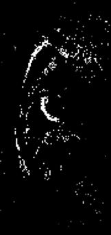
2 = ΓM x N dynamic signal matrix 2 (b) Low rank BLM (r modeling < N) VR x N 1 N 11 U UMMxxr r r r VV r xr N xn 1 1 ΓM x N 11 2 (c) Blind compressive sensing UM x R N R 2 2 r poral bases dictionary dynamic signal matrix (a) ΓM N coefficient coefficient matrix matrix VR x N 1 2 r fewfew temporal temporal bases bases (b) Blind linear model (BLM): r < N sparse dynamic signalcoefficient matrix matrix R many temporal bases (c) Blind compressed sensing (BCS): R > r BCS (R>r) V Rrepresentations Fig. 1. Comparison of blind compressed sensing (BCS)Uand linear model (BLM) of dynamic imaging data: The Casorati M x blind R xn 2 R 1 N and (c). BCS uses 1 form of the dynamic signal Γ is shown in1 (a). The BLM and BCS decompositions of Γ are respectively shown in (b) a large over-complete dictionary, unlike the orthogonal dictionary with few basis functions in BLM; (R > r). Note that the coefficients/ 2 spatial weights in BCS are sparser than that of BLM. The temporal basis functions in the BCS dictionary are representative of specific regions, since they are not constrained to be orthogonal. For example, the 1st, 2nd columns of UM R in BCS correspond respectively to the temporal dynamics of the right and left ventricles in this myocardial perfusion data with motion. We observe that only 4-5 coefficients R per pixel are sufficient to represent the dataset. sparse coefficient matrix temporal bases dictionary dynamic signal matrix rank. The dependence of the degrees of freedom on the number of temporal basis function is the main reason for the tradeoff between accuracy and achievable acceleration in applications with large motion. We introduce a novel dynamic imaging scheme, termed as blind compressive sensing (BCS), to improve the recovery of dynamic imaging datasets with large inter-frame motion. Similar to classical CS schemes [5] [7], the voxel intensity profiles are modeled as a sparse linear combination of basis functions in a dictionary. However, instead of assuming a fixed dictionary, the BCS scheme estimates the dictionary from the undersampled measurements itself. While this approach of estimating the coefficients and dictionary from the data is similar to BLM methods, the main difference is the sparsity assumption on the coefficients. In addition, the dictionary in BCS is much larger and the temporal basis functions are not constrained to be orthogonal (see figure 1). The significantly larger number of basis functions in the BCS dictionary considerably improves the approximation of the dynamic signal, especially for datasets with significant inter-frame motion. The number of degrees of freedom of the BCS scheme is M k +RN 1, where k is the average sparsity of the representation, R is the number of temporal basis functions in the dictionary, and N is the total number of time frames. However, in dynamic MRI, since M >> N the degrees of freedom is dominated by the average sparsity k and not the dictionary size R, for reasonable dictionary sizes. In contrast to BLM, since the degrees of freedom in BCS is not heavily dependent on the number of basis functions, the representation is richer and hence provide an improved trade-off between accuracy and achievable acceleration. An efficient computational algorithm to solve for the sparse coefficients and the dictionary is introduced in this paper. In the BCS representation, the signal matrix Γ is modeled as the product Γ = UV, where U is the sparse coefficient matrix V is the temporal dictionary. The recovery is formulated as a constrained optimization problem, where the criterion is a linear combination of the data consistency term and a sparsity promoting `1 prior on U, subject to a Frobenius norm (energy) constraint on V. We solve for U and V using a majorize-minimize framework. Specifically, we decompose the original optimization problem into three simpler problems. An alternating minimization strategy is used, where we cycle through the minimization of three simpler problems. The comparison of the proposed algorithm with a scheme that alternates between sparse coding and dictionary estimation demonstrates the computational efficiency of the proposed framework; both methods converge to the same minimum, while the proposed scheme is approximately ten times faster. We also observe that the proposed scheme is less sensitive to initial guesses, compared to the extension of the K-SVD scheme [19] to under-sampled dynamic MRI setting. It is seen that the `1 sparsity norm and Frobenius norm dictionary constraint enables the attenuation of insignificant dictionary basis functions, compared with the `0 sparsity norm and column norm dictionary constraint used by most dictionary learning schemes. This implicit model order selection property is important in the under sampled setting since the number of basis functions that can be reliably estimated is dependent on the available data and the signal to noise ratio. The proposed work has some similarities to [20], where a patch dictionary is learned to exploit the correlations between image patches in a static image. The key difference is that the proposed scheme exploits the correlations between voxel time profiles in dynamic imaging rather than redundancies between image patches. The `0 norm sparsity constraints and unit column norm dictionary constraints are assumed in [20]. The adaptation of this formulation to our setting resulted in the learning of noisy basis functions at high acceleration factors. Similar to [21], the setting in [20] permits the reconstructed dataset to deviate from the sparse model. The denoising scheme is well-posed even in this relaxed setting since the authors assume overlapping patches; even if a patch does not have a sparse representation in the dictionary, the pixels in the patch are still constrained by the sparse representations of other patches containing them. Since there is no redundancy in our setting, the adaptation of the above scheme to our setting may also result in alias artifacts. Furthermore, the proposed numerical algorithm is very different from the optimization scheme in [20], where they alternate between a greedy K-SVD dictionary learning algorithm and a reconstruction update step admitting an efficient closed-form solution. We observe that the greedy approach is vulnerable to local minima in the dynamic imaging setting.

3 3 The proposed BCS setup has some key differences with the formulation in [22], where the recovery of several signals measured by the same sensing matrix is addressed; additional constraints on the dictionary were needed to ensure unique reconstruction in this setting. By contrast, we use different sensing matrices (sampling patterns) for different time frames, inspired by prior work in other dynamic MRI problems [5], [8], [13]. Our phase transition experiments show that we obtain good reconstructions without any additional constraints on the dictionary. Since the BCS scheme assumes that only very few basis functions are active at each voxel, this model can be thought of as a locally low-rank representation [17]. However, unlike [17], the BCS scheme does not estimate the basis functions for each neighborhood independently. Since it estimates V from all voxels simultaneously, it is capable of exploiting the correlations between voxels that are well separated in space (non-local correlations). A. Dynamic image acquisition II. DYNAMIC MRI RECONSTRUCTION USING THE BCS MODEL The main goal of the paper is to recover the dynamic dataset γ(x, t) : Z 3 C from its under-sampled Fourier measurements. We represent the dataset as the M N Casorati matrix [10]: γ(x 1, t 1 ).... γ(x 1, t N ) γ(x 2, t 1 ).... γ(x 2, t N ) Γ M N = (1) γ(x M, t 1 ).... γ(x M, t N ) Here, M is the number of voxels in the image and N is the number of image frames in the dataset. The columns of Γ correspond to the voxels of each time frame. We model the measurement process as b i = (S i F T i ) }{{} (Γ) + n i ; i = 1,..., N; (2) A i where, b i and n i are respectively the measurement and noise vectors at the i th time instants. T i is an operator that extracts the i th column of Γ, which corresponds to the image at t i. F is the 2 dimensional Fourier transform and S i is the sampling operator that extracts the Fourier samples on the k-space trajectory corresponding to the i th time frame. We consider different sampling trajectories for different time frames to improve the diversity. B. The BCS representation We model Γ as the product of a sparse coefficient matrix U M R and a matrix V R N, which is a dictionary of temporal basis functions: γ(x 1, t 1 ).... γ(x 1, t N ) u 1 (x 1 ).. u R (x 1 ) γ(x 2, t 1 ).... γ(x 2, t N ) u 1 (x 2 ).. u R (x 2 ) v 1 (t 1 ).. v 1 (t N ) =.... v 2 (t 1 ).. v 2 (t N ) (3) v γ(x M, t 1 ).... γ(x M, t N ) u 1 (x M ).. u R (x M ) R (t 1 ).. v R (t N ) }{{}}{{}}{{} V R N Γ M N U M R Here, R is the total number of basis functions in the dictionary. The model in (3) can also be expressed as the partially separable function (PSF) model [10], [15]: R γ(x, t) = u i (x) v i (t), (4) Here, u i (x) corresponds to the i th column of U and is termed as the i th spatial weight. Similarly, v i (t) corresponds to the i th row of V and is the i th temporal basis function. The main difference with the traditional PSF setting is that the rows of U are constrained to be sparse, which imply that there are very few non-zero entries; this also suggests that few of the temporal basis functions are sufficient to model the temporal profile at any specified voxel. The over-complete dictionary of basis functions are estimated from the data itself and are not necessarily orthogonal. In figure 1, we demonstrate the differences between BLM (low-rank) and BCS representations of a cardiac perfusion MRI data set with motion. Note that the sparsity constraint encourages the formation of voxel groups that share similar temporal profiles. Since many more basis functions are present in the dictionary, the representation is richer than the BLM model. The sparsity assumption ensures that the richness of the model is not translated to increased degrees of freedom. The sparsity assumption also enables the suppression of noise and blurring artifacts, thus resulting in sharper reconstructions. The degrees of freedom associated with BCS is approximately Mk + RN 1, where k is the average sparsity of the coefficients and R is the number of basis functions in the dictionary. Since M >> N, the degrees of freedom in the BCS

4 4 representation is dominated by the average sparsity (k) and not the size of the dictionary (R), for realistic dictionary sizes. Since the overhead in learning the dictionary is low, it is much better to learn the dictionary from the under-sampled data rather than using a sub-optimal dictionary. Hence, we expect this scheme to provide superior results than classical compressive sensing schemes that use fixed dictionaries. C. The objective function We now address the recovery of the signal matrix Γ, assuming the BCS model specified by (3). Similar to classical compressive sensing schemes, we replace the sparsity constraint by an l 1 penalty. We pose the simultaneous estimation of U and V from the measurements as the constrained optimization problem: [ N ] {Û, ˆV} = arg min A i (UV) b i λ U l1 ; such that V 2 F c. (5) U,V The first term in the objective function (5) ensures data consistency. The second term is the sparsity promoting l 1 norm on the entries of U defined as the absolute sum of its matrix entries: U: U l1 = M R j=1 u(i, j). λ is the regularization parameter, and c is a constant that is specified apriori. The Frobenius norm constraint on V is imposed to make the problem well posed; if this constraint is not used, the optimization scheme can end up with coefficients U that are arbitrarily small in magnitude. While other constraints (e.g. unit norm constraints on rows) can also be used to make the problem well-posed, the Frobenius norm constraint along with the l 1 sparsity penalty encourages a ranking of temporal basis functions. Specifically, important basis functions are assigned larger amplitudes, while un-important basis functions are allowed to decay to small amplitudes. We observe that the specific choice of c is not very important; if c is changed, the regularization parameter λ also has to be changed to yield similar results. D. The optimization algorithm The Lagrangian of the constrained optimization problem in (5) is specified by: [ N ] L(U, V, η) = A i (UV) b i λ (U) l1 + η ( V 2 F c ) ; η 0 (6) where η is the Lagrange multiplier (b) (ζ) 0.12 reconstruction error Proposed BCS: Random 1 Proposed BCS: Random 2 Proposed BCS: DCT Alternate BCS: Random 1 Alternate BCS: Random 2 Alternate BCS: DCT Greedy BCS: Random 1 Greedy BCS: Random 2 Greedy BCS: DCT Direct IFFT reconstruction time (minutes) (a) (c) (d) (b) Direct IFFT (c) Greedy BCS (d) Proposed BCS ζ =0.15 ζ = ζ = Fig. 2. Comparison of different BCS schemes: In (a), we show the reconstruction error vs reconstruction time for the proposed BCS, alternate BCS, and the greedy BCS schemes. The free parameters of all the schemes were optimized to yield the lowest possible errors, while the dictionary sizes of all methods were fixed to 45 atoms. We plot the reconstruction error as a function of the CPU run time for the different schemes with different dictionary initializations. The proposed BCS and alternating BCS scheme converged to the same solution irrespective of the initialization. However, the proposed scheme is observed to be considerably faster; note that the alternating scheme takes around ten times more time to converge. It is also seen that the greedy BCS scheme converged to different solutions with different initializations, indicating the dependence of these schemes on local minima.

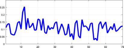
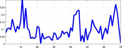
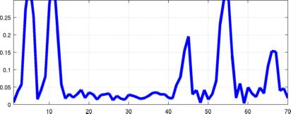
5 5 Since the `1 penalty on the coefficient matrix is a non differentiable function, we approximate it by the differentiable Huber ui (x) {i = 1 to 15} vi (t) ui (x) {i = 16 to 30} vi (t) (a) Proposed BCS ui (x) {i = 1 to 15} vi (t) ui (x) {i = 16 to 30} vi (t) (b) Greedy BCS Model coefficients and dictionary bases. We show few of the estimated spatial coefficients ui (x) and its corresponding temporal bases vi (t) from 7.5 fold undersampled myocardial perfusion MRI data (data in Fig. 2). (a) corresponds to the estimates using the proposed BCS scheme, while (b) is estimated using the greedy BCS scheme. For consistent visualization, we sort the product entries ui (x)vi (t) according to their `2 norm, and show the first 30 sorted terms. Note that the BCS basis functions are drastically different from exponential basis functions in the Fourier dictionary; they represent temporal characteristics specific to the dataset. It can also be seen that the energy of the basis functions in (a) varies considerably, depending on their relative importance. Since we rely on the `1 sparsity norm and Frobenius norm dictionary constraint, the representation will adjust the scaling of the dictionary basis functions vi (t) such that the kuk`1 is minimized. Specifically, the `1 minimization optimization will ensure that basis functions used more frequently are assigned higher energies, while the less significant basis functions are assigned lower energy (see v25 (t) to v30 (t)), hence providing an implicit model order selection. By contrast, the formulation of the greedy BCS scheme involves the setting of `0 sparsity norm and column norm dictionary constraint; the penalty is only dependent on the sparsity of U. Unlike the proposed scheme, this does not provide an implicit model order selection, resulting in the preservation of noisy basis functions, whose coefficients capture the alias artifacts in the data. This explains the higher errors in the greedy BCS reconstructions in Fig. 2. Fig. 3.

6 6 Reconstruction error : (ζ) Reconstruction error: (ζ) Blind CS Blind linear model average no. of non zero model coefficients Blind CS Blind linear model λ no. of bases in the model no. of bases in the model (a) (b) (c) Fig. 4. Blind CS model dependence on the regularization parameter and the dictionary size: (a) shows the reconstruction error (ζ) as a function of different λ in the BCS model. (b) and (c) respectively show the reconstruction error (ζ) and the average number of non zero model coefficients of the BCS and the BLM schemes as a function of the number of bases in the respective models. As depicted in (a), we optimize our choice of λ such that the error between the fully sampled data and the reconstruction is minimal. From (b), we observe that the BCS reconstruction error reduces with the dictionary size and hits a plateau after a size of 20 basis functions. This is in sharp contrast with the BLM scheme where the reconstructions errors increase when the basis functions are increased. The average number of BCS model coefficients unlike the BLM has a non-linear relation with the dictionary size reaching saturation to a number of The plots in (b) and (c) depict that the BCS scheme is insensitive to dictionary size as long as a reasonable size (atleast 20 in this case) is chosen. We chose a dictionary size of 45 bases in the experiments considered in this paper. induced penalty which smooths the l 1 penalty. ϕ β (U) = M j=1 where, u i,j are the entries of U and ψ β (u) is defined as: { x 1/2β if x 1 β ψ β (x) = β x 2 /2 else. R ψ β (u i,j ), (7) The Lagrangian function obtained by replacing the l 1 penalty in (6) by ϕ β is: [ N ] D β (U, V, η) = A i (UV) b i λ ϕ β (U) + η ( V 2 F c ) ; η 0 (9) Note that ϕ β (U) is parametrized by the single parameter β. When β, the Huber induced norm is equivalent to the original l 1 penalty. Other ways to smooth the l 1 norm have been proposed (eg: [23]). We observe that the algorithm has slow convergence if we solve for (5) with β. We use a continuation strategy to improve the convergence speed. Note that the Huber norm simplifies to the Frobenius norm when β = 0. This formulation (ignoring the constant c and optimization with respect to η) is similar to the one considered in [24]; according to the [24, Lemma 5], the solution of (9) is equivalent to the minimum nuclear norm solution. Here, we assume that the size of the dictionary R is greater than the rank of Γ, which holds in most cases of practical interest. Thus, the problem converges to the well-defined nuclear norm solution when β = 0. Our earlier experiments show that the minimum nuclear norm solution already provides reasonable estimates with reduced aliasing [13]. Thus, the cost function is less vulnerable to local minimum when β is small. Hence, we propose a continuation strategy, where β is initialized to zero and is gradually increased to a large value. By slowly increasing β from zero, we expect to gradually truncate the small coefficients of U, while re-learning the dictionary. Our experiments show that this approach considerably improves the convergence rate and avoids local minima issues. We rely on the majorize-minimize framework to realize a fast algorithm. We start by majorizing the Huber norm in (9) as 2 [25]: ϕ β (U) = min L β 2 U L 2 F + L l1, (10) 2 Note that the right hand side of (10) is only guaranteed to majorize the Huber penalty ϕ β (U); it does not majorize the l 1 norm of U; (as from (8) that ψ β (x) is lower than the l 1 penalty by 1/2β when x > 1/β. Similarly ψ β < x /2 when x < 1/β). This majorization in (10) later enables us to exploit simple shrinkage strategies that exist for the l 1 norm; if the l 1 penalty were used instead of the Huber penalty, it would have resulted in more complex expressions than in (16). For additional details, we refer the interested reader to [25]. (8)

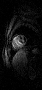
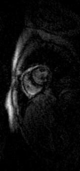
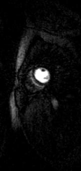
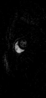
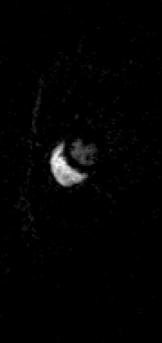
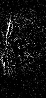
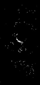
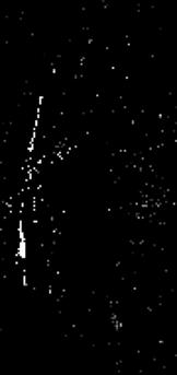
7 7 Γ 1 Γ 2 Γ 3 Γ 10 Fig. 5. The numerical phantoms Γ j, which are used in the simulation study in figure 6. Here j is the number of non zero coefficients (sparsity levels) at each pixel. The top and bottom rows respectively show one spatial frame and the image time profile through the dotted white line. Note that the sparse decomposition provides considerable temporal detail even for a sparsity of one. This is possible since different temporal basis functions are active at each pixel. where L is an auxiliary variable. Substituting (10) in (9), we obtain the following modified Lagrange function, which is a function of four variables U, V, L and η: D(U, V, L, η) = N [ Ai (UV) b i 2 ] ( 2 + η V 2 F c ) [ + λ L l1 + β ] 2 U L 2 F ; (11) The above criterion is dependent on U, V, L, and η and hence have to be solved for all of these variables. While this formulation may appear more complex than the original BCS scheme (5), this results in a simple algorithm. Specifically, we use an alternating minimization scheme to solve (11). At each step, we solve for a specific variable, assuming the other variables to be fixed; we systematically cycle through these subproblems until convergence. The subproblems are specified below. L n+1 = arg min U n L L β L l 1 ; (12) N [ U n+1 = arg min Ai (UV n ) b i 2 λβ 2] + U 2 U L n ; (13) V n+1 = arg min V We use a steepesct ascent rule to update the Lagrange multiplier at each iteration. N [ Ai (U n+1 V) b i 2 ] ( 2 + ηn V 2 F c ) ; (14) η n+1 = ( η n + V n+1 2 F c ) +, (15) where + represents the operator defined as (τ) + = max{0, τ}, which is used to ensure the positivity constraint on η (see (9)). Each of the sub-problems are relatively simple and can be solved efficiently, either using analytical schemes or simple optimization strategies. Specifically, (12) can be solved analytically as: L n+1 = U n U n ( U n 1 β ) ; (16) + Since the problems in (13) and (14) are quadratic, we solve it using conjugate gradient (CG) algorithms. Once V 2 F c, we see that η stabilizes. Hence, we expect (14) to converge quickly. In contrast, the condition number of the U sub-problem is dependent on β. Hence, the convergence of the algorithm will be slow at high values of β. In addition, the algorithm may converge to a local minimum if it is initialized directly with a large value of β. We use the above mentioned continuation approach to solve for simpler problems initially and progressively increase the complexity. Specifically, starting with an initialization of V, the algorithm iterates between (12) and (15) in an inner loop, while progressively updating β starting with a small value in an outer loop. The inner loop is terminated when the cost in (6) stagnates. The outer loop is terminated when a large enough β is achieved. We define convergence as when the cost in (6) in the outer loop stagnates to a threshold of In general, with our experiments on dynamic MRI data, we observed convergence when the final value of β is approximately to times larger than the initial value of β.

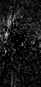
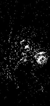
8 8 III. EXPERIMENTAL EVALUATION We describe in sections (III. A-B) the algorithmic considerations of the proposed blind CS framework. We then perform phase transition experiments using numerical phantoms to empirically demonstrate the uniqueness of the blind CS framework (section III.C). We finally compare the reconstructions of blind CS against existing low rank and compressed sensing schemes using invivo Cartesian and radial free breathing myocardial perfusion MRI datasets (section III.D). A. Comparison of different BCS schemes In this section, we compare the performance of the proposed scheme with two other potential BCS implementations. Specifically, we focus on the rate of convergence and the sensitivity to initial guesses of the following schemes: Proposed BCS: The proposed BCS formulation specified by (5) solved by optimizing U and V using the proposed majorize-minimize algorithm; the algorithm cycles through steps specified by (12)-(15). Alternating BCS: The proposed BCS formulation specified by (5) solved by alternatively optimizing for the sparse coefficients U and the dictionary V. Specifically, the sparse coding step (solving for U, assuming a fixed V) is performed using the state of the art augmented Lagrangian optimization algorithm [26]. The dictionary learning sub-problem solves for V, assuming U to be fixed. This is solved by iterating between a quadratic subproblem in V (solved by a conjugate gradient algorithm), and a steepest ascent update rule for η (similar to (15)). The update of η ensures the Frobenius norm constraint on V is satisfied at the end of the V sub-problem. Both of the sparse coding and dictionary learning steps are iterated until convergence. Greedy BCS: We adapt the extension of the K-SVD scheme that was used for patch based 2D image recovery [20] to our setting of dynamic imaging. This scheme models the rows of Γ in the synthesis dictionary with temporal basis functions # of radial lines sparsity level: j # of radial lines sparsity level: j # of radial lines sparsity level: j (a) CS exploiting Fourier sparsity (b) Dictionary unaware: Blind CS (c) Dictionary aware # of radial lines sparsity level: j # of radial lines sparsity level: j # of radial lines sparsity level: j (d) CS exploiting Fourier sparsity (e) Dictionary unaware: Blind CS (f) Dictionary aware Fig. 6. Phase transition behavior of various reconstruction schemes: Top row: Normalized reconstruction error ζ is shown at different acceleration factors (or equivalently different number of radial rays in each frame) for different values of j. Bottom row: ζ thresholded at 1 percent error; black represents 100 percent recovery. We study the ability of the algorithms to reliably recover each of the data sets Γ j from different number of radial samples in kspace. The Γ j, shown in Fig. 5 are the j sparse approximations of a myocardial perfusion MRI dataset with motion. As expected, the number of lines required to recover the dataset increases with the sparsity. The blind CS scheme outperformed the compressed sensing scheme considerably. The learned dictionary aware scheme yielded the best recovery rates. However due to a small over head in estimating the dictionary, the dictionary unaware (blind CS) scheme was only marginally worse than the dictionary aware scheme.

9 9 a b c Sampling mask for one frame Display scale Image Error i. Fully sampled ii. Direct IFFT ζ ROI = HFEN = iii. Low rank: Schatten p-norm regularized ζ ROI = HFEN = iv. CS - Fourier sparsity ζ ROI = HFEN = v. Blind CS ζ ROI = HFEN = a a a a (a - b) Few spatial frames (c) Image time profile (d - e) Error images (f) Error time profile b c b c d e f b c d e f b c d e f d e f Fig. 7. Comparison of the proposed scheme with different methods on a retrospectively downsampled Cartesian myocardial perfusion data set with motion at 7.5 fold acceleration: A radial trajectory is used for downsampling. The trajectory for one frame is shown in (i). The trajectory is rotated by random shifts in each time frame. Reconstructions using different algorithms, along with the fully sampled data are shown in (i) to (v). (a-b), (c), (d-e), (f) respectively show few spatial frames, image time profile, corresponding error images, error in image time profile. The image time profile in (c) is through the dotted line in (i.b). The ripples in (i.c) correspond to the motion due to inconsistent gating and/or breathing. The location of the spatial frames along time is marked by the dotted lines in (i.c). We observe the BCS scheme to be robust to spatio-temporal blurring, compared to the low rank model; eg: see the white arrows, where the details of the papillary muscles are blurred in the Schatten p-norm reconstruction while maintained well with BCS. This is depicted in the error images as well, where BCS has diffused errors, while the low rank scheme (iii) have structured errors corresponding to the anatomy of the heart. The BCS scheme was also robust to the compromises observed with the CS scheme ; the latter was sensitive to breathing motion as depicted by the arrows in iv. (as in (4)). Specifically, it solves the following optimization problem: {ˆΓ, Û, ˆV} = arg min Γ,U,V UV 2 2; such that N A i (Γ) b i 2 2 < σ n, u k 0 j; k = 1,..., M, v q 2 2 = 1; q = 1,..., R; (17) where σ n is the standard deviation of the measurement noise. Here the l 0 norm is used to impose the sparsity constraints on the rows (indexed by k) of U. The number of nonzero coefficients (or the sparsity level) of each row of U is given by j. The unit column norm constraints are used on the elements of the dictionary to ensure well posedness (avoid scaling ambiguity). Starting with an initial estimate of the image data given by the zero filled inverse Fourier reconstruction Γ init,

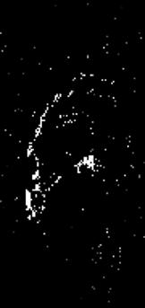
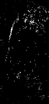
10 10 a spatial frame image time series Sampling for one frame Error images (x10 scaled) (a) fully sampled (b) Low rank ζ = HFEN = (c) CS- Fourier sparsity ζ = HFEN = (d) BCS ζ = HFEN = Fig. 8. Comparisons of the different reconstructions schemes on a brain perfusion MRI dataset. The fully sampled data in (a) is retrospectively undersampled at a high acceleration of The radial sampling mask for one frame is shown in (a), subsequent frames had the mask rotated by random angles. We show a spatial frame, the image time series, and the corresponding error images for all the reconstruction schemes. Note from (b,c), the low rank and CS schemes have artifacts in the form of spatiotemporal blur; the various fine features are blurred (see arrows). In contrast, the BCS scheme had crisper features, and superior spatiotemporal fidelity. The reconstruction error and the HFEN error numbers were also considerably less with the BCS scheme. a b c c Acquired (72 rays) Golden ratio under-sampling (24 rays) Display scale Image Error i. Reference ii. Low rank: Schatten p-norm regularized ζ ROI = HFEN = iii. CS-Fourier sparsity ζ ROI = HFEN = iv. Blind CS ζ ROI = HFEN = (a - b) Few spatial frames (c) Image time profile (d - e) Error images (f) Error time profile a b c b c d e d f e f a b b c c d e d f e f a b b c c d e f Fig. 9. Comparisons of different reconstruction schemes on a stress myocardial perfusion MRI dataset with breathing motion: Retrospective sampling was considered by picking 24 radial rays/frame from the acquired 72 ray data; the rays closest to the golden ratio pattern was chosen. Few spatial frames, the corresponding image time profile, error frames, and error in image time profile are shown for all the schemes. We specifically observe loss of important borders and temporal blur with the low rank and CS schemes while the blind CS reconstructions have crisper borders and better temporal fidelity. Also note from the columns d,e,f that the errors in the BCS scheme are less concentrated at the edges, compared to the other methods. This indicates that the edge details and temporal dynamics are better preserved in the BCS reconstructions. the BCS scheme in this setting iterates between a denoising/dealiasing step to update U, V, and an image reconstruction step to update Γ. The denoising step involves dictionary learning and sparse coding with l 0 minimization. It utilizes

11 11 the K-SVD algorithm [19] which takes a greedy approach to update U and V. We implemented the K-SVD algorithm based on the codes available at the authors webpage [27]. The K-SVD implementation available online was modified to produce complex dictionaries. For sparse coding, we used the orthogonal matching pursuit algorithm (OMP). We used the approximation error threshold along with the sparsity threshold (upper bound on j) in OMP. The approximation error threshold was set to Our implementation also considered the pruning step described in [19], [21] to minimize local minima effects. Specifically, if similar basis functions were learnt, one of them was replaced with the voxel time profile that was least represented. In addition, if a basis function was not being used enough, it was replaced with the voxel time profile that was least represented. Other empirical heuristics such as varying the approximation error threshold in the OMP algorithm during the different iteration (alteration) steps may also be considered in the greedy BCS scheme. In this work, we restrict ourselves to a fixed error threshold of 10 6 due to the difficulty of tuning for an optimal set of different error threshold values for different alteration steps. In Fig. 2, we aim to recover a myocardial perfusion MRI dataset with considerable interframe motion (N x N y N t = ) from its undersampled k t measurements using the above three BCS schemes. We considered a noiseless simulation in this experiment for all the three BCS schemes. While resampling, we used a radial trajectory with 12 uniformly spaced rays within a frame with subsequent random rotations across frames to achieve incoherency. This corresponded to an acceleration of 7.5 fold. We used 45 basis functions in the dictionary. We compare the performance of the different BCS algorithms with different initializations of the dictionary V. Specifically, we used dictionaries with random entries, and a dictionary with the discrete cosine transform (DCT) bases. To ensure fair comparisons, we optimized the parameters of all the three schemes: (i.e, regularization parameter λ in the proposed and alternating BCS schemes, as well as the sparsity level j in the greedy BCS scheme). These were chosen such that the normalized error between the reconstruction and the fully sampled data was minimal. A sparsity level of j = 3 was found to be optimal for the greedy BCS scheme. Further, in the greedy BCS scheme, after the first iteration, we initialized the K-SVD algorithm with the dictionary obtained from the previous iteration. We used the same stopping criterion in both the proposed and alternate BCS schemes: the iterations were terminated when the cost in (6) stagnated to a threshold of All the algorithms were run on a linux work station with a 4 core Intel Xeon processor and 24 GB RAM. From Fig. 2, we observe both the proposed and alternate BCS schemes to be robust to the choice of initial guess of the dictionary. They converged to almost the same solution with different initial guesses. However, the proposed BCS scheme converged to the solution significantly faster (atleast by a factor of 10 fold) compared to the alternate BCS scheme. From Fig. 2, we observe the number of iterations for both the proposed and the alternate BCS schemes to be similar. However, since the alternate BCS scheme solves for the sparse l 1 minimization problem fully during each iteration, it is more expensive than the proposed BCS scheme. On an average, an iteration of the alternate BCS scheme was 10 slower than an iteration of the proposed BCS scheme. From Fig. 2, we note the greedy BCS scheme to converge to different solutions for different initial guesses. Additionally, as noted in Fig. 2 c.d, the reconstructions with the proposed BCS scheme were better than the reconstructions with the greedy BCS scheme. Although the temporal dynamics were faithfully captured in the greedy BCS reconstructions, it suffered from noisy artifacts. This was due to modeling with noisy basis functions, which were learned by the algorithm from under sampled data (see Fig. 3). Note that this scheme uses the unit column norm constraints which has all the basis functions are ranked equally. In contrast, since the proposed scheme uses the l 1 sparsity penalty and the Frobenius norm dictionary constraint, the energy of the learned bases functions varied considerably (see Fig. 3). With the proposed scheme, the l 1 minimization optimization ensures that the important basis functions (basis functions that are shared by several voxels) will have a higher energy. Similarly, the un-important noise-like basis functions that play active roles in fewer voxels will be attenuated, since the corresponding increase in U l1 is small. Thus, the l 1 penalty-frobenius norm combination results in a model order selection, which is more desirable than the l 0 penalty-column norm combination. This choice is especially beneficial in the undersampled case since the number of basis functions that can be reliably recovered is dependent on the number of measurements and the signal to noise ratio. B. Choice of parameters The performance of the blind CS scheme depends on the choice of two parameters: regularization parameter λ and the number of bases in the dictionary R. Eventhough the criterion in (5) depends on c, varying it results in a renormalization of the dictionary elements and hence changing the value of λ. We set the value of c as 800 for both the numerical and invivo experiments. We now discuss the behavior of the blind CS model with respect to changes in λ and R. 1) Dependence on λ: We observe that if a low λ is used, the model coefficient matrix U is less sparse. This results in representing each voxel profile using many temporal basis functions. Since the number of degrees of freedom on the scheme depends on the number of sparse coefficients, this approach often results in residual aliasing in datasets with large motion. In contrast, heavy regularization results in modeling the entire dynamic variations in the dataset using very few temporal basis functions; this often results in temporal blurring and loss of temporal detail. In the experiments in this paper, we have access to the fully sampled ground truth data. As depicted in figure 4 (a), we choose the optimal λ such that the error between the

12 12 reconstructions and the fully sampled ground truth data, specified by ( Γrecon Γ orig 2 ) F ζ = Γ orig 2. (18) F is minimized. Furthermore, in invivo experiments with myocardial perfusion MRI datasets, we optimize λ by evaluating the reconstruction error only in a field of view that contained regions of the heart (ζ ROI, ROI: region of interest), specified by ( Γrecon,ROI Γ orig,roi 2 ) F ζ ROI = Γ orig,roi 2. (19) F This metric is motivated by recent findings in [28], and by our own experience in determining a quantitative metric that best describes the accuracy in reproducing the perfusion dynamics in different regions of the heart, and the visual quality in terms of minimizing visual artifacts, and preserving crispness of borders of heart. We realize that the above approach of choosing the regularization parameter is not feasible in practical applications, where the fully sampled reference data is not available. In these cases, one can rely on simply heuristics such as the L-curve strategy [29], or more sophisticated approaches for choosing the regularization parameters [30], [31]. The discussion of these approaches in this context are beyond the scope of this paper. 2) Dependence on the dictionary size: In figure 4.b & 4.c, we study the behavior of the BCS model as the number of basis functions in the model increase. We perform BCS reconstructions using dictionary sizes ranging from 5 to 100 temporal bases. The plot the reconstruction errors and the average number of non-zero model coefficients 3 as a function of the number of basis functions are shown in figures 4.b & 4.c, respectively. We observe that the BCS reconstructions are insensitive to the dictionary size beyond basis functions. We attribute the insensitivity to number of basis functions to the combination of the l 1 sparsity norm and the Frobenius norm constraint on the dictionary (see Fig. 3). Note that the number of basis functions that can be reliably estimated from under sampled data is limited by the number of measurements and the signal to noise ratio, unlike the classical dictionary learning setting where extensive training data is available. As discussed earlier (section III.A), the l 1 sparsity norm and the Frobenius norm dictionary constraint allows the energy of the basis functions to be considerably different. Hence, the optimization scheme ranks the basis functions in terms of their energy, allowing the insignificant basis functions (which models the alias artifacts and noise) to decay to very small amplitudes. Based on these above observations, we fix the BCS dictionary size to 45 basis functions in the rest of the paper. Note that since 45 < 70 = the number of time frames of the data, this is an undercomplete representation. From figure 4 (c), we observe that the average number of non zero model coefficients to be approximately constant ( 4 4.5) for dictionary sizes greater than 20 bases. The BCS model is also compared to the blind linear model (low-rank representation) in figures 4 (b & c). The number of non zero model coefficients in the blind linear model grows linearly with the number of bases. This implies that the temporal bases modeling error artifacts and noise are also learned as the number of basis functions increase. This explains the higher reconstruction errors observed with the blind linear models as the number of basis functions increase beyond a limit. C. Numerical simulations To study the uniqueness of the proposed BCS formulation in (5), we evaluate the phase transition behavior of the algorithm on numerical phantoms. We generate dynamic phantoms with varying sparsity levels by performing dictionary learning on a fully sampled myocardial perfusion MRI dataset with motion (N x N y N t = ); i.e., M = 17100; N = 70. We use the K-SVD algorithm [19] to approximate the fully sampled Casorati matrix Γ M N as a product of a sparse coefficient matrix U j M R, and a learned dictionary Vj R N by solving {Ûj, ˆVj } = arg min U j,v j Γ Uj V j 2 F s.t. u i 0 j; i = 1, 2,.., M, v q 2 = 1; q = 1,..., R; (20) Here, j denotes the number of non zero coefficients in each row of U j. We set the size of the dictionary as R = 45. We construct different dynamic phantoms corresponding to different values of j ranging from (j = 1, 2,..10) as Γ j = U j V j. Few of these phantoms are shown in figure 5. Note that the K-SVD model is somewhat inconsistent with our formulation since it relies on l 0 penalty and uses the unit column norm constraint, compared to the l 1 penalty and Frobenius norm constraint on the dictionary in our setting. We perform experiments to reconstruct the spatio-temporal datasets Γ j from k t measurements that are undersampled at different acceleration factors. Specifically, we employ a radial sampling trajectory with l number of uniformly spaced rays within a frame with subsequent random rotations across time frames; the random rotations ensure incoherent sampling. We 3 Evaluated by performing the average of the number of non-zero coefficients in the rows of the matrix U M R that was thresholded at 1 percent of the maximum value of U.

13 13 consider different number of radial rays ranging from l = 4, 8, 12,.., 56 to simulate undersampling at different acceleration rates. The reconstructions were performed with three different schemes: 1) classical compressed sensing method, where the signal is assumed to be sparse in the temporal Fourier domain (CS) [5]. 2) the proposed blind CS method, where the sparse coefficients and the dictionary are estimated from the measurements. 3) dictionary aware CS: this approach is similar to 1, except that the dictionary V j is assumed to be known. This case is included as an upper-limit for acheivable acceleration. The performance of the above schemes were compared by evaluating the normalized reconstruction error metric ζ (18). All the above reconstruction schemes were optimized for their best performance by tuning the regularization parameters such that ζ was minimal. The phase transition plots of the reconstruction schemes are shown in figure 6. We observe that the CS scheme using Fourier dictionary result in poor recovery rates in comparison to the other schemes. This is expected since the myocardial perfusion data is not sparse in the Fourier basis. As expected, the dictionary aware case (the exact dictionary in which the signal is sparse is pre-specified) provides the best results. However, we observe that the performance of the BCS scheme is only marginally worse than the dictionary aware scheme. As explained before, most of the degrees of freedom in the BCS representation is associated with the sparse coefficients. By contrast, the number of free parameters associated with the dictionary is comparatively far smaller since the number of voxels is far greater than the number of time frames. This clearly shows that the overhead in additionally estimating the dictionary is minimal in the dynamic imaging scenario. This property makes the proposed scheme readily applicable and very useful in dynamic imaging applications (e.g. myocardial perfusion, free breathing cine), where the signal is not sparse in pre-specified dictionaries. D. Experiments on invivo datasets 1) Data acquisition and undersampling: We evaluate the performance of the BCS scheme by performing retrospective undersampling experiments on contrast enhanced dynamic MRI data. We consider one brain perfusion MRI dataset acquired using Cartesian sampling, and two free breathing myocardial perfusion MRI datasets that were acquired using Cartesian sampling, and radial sampling respectively. The myocardial perfusion MRI datasets were obtained from subjects scanned on a Siemens 3T MRI at the University of Utah in accordance to the institute s review board. The Cartesian dataset was acquired under rest conditions after a Gd bolus of 0.02 mmol/kg. The radial dataset was acquired under stress conditions where 0.03 mmol/kg of Gd contrast agent was injected after 3 minutes of adenosine infusion. The Cartesian dataset (phase frequency encodes time = ) was acquired using a saturation recovery FLASH sequence (3 slices, TR/TE =2.5/1.5 ms, sat. recovery time = 100 ms). The motion in the data was due to improper gating and/or breathing; (see the ripples in the time profile in figure 7(c)). The radial data was acquired with a perfusion radial FLASH saturation recovery sequence (TR/TE 2.5/1.3 ms ). 72 radial rays equally spaced over π radians and with 256 samples per ray were acquired for a given time frame. The rays in successive frames were rotated by a uniform angle of π/288 radians, which corresponds to a period of 4 across time. The acquired radial data corresponds to an acceleration factor of 3 compared to Nyquist. Since this dataset is slightly under sampled, we use a spatio-temporal total variation (TV) constrained reconstruction algorithm to generate the reference data in this case. We observe that this approach is capable of resolving the slight residual aliasing in the acquired data. The single slice brain perfusion MRI dataset was obtained from a multi slice 2D dynamic contrast enhanced (DCE) patient scan at the University of Rochester. The patient had regions of tumor identified in the DCE study. The data corresponded to 60 time frames separated by TR=2sec; the matrix size was Retrospective downsampling experiments were done using two different sampling schemes respectively for the Cartesian and radial acquisitions. Specifically, the Cartesian datasets were resampled using a radial trajectory with 12 uniformly spaced rays within a frame with subsequent random rotations across frames to achieve incoherency. This corresponds to a net acceleration level of 7.5 in the cardiac data, and in the brain data. Retrospective undersampling of the cardiac radial data was done by considering 24 rays from the acquired 72 ray dataset. These rays were chosen such that they were approximately separated by the golden angle distance (π/1.818). The golden angle distribution ensured incoherent k-t sampling. The acquisition using 24 rays corresponds to an acceleration of 10.6 fold when compared to Nyquist. This acceleration can be capitalized to improve many factors in the scan (eg: increase the number of slices, improve the spatial resolution, improve quality in short duration scans such as systolic or ungated imaging). 2) Evaluation of blind CS against other reconstruction schemes: We compare the BCS algorithm against the following schemes: low rank promoting reconstruction using Schatten p-norm (Sp-N) (p = 0.1) minimization [13]. compressed sensing (CS) exploiting temporal Fourier sparsity [5] We compared different low-rank methods including two step low rank reconstruction [10], nuclear norm minimization [13], incremented rank power factorization (IRPF) [12], and observed that the Schatten p-norm minimization scheme provides comparable, or even better, results in most cases that we considered [32]. Hence we chose the Schatten p-norm reconstruction scheme in our comparisons. For a quantitative comparison amongst all the methods, we use the normalized reconstruction