GPU-Accelerated Real-Time Stereo Matching. Master s thesis in Computer Science algorithms, languages and logic PETER HILLERSTRÖM

Transcription

1 GPU-Accelerated Real-Time Stereo Matching Master s thesis in Computer Science algorithms, languages and logic PETER HILLERSTRÖM Department of Computer Science and Engineering CHALMERS UNIVERSITY OF TECHNOLOGY UNIVERSITY OF GOTHENBURG Gothenburg, Sweden 2017

2

3 Master s thesis 2017 GPU-Accelerated Real-Time Stereo Matching PETER HILLERSTRÖM Department of Computer Science and Engineering Chalmers University of Technology University of Gothenburg Gothenburg, Sweden 2017

4 GPU-Accelerated Real-Time Stereo Matching PETER HILLERSTRÖM PETER HILLERSTRÖM, Supervisor: Erik Sintorn, Department of Computer Science and Engineering Advisor: Erik Landolsi, Visionists AB Examiner: Ulf Assarsson, Department of Computer Science and Engineering Master s Thesis 2017 Department of Computer Science and Engineering Chalmers University of Technology and University of Gothenburg SE Gothenburg Telephone Cover: In the upper left quadrant, the Adirondack stereo images from the Middlebury 2014 dataset and a disparity map generated by our algorithm. In the other quadrants, a simple 3D visualization of the scene portrayed by the images, made using the disparity map. Typeset in L A TEX Gothenburg, Sweden 2017 iv

5 GPU-Accelerated Real-Time Stereo Matching PETER HILLERSTRÖM Department of Computer Science and Engineering Chalmers University of Technology and University of Gothenburg Abstract A problem in the field of computer vision is the correspondence problem, the problem of finding pixels which correspond to each other in different images. A stereo matching algorithm is used to solve this kind of problem, and typically produces a disparity map, or a depth map. Current approaches are often too slow to be used in real-time, leading to the question of which algorithm is best for such purposes. This thesis explores which approach to stereo matching is most appropriate for real-time purposes. In addition, it is also explored what optimizations and approximations can be applied in order to improve performance. This was accomplished by implementing an Adaptive Support Weights based stereo matching algorithm in CUDA, and exploring various approximations and performance optimizations related to it. It is shown that Adaptive Support Weights is a good method for real-time use. This thesis most significant contribution is the performance optimizations presented, which significantly improve upon the performance of the algorithm compared to previous work. Keywords: Stereo vision, stereo matching, gpu, cuda, optimization, real-time, adaptive support weights v

6

7 Acknowledgements First off, I would like to thank Erik Landolsi at Visionists for this opportunity. Also, thanks to him and the others at Visionists for making me feel welcome during this time. Thanks also goes to my supervisor Erik Sintorn, who spent a lot of his valuable time discussing intricate details about this work. Thanks to the entire Computer Graphics Research Group for putting up with me when I have visited. This work was done at Visionists AB and supported by OP Teknik AB. Peter Hillerström, Gothenburg, June 2017 vii

8

9 Contents 1 Introduction Motivation Problem Definition Previous Work Evaluation and Comparison Semi-Global Matching Neural Networks Adaptive Support Weights Matching Cost Functions Theory Stereo Matching Epipolar Geometry and Rectification Structure of a Stereo Matching Algorithm Cost Computation Disparity Selection Adaptive Support Weights Support Weights Two-Pass Approximation Refinement Consistency Check Census Transform GPU Programming CUDA Thread Blocks Shared Memory Implementation Method Structure Aggregation Phase Refinement Phase Implementation Details Color Difference in Support Weight Calculation Window Size ix

10 Contents Memory Usage Census Window Size Performance Optimization Simplifying Support Weight Expressions CUDA Video SIMD Instructions Rolling Threads Results Testing Environment Datasets and Error Metrics Hardware Default Configuration and Constants Quality Aggregation Phase Quality Refinement Phase Quality Overall Quality Performance Aggregation Phase Refinement Phase Memory Usage Conclusion Discussion Results Future Work Ethical Considerations Conclusion Bibliography 55 x

11 1 Introduction Humans, and other two-eyed animals, are capable of perceiving depth through a process known as stereopsis, or stereo vision. Essentially, two different images are compared, and conclusions are drawn from the differences. If an object is at the same position in both views, it is far away. If the object is horizontally offset in the views, it is close to the viewer. In 1960, Julesz [1] showed that humans are capable of seeing 3D patterns hidden in two images seemingly only containing noise. The images consisted of a large number of dots, some which corresponded to the hidden shape, some which were just noise. The implication of this is that humans are inherently capable of pairing together dots which correspond to the same object from two horizontally offset images. Thus, the problem of stereo correspondence was introduced. The problem of stereo correspondence consists of finding which pixels correspond to which in two horizontally offset images. By solving it, the pixelwise depth to the objects shown in the images can be acquired. Finding the depth for an image is useful for many purposes. For one, it can be used for 3D reconstruction, the process of creating a 3D representation of a real object. Another common use of stereo vision is robotics, where it can for example be used for navigation [2]. A stereo matching method is used to solve the stereo correspondence problem. It is not an easy problem to solve, with many methods having been published throughout the years [3]. It is particularly hard to create accurate methods that are fast enough to be used in real-time. 1.1 Motivation In this section, a problem that requires a fast stereo matching algorithm is described. The problem is related to creating a system to assist drivers of logging trucks to load the truck with logs. A certain type of logging truck has an arm that can be used to pick up logs. Such a logging truck is shown in Figure 1.1. This arm can be controlled from the small 1

12 1. Introduction Figure 1.1: A logging truck with an arm which can be used to pick up logs. cabin in the back of the truck, but also via remote control. It would be beneficial if the driver could load the truck without having to exit the driver s cabin. For one, it could potentially speed up the process of loading logs. But it could also lead to the removal of the arm cabin in future truck models, saving money and resources. The problem is that it is hard to control the arm from the position of the driver s cabin. Specifically, it can be hard to get a good viewpoint of the logs and the arm. A simple solution would be to mount cameras on the truck, and deliver video feeds from them to a screen in the driver s cabin. This leads to the question of whether other systems to assist the driver could be implemented. Specifically, it was suggested to use stereo vision. The depth information retrieved could then either be used for a 3D reconstruction of the scene, or simply to add assisting overlays to the video feeds. Since the arm and logs are moving around, a real-time stereo matching algorithm is necessary. 1.2 Problem Definition In order to select an appropriate solution for the problem described in Section 1.1, it is necessary to perform a study on currently existing state of the art stereo matching algorithms. In particular, algorithms which are fast enough to be used in real-time is of interest. The goal of this thesis is to explore the following questions: What stereo matching algorithm is most suited for real-time use, while still creating high-quality results? What approximations and optimizations can be applied to improve upon existing work? These questions are explored through the implementation of a state of the art stereo matching algorithm. A ranking of many such algorithms is available at the Middle- 2

13 1. Introduction bury Stereo Vision Page 1. At the time of writing, an algorithm by Kowalczuk et al. [4] is the top-ranked one in terms of speed. This algorithm is also the one that was chosen to be implemented and explored in thesis. The motivation for this choice is explained in Section 4.1. A few topics are explicitly excluded from this thesis. The first is the process of rectification, which is briefly explained in Section It is simply assumed that perfectly rectified images will be available for use. The second topic that is excluded is 3D reconstruction. This thesis only covers stereo matching, how the resulting output should be used is not explored. 1 vision.middlebury.edu/stereo/ 3

14 1. Introduction 4

15 2 Previous Work Stereo matching is an active area of research, with new algorithms being published continuously. For this project a fast, yet accurate, method was needed. This chapter summarizes the most relevant approaches to stereo matching. 2.1 Evaluation and Comparison Scharstein and Szeliski [3] have created a taxonomy to compare and evaluate existing stereo matching algorithms. Their taxonomy includes: Matching cost computation: A function used to assign a cost for matching two given pixels. Cost (support) aggregation: The process of aggregating multiple matching costs together to a single cost, mainly used in local algorithms. Disparity computation / optimization: The process of selecting disparity values for each pixel given the previously calculated costs. Disparity refinement: Refinement of a calculated disparity map. They also mention that stereo matching algorithms are often separated into global and local approaches. Local algorithms look at pixels within a local window around the pixel being considered, while global algorithms attempt to minimize a global cost function with smoothness constraints. In addition to the taxonomy, they also created a platform for comparing the performance and quality of stereo matching algorithms. This comparison is hosted at the Middlebury Stereo Vision Page 1, simply referred to as Middlebury from this point on. Middlebury has become a standard benchmark for stereo matching algorithms, with many modern algorithms being hosted there. Middlebury has several ground truth datasets available. A ground truth dataset contains stereo images with known depth for each pixel. The latest dataset at the time of writing is the Middlebury 2014 dataset [5]. 1 vision.middlebury.edu/stereo/ 5

16 2. Previous Work An alternative to Middlebury is the KITTI Vision Benchmark Suite 2. Similarly to Middlebury, they also publish ground truth datasets [6][7]. 2.2 Semi-Global Matching Hirschmuller [8] proposed a method called Semi-Global Matching (SGM ). The main strength of SGM is that it uses a fast approximation of a global cost function. SGM also uses mutual information as the matching cost function, which makes it more robust against images with different illumination. A modified version of SGM is available in OpenCV 3, called StereoSGBM 4. OpenCV is a commonly used open source computer vision library. The inclusion of SGM makes it an easily available stereo matching solution. Some modifications are made to the algorithm in this implementation, among other things the matching cost function is replaced with one introduced by Birchfield and Tomasi [9]. There are several CUDA based implementations of SGM. Examples include Ernst and Hirschmüller [10], Haller and Nedevschi [11], and recently Hernandez-Juarez et al. [12]. 2.3 Neural Networks Žbontar and LeCun [13] introduced a stereo matching method that uses a convolutional neural network to calculate the matching cost. The network was trained on publicly available stereo image datasets with known disparity, including the Middlebury 2014 [5] and KITTI [6] [7] datasets. Two versions of the network were developed, one designed to be fast and one designed to be as accurate as possible. Neural networks are currently used by many of the top-ranking methods on the Middlebury benchmark. Examples of methods that use the matching cost network introduced by Žbontar and LeCun [13] directly include Drouyer et al. [14], Li et al. [15], Zhang et al. [16] (only the extended variant), Kim and Kim [17] and Barron and Poole [18]. In addition, Park and Lee [19] builds upon and improves the network. 2.4 Adaptive Support Weights Adaptive Support Weights (ASW ) is a method introduced by Yoon and Kweon [20]. The method defines support weights for all pixels inside the local window around

17 2. Previous Work a given pixel, for each pixel in both input images. Each support weight represents how similar a neighboring pixel is to the pixel in question. These support weights are then used during cost aggregation to weight the matching cost of similar pixels higher. Wang et al. [21] introduced a two-pass approximation of the original algorithm, to reduce the computational complexity. A local window with dimensions w w is approximated as one w 1 and one 1 w window. The first pass uses the first window to aggregate costs. The second pass aggregates the previously aggregated costs, using the second window, into a final cost. Kowalczuk et al. [4] created an efficient CUDA implementation and added a refinement phase to the algorithm. The refinement phase adds a cost penalty term for selecting disparities that differs from the expected value, given the previously selected disparities in a local window. Disparities are reselected iteratively using the continuously updated cost penalty terms. The implementation by Kowalczuk et al. [4] currently holds the top-spot as the fastest algorithm on Middlebury. At the same time, it is also reported to have almost the same quality as SGM by Hirschmuller [8]. It should however be noted that the quality is reported to be better than the SGM implementation used in OpenCV. 2.5 Matching Cost Functions Many matching cost functions have been proposed for stereo matching. A matching cost function is responsible for calculating a cost for matching two given pixels. Examples of simple functions include squared intensity differences and absolute intensity differences [3] Zabih and Woodfill [22] proposed the rank transform and the census transform. These are both non-parametric local transforms, which means that they rely on the order of pixel s values instead of the values themselves. The rank transform measures local intensity while the census transform summarizes local structure. Hirschmuller and Scharstein [23] has shown that census transform was the most robust matching cost function among the ones they tested in an evaluation of the performance of matching costs functions for images with radiometric differences, e.g. images with different exposure. They also state that census transform performs well also at images without explicit radiometric differences. The reason for this is that some implicit radiometric differences are unavoidable. 7

18 2. Previous Work 8

19 3 Theory This chapter covers the general theory behind stereo matching, the Adaptive Support Weights (ASW ) algorithm, and the census transform matching cost function. In addition, a brief overview of GPU programming using CUDA is provided. 3.1 Stereo Matching Using a calibrated pair of cameras, it is possible to create an image pair showing the same scene from slightly different viewpoints. Using the orientations and positions of the cameras, it is possible to rectify these images so they appear on the same image plane. This sets up the correspondence problem. By finding matching pairs of pixels in both images it is possible to calculate their position in space. A stereo matching algorithm is used to estimate the correspondence between the pixels of these two input images. This section will elaborate on some steps common to most stereo matching algorithms Epipolar Geometry and Rectification Epipolar geometry is the relative geometry between two views. This relative geometry is mainly useful for two reasons; it tells us which pixels need to be considered for matching, and it can be used to reconstruct the scene when the pixel correspondences are known. Figure 3.1 shows an example of epipolar geometry. Knowledge of the epipolar geometry can be used to reduce the search space of a stereo matching algorithm. Without any knowledge of the positions and orientations of the viewpoints, a pixel in the first image could theoretically correspond to any pixel in the other image. If the position and orientation of both views are known, the line from the origin of one view through a given pixel projects to a line on the other view s image plane. This projected line is known as the epipolar line and is shown in Figure 3.1. Hence, only pixels along the epipolar line need to be considered for matching. If the two images are rectified, the epipolar line is simply a row in the other image. 9

20 3. Theory X 0 X 1 X 2 X L X R O L O R Figure 3.1: An example of epipolar geometry. The line, starting from the origin of the left view O L and continuing through the pixel on the image plane X L, is projected onto the right image plane. This projected line is known as the epipolar line, and is shown as a red line in the figure. The images can be considered rectified if the only thing that differs between the views is a horizontal offset. I.e. both views have the exact same orientation, and the same position in y and z-axis. The epipolar line being a row is a good property, because it improves cache-locality when fetching potential pixel candidates for matching. Several things need to be done in order to create a rectified image pair from two real cameras. For one, physical camera lenses distort the image, especially near the edges. This distortion needs to be undone for the assumptions regarding epipolar geometry to hold. The images also need to be projected onto a common image plane. This entire process of creating rectified image pairs can be quite complicated, and is not covered by this thesis. Interested readers can read more about camera geometry and rectification in Multiple View Geometry in Computer Vision [24]. From this point on, it is assumed that all image pars are perfectly rectified. If the image pair is rectified, the pixel correspondence can be given in the form of a disparity value. A disparity is simply a per pixel value that states how many pixels offset the corresponding pixel is in the other image. In other words x a + d = x b where x a is the x-coordinate of the pixel in the first image, x b is the coordinate of the corresponding pixel in the second image and d is the disparity. The output of a stereo matching algorithm is usually a disparity map, an image with a disparity value for each pixel. Given a disparity value and the orientation and positions of the cameras, it is possible to calculate each pixel s position in space. Consider the pixel X L in Figure 3.1. A 10

21 3. Theory disparity value of 0 would indicate that it represents the point X 0, a disparity of 1 would indicate the point X 1, etc Structure of a Stereo Matching Algorithm The stereo correspondence problem is an optimization problem. A concept sometimes used is that of Disparity Space Image (DSI ), which is a 3-dimensional space (x, y, d) which represents the confidence that a certain pixel (x, y) corresponds to the disparity d [3]. The goal of a stereo matching algorithm is then to produce a disparity map that best describes an optimal surface in the DSI according to some measure, such as maximizing confidence and ensuring that the surface is smooth [3]. Two common classes of stereo matching algorithms are local and global ones. Local algorithms only look at pixels within a local window around the pixel being considered. A global algorithm on the other hand attempts to minimize a global cost function that combines the DSI and surface smoothness constraints [3]. The algorithm implemented for this thesis is an ASW algorithm, which is a local method. For this reason, mainly local methods will be detailed in this chapter. Scharstein and Szeliski [3] have presented a taxonomy for stereo matching algorithms. This taxonomy identifies parts common to many algorithms, they are as follows: Matching cost computation: A function used to assign a cost for matching two given pixels. Cost (support) aggregation: The process of aggregating multiple matching costs together to a single cost, mainly used in local algorithms. Disparity computation / optimization: The process of selecting disparity values for each pixel given the previously calculated costs. Disparity refinement: Refinement of a calculated disparity map. Matching cost computation and cost aggregation can be seen as one larger step, in this thesis called cost computation. One can view this step as the process of creating the DSI in which an optimal surface needs to be found. Similarly, disparity computation and disparity refinement can also be seen as a larger step. This step is referred to as disparity selection in this thesis. The goal of this step is to select the optimal surface in the DSI Cost Computation Cost computation is the part of the stereo matching algorithm where costs are assigned to different candidate disparities for a given pixel. This incorporates matching cost computation and cost aggregation. 11

22 3. Theory A matching cost function calculates the cost of matching a pixel with another pixel. Common simple functions include [3] squared intensity differences: and absolute intensity differences: f(i A, I B ) = (I A I B ) 2, f(i A, I B ) = I A I B, where I A and I B are the scalar intensities of two pixels. A common version for pixels with multiple color channels is sum of absolute differences (SAD), which calculates the absolute difference for each channel and then sums the results. These simple matching cost functions do not perform well when the input images have different exposure. If one image is darker than the other, methods that compare intensity will likely not match correct pixels. In order to match such images, other more complex matching cost functions are available. Examples include the census transform [22] and mutual information [25]. Census transform is described in more detail in Section P d=3 d=2 d=1 d=0 P Left Image Right Image Figure 3.2: An example showing a problem with simple matching cost functions. Pixels P and ˆP are in the same location in both images. The correct disparity (d) for P would be 1, as the orange block is offset by 1 pixel in the right image. However, both disparity 1 and 3 will have the same cost as the pixels are the same color. Another problem that can appear with simple matching cost functions is that invalid pixels might have the same cost as the correct one. Consider a scene containing something with a vertically striped pattern, as shown in Figure 3.2. Given a simple matching cost function that only compares intensity, the same cost will be given for each stripe in the scene. In local methods, this problem is often countered using cost aggregation. Global methods often skip cost aggregation and solve the problem using its global cost function instead [3]. Cost aggregation is a process in which multiple matching costs are aggregated together into a single cost, which is then defined as the cost for matching two pixels together. A simple way to accomplish this is to define a window around each pixel, 12

23 3. Theory calculate the matching costs for all pixels inside the window and then sum the costs into a final cost. In other words, comparing image patches instead of single pixels. It is important to note the assumption being made with the above cost aggregation structure. The assumption is that all pixels in the local window are part of the same surface, and are located at the same depth, i.e. same disparity value [20]. This assumption breaks at edges of objects, as pixels that are not actually part of the same surface (i.e., on a different disparity level) contribute to the final cost Disparity Selection Disparity selection is the part of the stereo matching algorithm where disparities are chosen, given the costs calculated in the cost computation step. This part consists of disparity computation and disparity refinement. In local algorithms, this is often accomplished using winner-takes-all, i.e. the disparity associated with the best cost is taken. X L 0 X R 1 X L 1 Left Image X L 2 X R 0 Right Image Figure 3.3: An example of staircasing artifacts caused by only using discrete disparity values. Ideally the pixels in the left image should be assigned non-discrete disparity values between XR 0 and X1 R to represent the smooth surface. However, all values will be squashed to either XR 0 or X1 R, creating a staircase artifact. A potential problem with winner-takes-all is staircasing artifacts. The best disparity for a pixel might not be a discrete number. If costs are only calculated for discrete disparities and winner-takes-all is used, staircasing artifacts as shown in Figure 3.3 might appear. Disparity refinement is often a post-processing step done once the disparity computation is complete. For example, this step could consist of simply blurring the disparity map using Gaussian blur. In some situations, the problem with staircasing artifacts can be mitigated in this step. 13

24 3. Theory 3.2 Adaptive Support Weights Adaptive Support Weights (ASW) is a class of local stereo matching methods originally introduced by Yoon and Kweon [20]. The original method utilizes SAD as the matching cost function and winner-takes-all in the disparity computation step. What makes it special is the cost aggregation step, which utilizes the so-called support weights Support Weights In a simple local method, a window is defined around each pixel during the cost aggregation step. The matching costs for all pixels inside the window is summed to an aggregated cost for the center pixel. The idea behind support weights is that the pixels inside the window are not equally important during this aggregation. Instead, each pixel inside the window is assigned a support weight which is used to weigh its influence on the final cost. Ω P P Figure 3.4: Some example support weights in a 3x3 window, Ω P, around the pixel P. These example weights roughly correspond to the similarity in color between P and the pixel in question. Each pixel is assigned a support weight for each neighboring pixel inside its local window. These support weights signify how similar a given pixel is to the pixel in the center of the window. An example is shown in Figure 3.4. The assumption is that similar pixels are part of the same surface, and thus have the same disparity value [20]. In this way pixels which potentially have a different disparity value can be excluded from the final weight. The reason why it is desired to remove pixels with different disparities from the final cost is that it introduces false information. Consider the example shown in Figure 3.5. In the example the leftmost pixel belongs to a different object (at a different disparity level). The leftmost pixel adds the constraint that for an optimal cost the 14

25 3. Theory P P Left Image P Right Image P Figure 3.5: Example of the problem with assuming all pixels inside the support window belong to the same surface. The blue and orange column are at different depth, and are therefore horizontally offset between the two images. The pixel P corresponds to ˆP, however the leftmost pixel in the 3x1 window differs between the images. leftmost pixel should be blue in the other image, which is not the case for the correct disparity. Specifically, the support weight for pixel q in the local window Ω p around p is given by: w(p, q) = exp( c(p, q) g(p, q) ), γ c γ g where c is a function calculating the difference in color between the pixels and g is a function that returns the distance between the pixels locations. The constants γ c and γ g are used to control how much the previously mentioned functions should affect the total support weight. Specifically, g is defined as the Euclidean distance between the coordinates of p and q, i.e. g (p, q) = (p.x q.x) 2 + (p.y q.y) 2. c is defined as the Euclidean distance between the colors in CIELAB color space 1. The support weights are used during cost aggregation to weight the influence of different pixels matching cost. Specifically, the following expression describes how the cost for matching two pixels is calculated in ASW: C(p, ˆp) = q Ω p,ˆq Ωˆp w(p, q)w(ˆp, ˆq)δ(q, ˆq) q Ω p,ˆq Ωˆp w(p, q)w(ˆp, ˆq) The special sum syntax means that each location in the support windows Ω p and Ωˆp is visited once, i.e. q and ˆq will always correspond to the same location relative to the center of the support window. δ is the matching cost function. In other words,

26 3. Theory the aggregated cost is a weighted average over all matching costs in the support windows Two-Pass Approximation Given a local window of size w, there are w 2 unique support weights per pixel in both images. All these support weights need to be accessed when calculating the aggregated cost for a given disparity. This means that the support weights can either be recomputed every time they are needed, which is quite computationally expensive. Or they can be pre-computed, which drastically increases the amount of memory that needs to be read in order to calculate a single aggregated cost. P P First Pass Second Pass Figure 3.6: A 5x5 support window is approximated in a two-pass process. In the first pass a 1x5 window is used to calculate to calculate an aggregated cost. In the second pass a 5x1 window is used to combine the aggregated costs using the support weights. A two-pass approximation has been proposed to improve upon this problem, by reducing the number of support weights per pixel [21]. In the first pass, the aggregated cost is calculated using 1-dimensional vertical support windows. In the second pass, the aggregated costs from the first pass is combined using a horizontal 1-dimensional window. The same equation, the one used to calculate C(p, ˆp) in the last section, is used for both passes. The difference is that in the second pass the matching cost function is replaced with the aggregated cost calculated in the first pass. This approximation reduces the number of support weights that needs to be calculated per pixel from w 2 to w + w. An illustration of the approximation is shown in Figure 3.6. Kowalczuk et al. [4] tested and compared several support weight approximations. Overall, they found that the two-pass approximation was the most accurate one among the ones tested. However, they also report a specific case where it fails to produce accurate results, shown in Figure

27 3. Theory R P Q Figure 3.7: An example of where an error is introduced with the two-pass approximation. The pixels P and Q are both blue, and thus related. However, Q is not related to R as they are different colors. Since P obtains its information about Q through R s vertical window, the relationship between P and Q is lost Refinement Kowalczuk et al. [4] have introduced an iterative refinement procedure. The procedure iteratively improves the disparity map after an initial calculation using the original ASW method. The concept of confidence is introduced. Confidence is calculated at the same time as a disparity is chosen in the winner-takes-all step. Confidence is simply a number between 0 and 1 that signifies how confident the algorithm is in a choice of disparity for a given pixel. More precisely, the confidence for a pixel p is given by: F p = mincost 2 mincost 1 mincost 2, where mincost 1 is the lowest cost (i.e. the cost for the selected disparity) and mincost 2 is the second lowest cost. This means that if a single choice of disparity is significantly better than all other candidates, the confidence will be high. Conversely, if the best disparity candidate has a cost that is just slightly better than the next best one the confidence will be low. The refinement procedure iteratively improves the disparity map through a number of refinement passes. Each pass ultimately performs winner-takes-all again, choosing new disparity values for each pixel. However, this time a cost penalty is added to the cost for matching a given disparity. This cost penalty penalizes disparities that deviate too much from an expected value calculated from the surrounding pixels in a local window. Each pass also updates the confidence for each pixel after a new disparity has been selected. Kowalczuk et al. [4] use a statistical reasoning and a number of approximations to come up with the expression for the cost penalty term. The last approximation they 17

28 3. Theory make is to approximate as w(p, q)fq i 1 q q Ω α p w(p, q)fq i 1 q Ω p α w(p, q)f i 1 q q Ω p D i 1 Di 1 q d(p, ˆp) d(p, ˆp). This thesis primarily focuses on the former and ignores the last approximation. This is mainly because the author of this thesis found the former more intuitive. However, a quick note about the difference in quality is made in Chapter 5. The following is the expression for the cost penalty term for matching pixels p and ˆp in iteration i: w(p, q)fq i 1 q Λ i q Ω (p, ˆp) = α p w(p, q)fq i 1 q Ω p D i 1 d(p, ˆp) The sum is once again over each pixel q in the local window Ω p around p. The i 1 syntax signifies that it is the value computed in the previous iteration, or for the first refinement pass the value computed in the original ASW method. w(p, q) is the support weight for q relative to p. Fq i 1 is the confidence that the disparity assigned to q in the previous iteration is correct. Dq i 1 is the disparity assigned to q in the previous iteration. d(p, ˆp) is the disparity between p and ˆp. α is a constant used to scale the cost penalty. The cost penalty penalizes the considered disparity, d(p, ˆp), if it deviates too much from surrounding disparities that the algorithm is confident in. The final cost for matching pixels p and ˆp becomes: C i (p, ˆp) = C 0 (p, ˆp) + Λ i (p, ˆp), where C 0 (p, ˆp) is the original aggregated cost. Similarly to the original cost expression, C 0 (p, ˆp), the cost penalty term Λ i (p, ˆp) can be approximated using the same two-pass method. However, unlike the original cost expression which needs to be computed for each disparity candidate, the cost penalty term only needs to be calculated once per pixel. This means that it is more feasible to calculate the un-approximated term during refinement. Both approaches are compared in Chapter Consistency Check In addition to the refinement procedure, Kowalczuk et al. [4] also use a consistency checking step after the initial disparity calculation and after each refinement pass. 18

29 3. Theory This consistency checks consist of comparing the calculated disparity maps from the two available views. Instead of only computing a disparity map for the target image (e.g. the left view), an additional disparity must be calculated for the reference image (e.g. the right view). Due to the way the cost function C(p, ˆp) is defined (see Section 3.2.1), the following holds: C(p, ˆp) = C(ˆp, p). This allows the already computed aggregated costs to be reused for the reference disparity map. It is only necessary to perform the winner-takes-all step again to create a disparity map for the reference image. The consistency check utilizes the observation that if the pixel p in the target image is paired with pixel ˆp in the reference image, the reverse should also hold, i.e., ˆp should be paired with p. This can be checked by comparing the values in the two computed disparity maps. If two pixels are not consistent, the confidence is set to 0 in both the target and reference confidence maps. This ensures that the selected disparity is completely ignored in the calculation of the cost penalty term during refinement, see Section Census Transform The ASW method allows for many different matching cost functions to be used. The matching cost function appears in the cost function C(p, ˆp) (see Section 3.2.1) as δ(q, ˆq) and returns a cost for matching the two given pixels. The choice of matching cost function is not obvious. Both Yoon and Kweon [20] and Kowalczuk et al. [4] seems to utilize SAD. However, in the Middlebury entry for the latter the description mentions a combination of census transform and a gradient based function. For this reason, both sum of absolute differences and census transform were implemented and compared for this thesis. Census transform is a matching cost function introduced by Zabih and Woodfill [22]. Unlike the sum of absolute differences and similar simple functions, it utilizes information from surrounding pixels in a local window, somewhat similarly to cost aggregation. This is accomplished by a pre-processing step that creates processed images for both the target and reference image. These processed images are then compared instead of the original ones. The pre-processing step compares a given pixel with pixels inside a local window around it. Specifically, the center pixel p is compared to a surrounding pixel q using 1 if I(q) < I(p) ξ(p, q) =, 0 otherwise 19

30 3. Theory q 0 q 1 q 2 q 3 p q 4 q 5 q 6 q p ξ(p, q 0 ) ξ(p, q 1 ) ξ(p, q 2 ) ξ(p, q 3 ) ξ(p, q 4 ) ξ(p, q 5 ) ξ(p, q 6 ) ξ(p, q 7 ) Figure 3.8: An example 3x3 window around the pixel p. The first figure shows the different pixels and which bit in the resulting bitmask the result will be written to. The second figure shows the results of the comparison function ξ(p, q i ) in both the image and in the resulting bitmask. where I(p) is the intensity of p. The result of this comparison is stored in a bitmask. Figure 3.8 shows an example with a 3x3 window. The matching cost is the Hamming distance between the bitmasks in the processed images. The Hamming distance is the number of bits that differ between two bitmasks. E.g., for: b 1 = and b 2 = , the Hamming distance would be 2, as two bits differ. 3.3 GPU Programming This section gives a brief overview of some important concepts related to GPU programming. A very brief overview of CUDA is given. In addition, the concept of thread blocks and shared memory, which are very important for the implementation of the ASW algorithm, are detailed CUDA CUDA 2 is a platform for developing programs for NVIDIA based GPUs. It allows for writing GPU programs in C ++, with a few extensions and limitations. One of the central concepts in CUDA is that of a CUDA kernel. A kernel is essentially a program that runs on the GPU. It can be launched directly from normal

31 3. Theory // CUDA kernel, indicated by global keyword global void cudaadd(int* dst, const int* src1, const int* src2, int size) { // Calculate this thread's index int idx = blockidx.x * blockdim.x + threadidx.x; // Kill thread if index is out of range if (idx >= size) return; } // Add values from src1 and src2 and store in dst dst[idx] = src1[idx] + src2[idx]; // CPU function that calls cudaadd() kernel void cpuadd(int* dst, const int* src1, const int* src2, int size) { // Calculate the number of threads to start int threadsperblock = 32 * 4; // 4 warps per block int numblocks = (size / threadsperblock) + 1; // Call CUDA kernel cudaadd<<<numblocks, threadsperblock>>>(dst, src1, src2, size); } // Synchronize to ensure execution of cudaadd() is finished cudadevicesynchronize(); Listing 1: Example of a simple CUDA kernel and a function that calls it. C ++ code running on the CPU, however the number of threads and how they are to be configured need to be specified. An example kernel is shown in Listing Thread Blocks A CUDA kernel needs more information to launch than a normal C ++ function. Specifically, the number of threads and their configuration needs to be known. Consider Listing 1. The kernel cudaadd() is responsible for adding the two sizedimensional arrays src1 and src2, then storing the output in dst. However, the kernel itself does not know how many threads to launch. That depends on the size of the arrays in this case. For this reason, two parameters that control the number of threads must be supplied, as can be seen in the following example: cudaadd<<<numblocks, threadsperblock>>>(/*... */ ); 21

32 3. Theory CUDA kernels are launched in blocks, with a set number of threads per block. Both the number of threads per block and the amount of blocks itself does not need to be scalars. It is possible, and quite common, to define a 2D or 3D grid of blocks with an internal 2D or 3D arrangement of threads. E.g., 10x2 blocks with 16x16 threads. One last thing of note regarding threads is the concept of coalesced memory accesses. Essentially, if 32 threads access consecutive, aligned memory it can be performed in a single transaction 3. This is important to consider when choosing block sizes Shared Memory On a CPU, it is typically expensive to synchronize resources between threads, on a GPU different rules apply. Some sorts of synchronization can be very expensive, while others are very cheap. One type that is very cheap is shared memory. Shared memory is a type of memory on a GPU that is shared between threads in a block. In other words, threads in the same block can very quickly and efficiently communicate to each other through this shared memory. A common usage, which is also utilized for the ASW implementation, is to have a 2D block read a pixel each into shared memory. That way a thread can access many pixels from an image, while only having read one. 3 devblogs.nvidia.com/parallelforall/how-access-global-memory-efficiently-cuda-c-kernels/ 22

33 4 Implementation This chapter covers the implementation of an Adaptive Support Weights based stereo matching algorithm with the refinement procedure designed by Kowalczuk et al. [4]. This includes the structure of the algorithm and how it is organized to run on GPUs. It also details various performance optimizations to the algorithm. 4.1 Method This section aims to give a brief overview of the methodology used in this thesis. Among other things, the choice of algorithm will be motivated. An implementation of an ASW algorithm was made. Specifically, the implementation is heavily inspired by the one made by Kowalczuk et al. [4]. The main reason it was chosen was because it was ranked as the fastest algorithm on Middlebury at the time, while still producing quite high-quality results. The other potential choices of algorithms included Semi-Global Matching (SGM) [8] and neural network based approaches. According to results reported on Middlebury, the neural network based approaches produce very high quality disparity maps. A potential candidate for this project was the fast network developed by Žbontar and LeCun [13], which was reported to have an excellent quality to runtime ratio. However, the runtime itself was still longer than for the fastest algorithms. Some optimization would have been needed to make it suitable for real-time use. In order to improve the runtime of a neural network based approach, it would likely be necessary to create and train a faster network. We suspected that it would be too huge an undertaking to accomplish this while still developing the rest of the stereo matching algorithm. For this reason, all neural network based approaches were excluded from consideration. As mentioned, an SGM algorithm was also considered. As shown on Middlebury, the quality of SGM is slightly higher than for the chosen algorithm. However, even though previous CUDA based implementations of SGM had been made, it was unclear if it would perform as well as a fast ASW based approach. For this reason, it 23

34 4. Implementation was decided to not implement SGM. But it should be noted that it would probably also have been an excellent choice. For matching cost functions, census transform and sum of absolute differences were implemented. The motivation for the choice of census transform over other more complicated functions was its robustness [23], and the fact that Kowalczuk et al. [4] was using it according to their Middlebury entry. To test a stereo matching algorithm some kind of ground truth data is necessary. For this thesis, the Middlebury 2014 dataset [5] was used. The generated disparity maps were compared with the ground truth in this dataset in order to measure the quality. 4.2 Structure The stereo matching algorithm described in this thesis is split into two distinct phases, aggregation and refinement. Figure 4.1 shows a diagram of these phases and what the input and output of each phase is. Target & Reference Input Images Aggregation Phase Cost Volume Target & Reference Disparity Images Target & Reference Confidence Images Refinement Phase Target & Reference Disparity Images Multiple Iterations Figure 4.1: The different phases in the algorithm. Orange boxes represent data structures, blue boxes represent computational phases of the algorithm. The dotted line at the bottom signifies that multiple iterations of the refinement phase can be run. The following sections will give an overview of what each phase consists of Aggregation Phase The aggregation phase is the part of the algorithm where the initial cost volume, disparity maps and confidence maps are calculated. Figure 4.2 shows a diagram 24

35 4. Implementation over the various steps in this phase. The aggregation and winner-takes-all steps essentially correspond to the original ASW algorithm by Yoon and Kweon [20]. The consistency check step and the confidence images are extensions needed for the refinement phase introduced by Kowalczuk et al. [4]. Aggregation Phase Target & Reference Input Images Aggregation Cost Volume Target Winner- Takes-All Target Confidence Reference Winner- Takes-All Reference Confidence Target Disparity Reference Disparity Consistency Check Cost Volume Target & Reference Disparity Images Target & Reference Confidence Images Figure 4.2: The different steps of the aggregation phase. Orange boxes represent data structures, blue boxes represent computational steps. A number of different versions of the aggregation step are tested. The two-pass approximation, described in Section 3.2.2, is compared with the non-approximated original approach. For the two-pass approximation, both SAD and census transform is used. However, the non-approximated approach is only implemented using SAD. The goal of the aggregation step is to produce a cost volume. The cost volume is a structure containing the aggregated costs for matching each pixel in the target image with each potential disparity candidate. Or, put differently, contains the results of C(p, ˆp) (see Section 3.2.1) for all pixels p in the target image and all pixels ˆp inside the disparity range considered. Thus, the cost volume uses a lot of memory, this is explored more in depth in Section The entire cost volume needs to be kept in memory, because it is used in the refinement phase. In the original ASW method, cost calculation and disparity selection (winner-takes-all) could be performed intermittently, only storing the best disparity and cost. However, since the aggregated costs are accessed multiple times during refinement, it is advantageous to store them instead of recalculating them each time they are needed. Even more so because calculating the aggregated costs is the most expensive part of the entire algorithm [4]. 25

36 4. Implementation Refinement Phase The refinement phase is the part of the algorithm where the disparity maps are refined using the process described by Kowalczuk et al. [4]. Figure 4.3 shows a diagram over the parts in this phase. It should be noted that unlike the aggregation phase, the refinement phase can be run multiple times. Running it one time corresponds to one iteration of refinement, etc. Target & Reference Disparity Images Target & Reference Input Images Cost Volume Target & Reference Confidence Images Refinement Phase Target Refinement Target Cost Penalty Target Winner- Takes-All Target Confidence Reference Refinement Reference Cost Penalty Reference Winner- Takes-All Reference Confidence Target Disparity Reference Disparity Consistency Check Target & Reference Disparity Images Target & Reference Confidence Images Figure 4.3: The different parts of the refinement phase. Blue boxes represent computations, orange boxes data structures. The dotted lines from the output of the phase to the input represent what changes if multiple refinement iterations are used. Target refinement and reference refinement in Figure 4.3 are responsible for calculating part of the cost penalty term. The cost penalty term is described in Section Rewritten slightly to be a function of a pixel and a given disparity value, it is: w(p, q)fq i 1 Λ i q Ω (p, d) = α p w(p, q)fq i 1 q Ω p D i 1 q d, where d is the disparity considered. It should be noted that nothing inside the sums depends on the disparity value d, thus the following sub-expression is calculated for each pixel: w(p, q)fq i 1 Dq i 1 q Ω p. w(p, q)fq i 1 q Ω p The rest of the cost penalty term is calculated in the winner-takes-all step for each disparity candidate. Similarly to the aggregation phase, different versions of the refinement are compared. One version using two-pass approximation and one without is compared. In addition, 26

37 4. Implementation a version using the last approximation of Kowalczuk et al. [4] is compared. This version is based on the pseudocode presented in their paper. More information about the approximation is available in Section Implementation Details This section details various implementation details that need to be considered Color Difference in Support Weight Calculation As mentioned in Section 3.2.1, during the calculation of the support weights a function, c, is used to measure the difference in color between pixels. In the original version of ASW, the Euclidean distance of the pixels in CIELAB color space was used. In this implementation, it was decided to use sum of absolute differences on the normal RGB images instead. This approach has the advantage of not having to convert the images to CIELAB first. Another advantage is that CUDA has built in intrinsics for calculating sum of absolute differences, which should improve performance. This is explored more in Section One disadvantage to not using CIELAB is that the resulting quality of the algorithm could suffer. This is not investigated in this thesis, so it is unknown what the cost is Window Size In both the aggregation and refinement phases, it is necessary to calculate the support weights. In order to calculate the support weights for a given pixel, the surrounding pixels in the local window need to be read. Assuming each pixel is represented by a thread that calculates its support weights, there is an overlap in which pixels neighboring threads needs to access. Instead of each thread reading all the pixels it needs itself, threads inside a thread block can collaborate and read pixels into shared memory. See Section 3.3 for more information. The above-mentioned trick is used by Kowalczuk et al. [4]. They use a window size of 33x33, or rather 33x1 and 1x33 for the two-pass approximation. Their thread block size is 16x16. This means that each thread block needs to read a 16x48 block of pixels into shared memory, in order to provide all threads with the image data they need for their support weights. A simplified example is shown in Figure 4.4. By using shared memory in this way, the choice of window size becomes tied to 27

38 4. Implementation P 1 P 2 Figure 4.4: Simplified example of how shared memory is used. The vertical window size is 9x1, the thread block size is 4x4, each thread in the block corresponds to a pixel on the image. The blue thread block in the figure reads the three shown image blocks into shared memory. This allows all threads in the blue block to access the pixels they need to calculate the support weights directly from shared memory. The vertical window is illustrated for P 1 and P 2 using red dotted boxes. the dimensions used for the thread blocks. Selecting a good block size is quite complicated, and among other things includes considerations related to the amount of shared memory available. The amount of shared memory available per block varies on factors such as the dimensions of the block and which GPU is used. The choice of optimal window size and block size is thus not covered in this thesis. For the implementation made for this thesis, a window size of 33x33 is used for aggregation, and a 65x65 window is used for refinement. These are the same sizes reported for the algorithm of Kowalczuk et al. [4] in their Middlebury entry. Unlike their approach, the block size for the aggregation is 32x16 instead of 16x16 in order to ensure coalesced memory accesses, see Section For the refinement, the block size is 32x32. According to Yoon and Kweon [20], the algorithm is fairly robust against the size of the local window. They claim it is because outliers do not have as much effect on the total aggregated cost as they have in some other aggregation schemes. This is a fairly good indication that the fixed window sizes are not much of a problem. However, this is not actually validated in this thesis. 28

39 4. Implementation Memory Usage As mentioned in Section 4.2.1, the cost volume takes up a lot of memory. amount of memory needed is The O(w h d) where w is the width of target image, h is the height of the target image and d is the number of disparity candidates being considered. To give an example, assuming Full-HD (1920x1080) images are being used, disparities within the range 0 to 300 are being considered and each cost is stored as a 32-bit floating point value. Then the total size of the cost volume would be: disparities 4 bytes/float = 2.32 GiB. This can be compared with the amount of memory available in GPUs, which at the time of writing is 12GiB for a high-end NVIDIA GPU 1 and 2GiB for a more low-end card 2. In addition to the memory for the cost volume, some other images need to be available in memory as well. These include the input images, the disparity maps, the confidence maps, and images containing the sub-expression in the cost-penalty term. However, the memory needed for these images is insignificant in comparison to the requirements of the cost volume. Something of more concern is that the algorithm also needs scratch memory for the two-pass approximation. The two-pass approximation cannot read and write to the same memory at the same time, and therefore needs scratch memory. As explained in Section 3.2.2, the first pass of the two-pass approximation aggregates the result in a vertical window. The second pass aggregates the result from the first pass in a horizontal window. The cost volume can be thought of as containing layers. Each layer is an image containing the aggregated costs for assigning each pixel in the target image a specific disparity. I.e., there is a layer for d = 0, d = 1, etc. When calculating a single layer using the two-pass approximation, there also needs to be a layer of scratch memory. It is unclear if there is any benefit to calculating more than one layer at a time. An extreme would be to calculate the whole cost volume simultaneously, then the same amount of scratch memory as for the cost volume itself would be needed. Quantitative performance results for different amount of scratch memory is presented in Chapter 5. 1 NVIDIA Titan Xp: titan-xp/ 2 NVIDIA GTX 1050: geforce-gtx-1050/ 29

40 4. Implementation Census Window Size Using the census transform instead of sum of absolute differences brings a few implementation related questions. One of them is what window size to use when pre-processing the images. According to the entry on Middlebury, Kowalczuk et al. [4] use 9x7 windows for their census transform. Since = 62 they would need at least a 64-bit integer per pixel to store the bitmask. This might sound trivial, but it has consequences during aggregation. As mentioned in Section 4.3.2, pixels are stored in shared memory during aggregation. Vertical aggregation, the first step of the two-pass approximation, is the only time the matching cost function is used. During vertical aggregation, the block size is 32x16. This means that blocks 2 images = 3072 pixels need to be stored in shared memory per block. On a NVIDIA GTX 1080 the amount of shared memory available per block of this size is 24 KiB. The original version requires bits/pixel = 12 KiB of shared memory. Assuming the original pixels could just be replaced with the 64-bit census bitmasks, the amount of shared memory needed would be 24 KiB, which is exactly what is available. However, the original pixels are still required to calculate the support weights. This means that 12 KiB + 24 KiB = 36 KiB of shared memory is necessary. The kernel will still launch and run correctly even though it uses too much shared memory. The consequence is that it is no longer possible to keep the maximum number of threads in flight, which means that memory latency cannot be hidden as effectively. P Figure 4.5: Figure showing which pixels were utilized in a 7x5 census window to fit the result in 32 bits. The pixel P and the crossed pixels are skipped. It was observed by the author of this thesis that if the size of the bitmask could be reduced from 64 to 32 bit, the shared memory available per block would be enough. A smaller window size, 7x5, could fit into 32 bit if a few pixels were skipped. This is shown in Figure 4.5. Both the difference in quality and performance between sum of absolute differences, census transform with a 9x7 window and census transform with a 5x7 window are compared in Chapter 5. 30

41 4. Implementation 4.4 Performance Optimization A number of different techniques were implemented in order to improve the performance of the algorithm. This section explains and motivates the performance optimizations developed. As was noted by Kowalczuk et al. [4], the most expensive part of the algorithm is to calculate the cost volume in the aggregation phase. For this reason, all optimizations mentioned in this section are primarily aimed at improving the performance of the aggregation. Most of the optimizations are also applicable for the refinement phase, but this is not investigated in-depth. As mentioned in Section 4.2.1, two versions of the aggregation were tested. Of these two versions only the one using the two-pass approximation was considered when designing the optimizations. The two-pass approximation version consists of two CUDA kernels, one responsible for the vertical aggregation and one for the horizontal Simplifying Support Weight Expressions The first of these optimizations is related to simplifying the expressions evaluated when calculating support weights. By profiling the two CUDA kernels using NVIDIA Nsight 3, it was noted that the kernels were compute bound, i.e. the number of compute operations should be reduced in order to improve performance

42 4. Implementation // Inside thread for pixel p in target image and pref // in reference image. I.e. p.x + d = pref.x for (offset from center in 1-dimensional vertical window) { // Read pixels from shared memory q = readfromsharedmemory(targetimage, offset) qref = readfromsharedmemory(referenceimage, offset) // Calculate support weights swt = calcsupportweight(p, q) swr = calcsupportweight(pref, qref) weight = swt * swr; // Calculate matching cost cost = matchingcost(q, qref) } // Update variables holding sums accumulated += weight * cost totalweight += weight // Normalizing the vertically aggregated cost vertaggregatedcost = accumulated / totalweight Listing 2: Pseudocode for the initial inner loop in the vertical cost aggregation kernel. Listing 2 shows some pseudocode for what the initial vertical aggregation kernel was doing. The horizontal aggregation works more or less the same, except it uses a horizontal window and reads the previously aggregated cost from shared memory instead of calculating a matching cost. Since the matching cost is only part of one of the kernels, the most promising target is the calculation of the support weights. The support weights are defined as w(p, q) = exp( c(p, q) γ c g(p, q) γ g ), see Section for more details. An observation that can be made is that the support weights themselves are never used individually, only combined. I.e. w combined = w(p, q)w(ˆp, ˆq) where ˆp and ˆq are the corresponding pixels in the reference image. According to the laws of exponents we can simplify the combined weight as follows: 32 w combined = exp( c(p, q) c (ˆp, ˆq) γ c + g(p, q) g (ˆp, ˆq) γ g ).

43 4. Implementation This removes one exp() operation per iteration. The next observation is related to g (p, q), the Euclidean distance between two pixels. It can be noted that the distance between p and q will always be the same as the distance between ˆp and ˆq, due to how the aggregated cost is defined. This means that the combined weight can be further simplified to the following: w combined = exp( c(p, q) c (ˆp, ˆq) γ c + 2 g(p, q) γ g ). Among other things this removes one sqrt() operation per iteration. One last observation can be made regarding g (p, q), this one specifically in the context of the two-pass approximation. Since the two-pass approximation only aggregates in 1-dimensional vertical or horizontal windows, one of the coordinates of p and q will always be the same. If a vertical window is used the following holds: g (p, q) = (p.x q.x) 2 + (p.y q.y) 2 = (p.y q.y) 2 = p.y q.y. This means that the last sqrt() operation, and a multiplication, can be removed and replaced with the faster abs() operation. The final expression for the combined weight, for the vertical aggregation, is as follows: w combined = exp( c(p, q) c (ˆp, ˆq) 2 p.y q.y + ). γ c γ g The expression for the horizontal aggregation is the same, except the x-coordinate is compared instead of the y-coordinate. These simplifications might seem trivial, but they are easy to miss and are not mentioned in previous work. As will be shown in Chapter 5, the performance is greatly improved at no cost in quality CUDA Video SIMD Instructions During profiling of the aggregation kernels, it was noted that a lot of time was spent converting integers to floating point numbers. Specifically, in the inner loop (pseudocode shown in Listing 2) the target and reference images were converted from 1 byte per channel RGBA to 32-bit floating-point RGB. In other words, at least 6 conversions per iteration. Conversion from integer to floating-point is unavoidable. The final combined support weight must be a floating-point number, since it was created using an exp() operation. The input data needs to be converted to floating-point at some point before the exp() operation. One option that was considered was to move the conversion to before the inner loop, and store the floating-point RGB values in shared memory directly. However, this 33

44 4. Implementation would triple the amount of shared memory necessary. As discussed in Section 4.3.4, shared memory usage is already strained to the limit as is. This was not a feasible option. Another option considered was to instead delay the conversion to floating-point as late as possible, preferably just before the exp() operation. The simplified weight expression from Section is shown below: w combined = exp( c(p, q) c (ˆp, ˆq) γ c + 2 p.y q.y γ g ). γ c and γ g are user defined floating point numbers, so they are a limiting factor. If and c (p, q) c (ˆp, ˆq) 2 p.y q.y could be calculated without converting the input data to floating-point, only two conversions per iteration would be needed. It can be trivially seen that the latter is computable with integers, which leaves only the former expression involving c. Fortunately, NVIDIA has built-in instructions capable of calculating sum of absolute differences on a 4-byte variable 4. Using these instructions make it trivial to compute c with only integers. It is worth noting that this would not be possible if Euclidean distance was used for c, as is the case in the original method by Yoon and Kweon [20]. As a conclusion, performing more calculations using integer arithmetic and built-in SIMD instructions allows for fewer conversions to floating-point per iteration. It will be shown in Chapter 5 that this is a significant improvement to performance Rolling Threads The previous optimizations focused on reducing the number of compute operations performed, this one focuses on reducing the number of memory reads. Specifically, the focus is on reducing the number of memory reads during the calculation of a single layer in the cost volume. Since the kernels were initially compute bound, this optimization is only relevant after the optimizations mentioned in the previous sections have been implemented. As mentioned in Section 4.3.2, and shown in Figure 4.4, each block of threads reads three blocks of pixels from each image into shared memory. Given that thread blocks are launched so that each pixel is assigned a thread, each pixel will be read a total number of three times. An illustration of why this is the case is shown in Figure 4.6. The idea of this optimization is to reduce that number to one, i.e. each block of pixels is only read once into shared memory

45 4. Implementation Figure 4.6: An example image consisting of 5x5 blocks of pixels. A thread block is launched for each of these blocks. The three blue blocks are thread blocks, and the adjacent grey blocks with arrows on them are memory that is read into the shared memory of that thread block. Each pixel block in the image will be read into shared memory a total of three times. Consider row 2 as an example. Out of Bounds 0 Read In Shared Memory 1 Read In Shared Memory In Shared Memory 2 Read In Shared Memory 3 Read Iteration 1 Iteration 2 Iteration 3 Figure 4.7: Figure showing a single thread block moving down a column in an image. The first iteration it reads 2 pixel blocks into shared memory. In the coming iterations, it only needs to read 1 pixel block into shared memory. This is accomplished by launching fewer thread blocks, and letting each thread block process more than one pixel block for the layer in the cost volume. More specifically, for vertical aggregation, a single row of thread blocks is launched at the top of the image. First, they read the necessary pixel blocks into shared memory and calculate the aggregated costs, just like before. Unlike before, after having written the aggregated cost they do not stop executing. Instead they move one pixel block down in the image. At this point they already have two of the necessary pixel blocks available in shared memory from the last iteration, so they only have to read one new pixel block into shared memory. This continues until the threads have rolled down the entire image. Thus the name, rolling threads. An illustration is shown in Figure 4.7. This approach drastically reduces the number of threads launched. Consider an image size of 1920x1088 and a block size of 32x16. In the old approach this would 35

46 4. Implementation result in 4080 thread blocks, for a total of threads. With the new approach, there would only be 60 thread blocks, or threads. In other words, 68 times less threads. The reduced number of threads can potentially be a problem. Specifically, it will reduce performance if there are no longer enough threads to utilize the whole GPU. One way this can be mitigated is by increasing the number of layers in the cost volume to be computed at the same time, i.e. increasing the amount of scratch memory. 36

47 5 Results This chapter presents the results of this study. Various options presented in this thesis are compared, mainly in terms of quality and performance. 5.1 Testing Environment This section details the environment in which the algorithm is tested. This includes which hardware is used, what dataset the algorithm is run on and how the algorithm is configured Datasets and Error Metrics In order to test the quality of a stereo matching algorithm, ground truth data is necessary. Ground truth implies that the true disparity map is known, i.e. the pixelwise depth from the cameras to scene has been measured somehow. By comparing the results from the generated disparity map with the true one, it is possible to calculate various error metrics. The error metric primarily used in this thesis is the Bad 4.0 metric. This metric is the percentage of pixels whose assigned disparity value differs with more than 4 pixels from the true disparity. In addition, occluded pixels, i.e. pixels which are only visible in one of the input images, are ignored in this calculation. It should be noted that the Bad 4.0 metric is calculated in code written by the author of this thesis, and not through the Middlebury framework. The Middlebury framework requires a Linux environment to run, while Windows was used as the development platform for the algorithm. There might be some slight differences in how the values are calculated, and the results might therefore differ slightly. This should be kept in mind when comparing them with the ones presented on the Middlebury evaluation page. The dataset used is from Middlebury. More specifically, a subset of the 2014 dataset [5] is used. Figure 5.1 shows the images used. They are all from the perfect dataset, which means that the images are perfectly rectified. 37

48 5. Results Figure 5.1: The Middlebury ground truth images used to measure quality and performance. The leftmost column is the left image (used as target image), the middle column is the right image (reference image), and the rightmost column is the true disparity map (for the left image). The name of the image pairs are, from top to bottom, Adirondack, Classroom, Jadeplant, Motorcycle, Piano, and Playtable. The images are always downsampled to half the resolution, i.e. half the width and height, before being fed to the algorithm. Running the algorithm on the full images is possible, but requires too much memory to be practically feasible in a lot of 38

49 5. Results cases. The downsampling of the images is not counted towards the running time during performance measurement. The bad 4.0 metric is still calculated at the full resolution, the output disparity map is simply upscaled first. This is done in an attempt to mimic the calculation of the bad 4.0 metric as done by Middlebury as close as possible Hardware The algorithm is tested on a computer with an NVIDIA GTX GPU and an Intel i7-6700k 2 CPU. The algorithm should behave similarly on other NVIDIA GPUs from the same architecture (i.e. Pascal 3 ). However, it might behave differently on older or newer NVIDIA architectures, such as Maxwell 4. The performance on other architectures or cards is not tested in this thesis Default Configuration and Constants A number of different options has been presented in this thesis. One example is the two-pass approximated aggregation vs non-approximated aggregation (see Section 4.2.1). In addition, a number of constants that need to be set have been presented. These constants include, among others, γ c and γ g from the support weight expression (see Section 3.2.1). The optimal value for these constants will likely vary a bit between different algorithm configurations. Optimally, a set of constants would be selected for each configuration. However, the total number of configurations becomes unwieldy to handle. For this reason, a default configuration is defined along a set of default constants. The default configuration for the aggregation phase (see Section 4.2.1) is as follows: The two-pass approximation is used The window-size is 33x33 Census transform with 7x5 window is used as matching cost 32 layers of scratch memory is used (see Section 4.3.3) The constants chosen for this phase, used to calculate the support weights (see Section 3.2.1), are: γ c = GHz

50 5. Results γ g = 28.0 For the refinement phase (see Section 4.2.2), the default configuration is as follows: The two-pass approximation is used The window-size is 65x65 The next-to-last approximation of [4] is used, see Section iterations of refinement is applied The constants for this phase, used to calculate the support weights (see Section and scale the cost penalty (see Section 3.2.3), are: γ c = 9.0 γ g = 12.0 α = 0.16 Unless otherwise noted, it is to be assumed that the default configuration with the default constants is used for the results presented in this thesis. 5.2 Quality This section presents the quality of the algorithm. By quality, it is referred to the quality of the disparity map output from the algorithm. I.e., how close they are to the ground truth, see Section Aggregation Phase Quality This section presents the quality of aggregation phase of the algorithm. The aggregation phase is described in Section Four versions of the Aggregation Phase are tested. Among them is one version with (nonapproxsad) and one without the two-pass approximation (twopasssad). They both use sum of absolute differences (SAD) as the matching cost function. In addition, there are also two versions using census transform as matching cost function (twopasscensus7x5 and twopasscensus9x7 ). Both use the two-pass approximation. The results are shown in Figure 5.2. Three things are immediately obvious from the results. Firstly, the two-pass approximation performs about as well as the non-approximated version when using sum of absolute differences. Secondly, census transform gives a huge increase in accuracy for most images. Thirdly, the difference between a 7x5 and a 9x7 census window is not that significant in most images. 40

51 5. Results Figure 5.2: The Bad 4.0 result for the aggregation phase on the dataset shown in Figure 5.1. A visualization of the resulting disparity maps for the Adirondack image is shown in Figure 5.3. The difference between sum of absolute differences and census transform is especially apparent in these images. But it should be noted that the Adirondack images are more significantly improved by census transform than some of the other images Refinement Phase Quality This section presents the quality of the refinement phase of the algorithm. refinement phase is described in Section The Since the refinement phase runs after the aggregation phase, the results presented here really correspond to the results of the whole algorithm. The aggregation version used is the one described in Section Multiple versions of refinement are tested. A non-approximated variant (nonapprox) is once again compared with the two-pass approximation (twopassapprox). A special version designed using the pseudocode presented by Kowalczuk et al. [4] is also tested (twopassapproxidr). This version uses the last approximation they introduce, which has generally been skipped in this thesis. See Section for more details. The results are presented in Figure 5.4. In addition, Figure 5.5 shows how the quality differs depending on how many iterations of refinement are used for the two-pass approximated version. Unlike for the aggregation phase, the results are not quite as clear. The refinement phase seems to improve all images, but for some, the difference is negligible. From Figure 5.5 it is clear that using only a few iterations of refinement is fine, as the result does not get that much better after that. It is also worth noting that the IDR version of aggregation performs worse than the others, leading to suspicions that something might be wrong with the last approximation presented by Kowalczuk et al. [4]. A visualization on the Adirondack images is shown in Figure 5.6. From this visualization, the advantage of the refinement becomes clearer, the refinement pass 41

52 5. Results Figure 5.3: Resulting disparity maps for the Adirondack images for various aggregation versions. From left-to-right then top-to-bottom: nonapproxsad, twopasssad, twopass- Census7x5, and twopasscensus9x7. removes outliers from the image. In other words, the resulting disparity map becomes less noisy Overall Quality It is also of interest to compare the results of the algorithm with that of other algorithms. In this section, the result of the default configuration of the algorithm is compared with OpenCV s 5 StereoSGBM 6. In StereoSGBM, disparities are not produced for pixels at the edge of the image where some of the disparity candidates would be out of range on the other image. I.e., if disparities are searched for in the range 0 to 32, the 32 first columns in the left image would not be assigned any disparities. For this reason, the results presented here cuts off these columns before calculating the error metric. This is done for both StereoSGBM and our algorithm in order to be as fair as possible. As can be seen in Figure 5.7, our algorithm produces higher quality disparity maps for all the test images. However, it should be noted that the parameters for StereoSGBM are taken from the Middlebury page. It is possible the gap could be closed by performing a proper parameter search for StereoSGBM

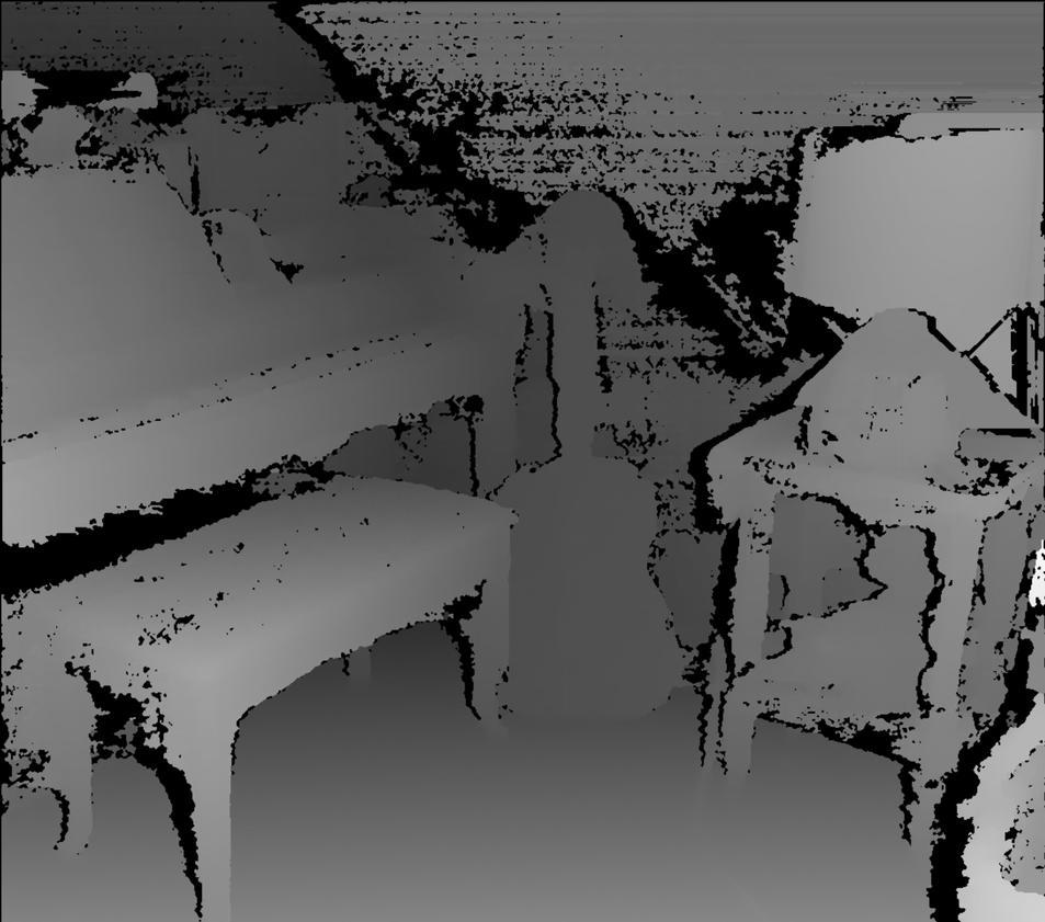
53 5. Results Figure 5.4: The Bad 4.0 result for the aggregation and refinement phase on the dataset shown in Figure 5.1. Figure 5.5: The average Bad 4.0 result for the default algorithm configuration, i.e. the two-pass approximated refinement version, per number of refinement iterations. A direct comparison between the output of StereoSGBM and our algorithm is shown in Figure 5.8. It should be noted that the disparity is calculated at half the input resolution in our tests, while the ground truth is at full resolution (see Section 5.1.1). This makes it a bit harder to visually compare the results, but in general the difference should still be somewhat clear. 43

54 5. Results Figure 5.6: Resulting disparity maps for the Adirondack images for various refinement versions. From left-to-right then top-to-bottom: norefinement, nonapprox, twopassapprox, and twopassapproxidr. The difference in brightness is caused by different normalization and should be ignored. Figure 5.7: Bad 4.0 results from our algorithm compared with the result from OpenCV s StereoSGBM. 44

55 5. Results Figure 5.8: First column is ground truth, middle column is results from the default configuration of our algorithm, last column is results from OpenCV s StereoSGBM. 45

56 5. Results 5.3 Performance This section presents the performance of the algorithm. Various alternatives and optimizations presented in this thesis will be compared against each other. Performance is in this case referring to the running time of the algorithm. Two different metrics are used to measure performance, timemp and timegd. The first of them is simply running time normalized by the number of megapixels in the seconds input images, i.e.. It should be noted that the timemp metric will vary megapixels depending on how big the disparity range is, 100 disparity candidates per pixel will take longer than 10 candidates. For this reason, the latter metric, timegd, is also used. In this metric, the running time is normalized by the number of disparity candidates tested, i.e. seconds. gigapixels disparities Aggregation Phase This section presents the performance results of the aggregation phase. The different aggregation versions for which results were presented in Section are covered here. In addition, the performance of the optimizations covered in Section 4.4 is also included. This includes results for the baseline (twopasssad (Naive)), the simplified support weight expression (twopasssad (Opt SW Expr)), the CUDA SIMD instructions (twopasssad (Opt SIMD)), and the rolling threads optimization (twopasssad (Rolling Threads)). The results are presented in Figure 5.9 and The first figure is the average runtime of the algorithm on a single image pair (in half resolution) from the dataset used (see Figure 5.1). The latter figure presents the results in the timemp and timegd metrics. The non-approximated aggregation version is only included in the figure showing the average running time. Figure 5.9: The average runtime (in milliseconds) for the different aggregation versions. Optimizations are accumulative, i.e. twopasssad (Opt SIMD) also have the optimizations from twopasssad (Opt SW Expr), etc. From Figure 5.9 it is clear that the two-pass approximation is an immense improvement to the performance of the algorithm. As was shown in Section 5.2.1, it is 46

57 5. Results Figure 5.10: Performance results for different aggregation versions. To the left, the timemp metric. To the right, the timegd metric. For the timemp metric 320 disparity candidates were used for each pixel. Optimizations are accumulative, i.e. twopasssad (Opt SIMD) also have the optimizations from twopasssad (Opt SW Expr), etc. also clear that the loss in quality is negligible. However, it should be noted that the non-approximated version has not been as optimized as the two-pass approximation. Most of the optimizations implemented for the two-pass approximation can also be applied to the non-approximated version. By implementing them, the author suspects that it is possible to significantly improve the running time. On the other hand, implementing the census transform might be trickier because shared memory pressure is higher for the non-approximated version. It can be seen that the optimizations presented in Section 4.4 significantly improves the performance. Worth noting is that these optimizations do not affect the quality in any way, they only improve performance. Going from sum of absolute differences to census transform has a non-negligible impact on performance, however reducing the census window size to 7x5 mitigates this Refinement Phase This section presents the performance results of the refinement phase. Specifically, for the refinement versions which results were presented in Section Figure 5.11 shows the average running time for the different versions and a plot showing how the number of refinement iterations affects performance for the default refinement version. Figure 5.12 presents the performance according to the timemp and timegd metrics. 7 iterations of refinement are used for everything. Before these results are studied there are a couple of things to note. Most of the optimizations described in Section 4.4 are applicable for the refinement phase, however they have not been implemented. The author suspects that the performance cost per iteration of refinement can be expected to drop significantly if the optimizations were to be implemented. Another thing to note is that 7 iterations of refinement is used. In practice, this is probably unnecessary. Kowalczuk et al. [4] uses 3 iterations of refinement in their implementation for example. 47

58 5. Results Figure 5.11: In the left figure, the average runtime (in milliseconds) for the different refinement versions (7 iterations of refinement). In the right figure, the average runtime for different number of refinement iterations for the default two-pass approximated refinement version. Figure 5.12: Performance results for different refinement versions. To the left, the timemp metric. To the right, the timegd metric. 7 iterations of refinement. For the timemp metric 320 disparity candidates were used for each pixel. As can be seen in Figure 5.11, there is a linear increase in runtime proportional to the number of refinement iterations. From the numbers presented, it can therefore be calculated that the performance cost for a single pass of two-pass approximated refinement is approximately 21.2 ms Memory Usage This section presents the memory usage and performance tradeoff for different amount of scratch memory. The tradeoff is explained more in depth in Section The sizes of the images in the dataset (see Section 5.1.1) used varies. The average width is 1408 and the average height is 965. This means that one layer in the cost volume approximately uses bytes = 5.18 MiB of memory. The complete cost volume, assuming 320 disparity candidates, then uses a total of 1.66 GiB. During the tests the default configuration is used, with the exception that the refinement phase is disabled. Only a single layer of scratch memory is necessary for the refinement, thus it is not as interesting to look at from this perspective. 48