Color Space Transformations

Transcription

1 Color Space Transformations Philippe Colantoni and Al Introduction This document defines several color concepts and all the mathematic relations used in ColorSpace. The first version of this document has been built 3 years ago using several documents and unfortunately I did not keep all the references. If you find in this document something you write, send me an and I will include your name in the acknowledgment section. 2 Generality 2.1 What is the difference between device dependent and device independent color space? A device dependent color space is a color space where the resultant color depends on the equipment and the set-up used to produce it. For example the color produced using pixel values of rgb = (250,134,67) will be altered as you vary the brightness and contrast on your display. In the same way if you change the red, green and blue phosphors of your monitor will have slightly different characteristics and the color produced will change. Thus RGB is a color space that is dependent on the system being used, it is device dependent. A device independent color space is one where the coordinates used to specify the color will produce the same color wherever they are applied. An example of a device independent color space is the CIE L a b color space (known as CIELAB and based on the human visual system). Another way to define a device dependency is to imagine an RGB cube within a color space representing all possible colors (for example a CIE based color space). We define a color by its values on the three axes, however the exact color will depend on the position of the cube within the perceptual color space, i.e. move the cube (by changing the set-up) and the color will change. Some device dependent color spaces have their position within CIE space defined. They are known as device calibrated color spaces and are a kind of half way house between dependent and independent color spaces. For example, a graphic file that contains colorimetric information, i.e. the white point, transfer functions, 1

2 and phosphor chromaticities, would enable device dependent RGB data to be modified for whatever device was being used - i.e. calibrated to specific devices. 2.2 What is a color gamut? A color gamut is the area enclosed by a color space in three dimensions. It is usual to represent the gamut of a color reproduction system graphically as the range of colors available in some device independent color space. Often the gamut will be represented in only two dimensions. 2.3 What is the CIE System? The CIE has defined a system that classifies color according to the HVS (the human visual system). Using this system we can specify any color in terms of its CIE coordinates. The CIE system works by weighting the spectral power distribution of an object in terms of three color matching functions. These functions are the sensitivities of a standard observer to light at different wavelengths. The weighting is performed over the visual spectrum, from around 360nm to 830nm in set intervals. However, the illuminant, the lighting and the viewing geometry are carefully defined, since these all affect the appearance of a particular color. This process produces three CIE tristimulus values, XYZ, which are the building blocks from which many color measurements are made. 2.4 Gamma and linearity Many image processing operations, and also color space transforms that involve device independent color spaces, like the CIE system based ones, must be performed in a linear luminance domain. By this we really mean that the relationship between pixel values specified in software and the luminance of a specific area on the CRT display must be known. In most cases CRT have a non-linear response. The luminance of a CRT is generally modeled using a power function with an exponent, e.g. gamma, somewhere between 2.2 (NTSC and SMPTE specifications) and 2.8. This relationship is given as follows: luminance voltage γ Where luminance and voltage are normalized. In order to display image information as linear luminance we need to modify the voltages sent to the CRT. This process stems from television systems where the camera and receiver had different transfer functions (which, unless corrected, would cause problems with tone reproduction). The modification applied is known as gamma correction and is given below: NewV oltage = OldV oltage (1/γ) 2

3 (both voltages are normalized and γ is the value of the exponent of the power function that most closely models the luminance-voltage relationship of the display being used.) For a color computer system we can replace the voltages by the pixel values selected, this of course assumes that your graphics card converts digital values to analogue voltages in a linear way. (For precision work you should check this). The color relationships are: R = a.(r ) γ + b G = a.(g ) γ + b B = a.(b ) γ + b where R, G, and B are the normalized input RGB pixel values and R, G, and B are the normalized gamma corrected signals sent to the graphics card. The values of the constants a and b compensate for the overall system gain and system offset respectively (essentially gain is contrast and offset is intensity). For basic applications the value of a, b and γ can be assumed to be consistent between color channels, however for precise applications they must be measured for each channel separately. 3 Tristimulus values 3.1 The concept of the tristimulus values The light that reaches the retina is absorbed by three different pigments that differ in their absorption spectra. Relative absorption spectra of the shortwavelength cone (blue) s(λ), middle-wavelength cone (green) m(λ) and longwavelength cone (red) l(λ) can be see figure 1. Figure 1: Human cones (and rods) absorption spectra If one pigment absorbs a photon which leads to its photoisomeration the information about the wavelength of the photon is lost (principle of univariance). Lights of different wavelengths are able to produce the same degree of isomerations (if their intensities are adjusted properly) and consequently produce equal sensations. The probability of isomeration of one pigment is not correlated with 3

4 the probability of isomeration of another pigment. The probability of isomeration is just determined by the wavelengths of the incident photons. If we do not think about the influences of the spatial and temporal effects that influence perception, the sensation of color is determined by the number of isomerations in the three types of pigments. Therefore colors can be described by just three numbers, the tristimulus values, independent of their spectral compositions that lead to these three numbers. 3.2 The Tristimulus Values The tristimulus values T for a complex light I(λ) (light that is not monochromatic) can be calculated for the specific primaries P with their corresponding color matching functions P i (λ): T 1 = λ P 1 (λ).i(λ).dλ T 2 = 3.3 Consequences λ P 3 (λ).i(λ).dλ T 3 = λ P 2 (λ).i(λ).dλ 1. The amount of excitation of the three pigment types for a complex light stimulus I(λ) can be calculated: S exc = λ s(λ).i(λ).dλ M exc = λ m(λ).i(λ).dλ L exc = λ l(λ).i(λ).dλ 2. The amount of excitation of each pigment type to a stimulus P (λ) can be calculated: S exc = λ s(λ).p (λ).dλ M exc = λ m(λ).p (λ).dλ L exc = λ l(λ).p (λ).dλ Each primary has a defined overlap in the absorption spectra of the three pigments and consequently leads to a defined sensation. An increase in intensity of one primary reduces to the multiplication with a scalar for each pigment. Now, because of the principle of univariance, we can add the influences of the three primaries to the resulting excitations of the three pigment types. 3. Because of 2, there exists a linear transformation between the tristimulus values of a set of primaries and the color space formed by the isomerations of the cone pigments. Tristimulus values describe the whole sensation of a color. There exist a lot of other possibilities to describe the sensation of color. For example it is possible to use something equivalent to cylinder coordinates where a color is expressed by hue, saturation and luminance. If the luminance or the absolute intensity of a color is not of interest then a color can be expressed in chromaticity coordinates. 4

5 3.4 Chromaticity Coordinates In order to calculate the tristimulus values T of a light stimulus due to a set of primaries we need to know the spectral shape of the color matching functions and of the stimulus. The tristimulus values are calculated by the integration of the product of the color matching function and the stimulus over the wavelength. The tristimulus values describe the sensation of the stimulus due to the set of primaries including the absolute intensities of the three primaries needed to match the stimulus. Of course the luminance of that stimulus could be varied without changing the hue and saturation of the stimulus. This is reflected in the chromaticity coordinates c that form a two dimensional space thus luminance is ignored. T 1 T 2 T 3 c 1 = c 2 = c 3 = T 1 + T 2 + T 3 T 1 + T 2 + T 3 T 1 + T 2 + T 3 It is not necessary to mention the third coordinate because: 3.5 Spectrum locus c 1 + c 2 + c 3 = 1 We can read the tristimulus values for the spectral colors as the values of the color matching functions. For complex light stimuli we would have to integrate. After that we can calculate the chromaticity coordinates out of the tristimulus values. In CIE space the tristimulus values are called X, Y and Z, the chromaticity coordinates are called x and y. The curve of the chromaticity coordinates of the spectral colors is called the spectrum locus (fig. 2). The straight line connecting the blue part of the spectrum with the red part of the spectrum does not belong to the spectral colors, but it can be mixed out of the spectral colors just as all colors inside the spectrum locus. 4 Color spaces definitions Color is the perceptual result of light in the visible region of the spectrum, having wavelengths in the region of 380 nm to 780 nm. The human retina has three types of color photoreceptor cells cone, which respond to incident radiation with somewhat different spectral response curves. Because there are exactly three types of color photoreceptor, three numerical components are necessary and theoretically sufficient to describe a color. Because we get color information from image files which contain only RGB values we have only to know for each color space the RGB to the color space transformation formulae. 5

6 Figure 2: CIE 1931 xyy chromaticy diagram 4.1 Computer Graphic Color Spaces Traditionally color spaces used in computer graphics have been designed for specific devices: e.g. RGB for CRT displays and CMY for printers. They are typically device dependent Computer RGB color space This is the color space produced on a CRT display when pixel values are applied to a graphic card or by a CCD sensor (or similar). RGB space may be displayed as a cube based on the three axis corresponding to red, green and blue (see fig. 3(a)) Printer CMY color space The CMY color model stands for Cyan, Magenta and Yellow which are the complements of Red, Green and Blue respectively. This system is used for printing. CMY colors are called subtractive primaries, white is at (0.0, 0.0, 0.0) and black is at (1.0, 1.0, 1.0). If you start with white and subtract no colors, you get white. If you start with white and subtract all colors equally, you get black (see fig. 3(b)). 4.2 CIE XYZ and xyy color spaces The CIE color standard is based on imaginary primary colors XYZ i.e. which don t exist physically. They are purely theoretical and independent of devicedependent color gamut such as RGB or CMY. These virtual primary colors have, however, been selected so that all colors which can be perceived by the 6

7 (a) RGB color space (b) CMY color space Figure 3: Visualization of RGB and CMY color spaces human eye lie within this color space. The XYZ system is based on the response curves of the three color receptors of the eye s. Since these differ slightly from one person to another person, CIE has defined a standard observer whose spectral response corresponds more or less to the average response of the population. This objectifies the colorimetric determination of colors. XYZ (fig. 4(a)) is a 3D linear color space, and it is quite awkward to work in it directly. It is common to project this space to the X + Y + Z = 1 plane. The result is a 2D space known as the CIE chromaticity diagram (see fig. 2). The coordinates in this space are usually called x and y and they are derived from XYZ using the following equations: x = X X + Y + Z y = Y X + Y + Z z = Z X + Y + Z As the z component bears no additional information, it is often omitted. Note that since xy space is just a projection of the 3D XYZ space, each point in xy corresponds to many points in the original space. The missing information is luminance Y. Color is usually described by xyy coordinates, where x and y determine the chromaticity and Y the lightness component of color (fig. 4(b)) RGB to CIE XYZ Conversion There are different mathematical models to transform RGB device dependent color to XYZ tristimulus values. Conversion from RGB to XYZ can take the form of a simple matrix transformation (equ. 2) or a more complex transformation depending of the hardware used (e.g. to acquire or to display color information). (1) 7

8 In this section we will define how to compute a linear transformation model. This model may by a correct approximation for CCD sensor (RGB to XYZ transform) and CRT display (XYZ to RGB transform). But do not forget, this is only an approximate model. R G B = A. X Y Z We can use for example this transformation: R G B = and the inverse transform simply uses the inverse matrix. X Y Z = (2). 1 X Y Z This is all very useful, but the interesting question is Where do these numbers come from?. Figuring out the numbers to put in the matrix is the hard part. The numbers depend on the color system of the output device we are using. The important parts of a color system are the x and y chromaticity coordinates and the luminance component of the primaries (xyy ). However, if we don t know the Y values, which is often the case, then we have a problem. However, we can solve this problem if we know the chromaticity coordinates of the white point. In the previous example we have used a the color system which has the following specifications:. Coordinate x Red y Red x Green y Green x Blue y Blue Value R G B Coordinate x W hite y W hite Y W hite Value These terms will be abbreviated to x r, y r, x g, y g, x b, y b, x w, y w and Y w. We know already that the relation 1 links the tristimulus values to the chromaticity coordinates. We can transform these relations: X = x y Y Z = z y Y The first step is to use these relationships to determine the luminance Y values. So we can calculate the tristimulus values as follows 8

9 X r = Y r y r x r X g = Y g y g x g X b = Y b y b x b Y r = Y r Y g = Y g Y b = Y b Z r = Yr y r z r Z g = Y g y g z g For the tristimulus values of the white point: Z b = Y b y b z b X w = x w yw Y w = Y w Z w = z w yw We now make the assumption that the sum of full intensity values of red green and blue will be white. Using this assumption we can write this relationship: X w = X r + X g + X b Y w = Y r + Y g + Y b Z w = Z r + Z g + Z b We can then substitute the previous equations to the current one and then rewrite this latter as a matrix relationship: x w x yw Y w r x g x b y r y g y b Y w = Y r Y g z w y w Y w Y b z r y r z g y g This matrix can be re-written as follows: Y x r x g x b r y r y g y b Y g = Y b z r y r z g y g z b y b z b y b 1. x w yw Y w Y w z w y w Y w We now have the luminance values Y r, Y g, Y b and we can substitute these values into the previous equations to find X r, X g, X b, Z r, Z g, and Z b. The final step is to define the relationship between tristimulus values and RGB values as follows. The RGB matrix R should be the result of a multiplication of the conversion matrix C by the tristimulus matrix T : =????????? X w X r X g X b Y w Y r Y g Y b Z w Z r Z g Z b Then the conversion matrix can be calculated as follows C = R T T (T T T ) 1 If we follow this procedure using the values given in the previous example then we arrive at the following solution: C =

10 (a) XYZ color space (b) xyy color space Figure 4: Visualization of XYZ and xyy color spaces Chromaticity coordinates of phosphors Name x r y r x g y g x b y b White point Short-Persistence N/A Long-Persistence N/A NTSC Illuminant C EBU Illuminant D65 Dell K SMPTE Illuminant D65 HB LEDs x w =.31 y w = Standard white points Name x w y w Illuminant A Illuminant B Illuminant C Illuminant D Direct Sunlight Light from overcast sky Illuminant E 1/3 1/3 4.3 A better model for RGB to CIE XYZ conversion ColorSpace enables user to apply a more accurate model for RGB to CIE XYZ conversion. This model (equ. 3) includes an offset suitable to calibrate CCD or CMOS sensors. 10

11 X Y Z = A. R G B + X offset Y offset Z offset (3) 4.4 CIE L a b and CIE L u v color spaces There are based directly on CIE XYZ (1931) and are another attempt to linearize the perceptibility of unit vector color differences. there are non-linear, and the conversions are still reversible. Coloring information is referred to the color of the white point of the system. The non-linear relationships for CIE L a b (see equ. 4 and fig. 5(a)) are not the same as for CIE L u v (see equ. 7 and fig. 5(b)), both are intended to mimic the logarithmic response of the eye. L = 116 ( Y ) 1 3 Y 0 L = ( ) Y [ Y 0 ] a = 500 f( X X 0 ) f( Y Y 0 ) [ ] b = 200 f( Y Y 0 ) f( Z Z 0 ) 16 if Y Y 0 > if Y Y (4) with { f(u) = U 1 3 if U > f(u) = 7.787U + 16/116 if U and U(X, Y, Z) = 4X X + 15Y + 3Z et V (X, Y, Z) = 9Y X + 15Y + 3Z (5) (6) L = 116 ( Y ) 1 3 Y 0 ( ) Y Y 0 16 if Y Y 0 > L = ] u = 13L [U(X, Y, Z) U(X 0, Y 0, Z 0 ) [ ] v = 13L V (X, Y, Z) V (X 0, Y 0, Z 0 if Y Y (7) 4.5 Color spaces used in video standards Y UV and Y IQ are standard color spaces used for analogue television transmission. Y UV is used in European TVs (see fig. 6(a)) and Y IQ in North American TVs (NTSC) (see fig. 6(b)). Y is linked to the component of luminance, and U, V and I, Q are linked to the components of chrominance. Y comes from the standard CIE XYZ. 11

12 (a) L a b color space (b) L u v color space Figure 5: Visualization of L a b and L u v color spaces (a) Y UV color space (b) Y IQ color space Figure 6: Visualization of Y UV and Y IQ color spaces 12

13 RGB to Y U V transformation Y = R G B U = R G B V = R G B RGB to Y IQ transformation Y = R G B I = R G B Q = R G B With these formulae the Y range is [0; 1], but U, V, I, and Q can be as well negative as positive. Y CbCr (see fig. 4.5) is a color space similar to Y UV and Y IQ. The transformation formulae for this color space depend on the recommendation used. We use the recommendation Rec which gives the value for red, the value for green and the value for blue. Figure 7: Y CbCr color space RGB to Y CbCr transformation Y = R G B Cb = R G B Cr = R G B 4.6 Linear transformations of RGB I 1 I 2 I 3 color space Ohta [3] introduced, after a colorimetric analysis of 8 images, this color space. This color space is a linear tranformation of RGB (see fig ). 13

14 Figure 8: I 1 I 2 I 3 color space RGB to I 1 I 2 I 3 transformation I 1 = 1 3 (R + G + B) I 2 = 1 2 (R B) I 3 = 1 4 (2G R B) LSLM color space This color space is a linear transformation of RGB based on the opponent signals of the cones: black white, red green, and yellow blue (see fig ). RGB to LSLM transformation L = 0.209(R 0.5) (G 0.5) (B 0.5) S = 0.209(R 0.5) (G 0.5) 0.924(B 0.5) LM = 3.148(R 0.5) 2.799(G 0.5) 0.349(B 0.5) 4.7 HSV and HSI color spaces The representation of the colors in the RGB and CMY color spaces are designed for specific devices. But for a human observer, they have not accurate definitions. For user interfaces a more intuitive color space is preferred. Such color spaces can be: HSI ; Hue, Saturation and Intensity, which can be thought of as a RGB cube tipped up onto one corner (see fig. 10(b) and equ. 8). 14

15 Figure 9: LSLM color space (a) HSV color space (b) HSI color space Figure 10: Visualization of HSV and HSI 15

16 RGB to HSI transformation H = arctan( β α ) S = α 2 + β 2 I = (R + G + B)/3 (8) with { α = R 1 2 (G + B) β = 3 2 (G B) There is different way to compute the HSV (Hue, Saturation and Value) color space [4]. We use the following algorithm 4.7. RGB to HSV transformation 1 if (R > G) then Max = R; Min = G; position = 0; 2 else Max = G; Min = R; position = 1; 3 fi 4 if (Max < B) then Max = B; position = 2 fi 5 if (Min > B) then Min = B; fi 6 V = Max; 7 if (Max 0) then S = Max Min Max ; 8 else S = 0; 9 fi 10 if (S 0) then 11 if (position = 0) 12 then H = 1 + G B Max Min ; 13 else if (position = 1); 14 then H = 3 + B R Max Min ; 15 else H = 5 + R G Max Min ; 16 fi 17 fi The polar representation of HSV (see fig. 11(a)) and HSI (see fig. 11(b)) color spaces leads a new visualization model of these color spaces (suitable for color selection). 4.8 LHC and LHS color spaces The L a b (and L u v ) has the same problem as RGB, they are not very interesting for user interface. That s why you will prefer the LHC equa. 9 (and LHS equa. 10), a color space based on L a b (and LHS). LHC stand for Luminosity, Chroma and Hue. 16

17 (a) HSV color space (polar representation) (b) HSI color space (polar representation) Figure 11: Visualization of HSV and HSI color spaces (polar representation) L a b to LHC transformation L = L C = a 2 + b 2 H = 0 whether a = 0 H = (arctan(b /a ) + k.π/2)/(2π) whether a 0 (add π/2 to H if H < 0) and k = 0 if a >= 0 and b >= 0 or k = 1 if a > 0 and b < 0 or k = 2 if a < 0 and b < 0 or k = 3 if a < 0 and b > 0 L u v to LHS transformation L = L S = 13 (u u w) 2 + (u u w) 2 H = 0 whether u = 0 H = (arctan(v /u ) + k.π/2)/(2π) whether u 0 (add π/2 to H if H < 0) and k = 0 if u >= 0 and v >= 0 or k = 1 if u > 0 and v < 0 or k = 2 if u < 0 and v < 0 or k = 3 if u < 0 and v > 0 (9) (10) In order to have a correct visualization (with a good dynamic) of LHS and LHC color spaces we used the following color transformations: 17

18 L a b to LHC transformation used in ColorSpace L = L C = a 2 + b 2 H = 0 whether a = 0 H = 180 π (π + arctan( b a ) L u v to LHS transformation used in ColorSpace L = L S = 1.3 (u u w) 2 + (v vw) 2 H = 0 whether u = 0 H = 180 π (π + arctan( v u ) (11) (12) (a) LHC color space (b) LHS color space Figure 12: Visualization of LHC and LHS color spaces 4.9 Spectral (λsy ) color space λsy is a color space representation based on brightness, dominant wavelength and saturation attributes. λsy color coordinates are defined from xyy color coordinates. Let us consider the xy chromaticy diagram given by Figure 13(b). Then, any real color X that lies within the region enclosed by the spectrum locus line and upper the lines BW and W R can be considered to be a mixture of illuminant W and spectrum light of its dominant wavelength λ d which is determined by extending the line W X until it intersects the spectrum locus [9]. Any color Y that lies on the opposite side of the illuminant point and below the lines BW and W R can be described both by a dominant wavelength λ d and 18

19 λd Green λ d Green x x smax Spectrum locus x c Spectrum locus x λa d White White Blue Red Blue y y s max Red (a) (b) (c) (d) Figure 13: λsy color space transformation. 19

20 by its complementary wavelength λ c d which is determined by extending the line Y W until it intersects the line BR (i.e. the purple line). The saturation S is determined in the xy chromaticity diagram, either by the relative distance of the sample point and the corresponding spectrum point from the illuminant point, either by the relative distance of the sample point and the corresponding purple point from the illuminant point. 5 Decorrelated hybrid color spaces The basic idea of hybrid color spaces is to combine either adaptively, either interactively, different color components from different color spaces to: (a) increase the effectiveness of color components to discriminate color data, and (b) reduce rate of correlation between color components [2]. It is established that we can all the more reduce, from K to 3, the number of color dimensions that: (a) most of color spaces are linked the ones to the others, either by linear transformations or by non-linear transformations, and (b) all color spaces are defined by a 3 dimensional system. (a) (b) (c) (d) (e) (f) (g) (h) (i) (j) Figure 14: (a) RGB Color image, made of 6 regions (Brown, Orange, Yellow, Pink, Green and Dark Green), projected on different color components. (b), (c), (d) R, G, B projections. Among the three R, G, B color components, at most 3 regions can be identified with the component G. (e), (f), (g) Y, C b, C r projections. Among the three Y, C b, C r color components, at most 3 regions can be identified with the component Y. (h), (i), (j) H, S, V projections. Among the three H, S, V color components, at most 3 regions can be identified with the component H. In combining G, Y, H color components, all regions can be identified. Considering that there is a high redundancy between colors components it is, in a general way, quite difficult to define criteria of analysis to compute au- 20

21 tomatically the most relevant color components corresponding to a selected set of color components. That is the reason why, in order to build a hybrid color space, based on K color components, from K selected color components, such as K << K (see Figure 14), we propose the following method: (1) select K color components, by using a specific interface which enables the user to weight each selected color components, and build the corresponding image of dimension K, (2) compute the covariance matrix (of size K K) of K color components selected, (3) compute the eigenvectors and the eigen values of this matrix, (4) reduce to K the number of color components in computing the K most significant eigen values of the covariance matrix from a principal component analysis (PCA). Next, the three first principal components computed (i.e. the decorrelated hybrid colors components) are used to compute the 3D representation which best characterizes the image studied (see Figure 15). (a) Original Image (b) 3D representation of the hybrid colors Figure 15: Decorrelated hybrid color space visualization Figures 16 shows some 3D visualization of decorrelated hybrid color spaces in different configurations in 16(b) 1, 16(c) 1 and 16(d) 2 1 Using Components R,G and B of RGB, X and Y of XYZ, L, M and S of LMS, cos of λsy P olar, without weight 1 Using Components L and a of L a b, H and C of LHC, H and S of HSI, without weight 2 Using Components Y of xyy, L of L a b,l of LHC, I of HSI, without weight 21

22 (a) Parrot image (b) (c) (d) Figure 16: Decorrelated hybrid color spaces examples on parrot image 22

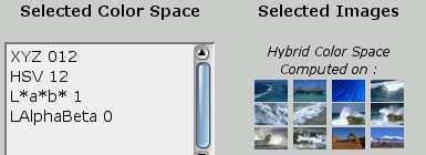
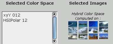
23 6 Decorrelated hybrid color spaces applied to image database 6.1 Decorrelated hybrid color spaces: an extension We have introduced the hybrid construction scheme in the precedent paragraph, based on one initial image. This strategy can be easily applied to a list of images, considering the set of images as one unique image. We will use the following notations, and we will suppose (for simplicity of formulæ only) all color spaces are normalized. S the set of n images and S l the l-th image. K the set of selected color spaces components and K i the i-th component. K l i (x, y) the corresponding value of pixel (x, y) of component K i of image S l. Size (S l ) the size in pixel of the image S l. Let introduce the Sum and Cross matrix, defined by: Sum l i = xy S l K l i(x, y) Cross l ij = xy S l K l i(x, y) K l j(x, y) We note, that for one image S l, the covariance is then defined by: Cov l ij = Crossl ij Size (S l ) Suml i Size (S l ) Then, to expand the formula to n images: 1 l n Cov ij = Crossl ij 1 l n Size (S l) 1 l n Suml i 1 l n Size (S l) Suml j Size (S l ) 1 l n Suml j 1 l n Size (S l) At this point, the computation of the hybrid color space follows the previously cited steps: 4. principal component analysis; 5. selection of the 3 most significant axis. We have developed via ICobra and ColorSpace applications a web interface system 3 [14] to manage these hybrid color spaces. The process is divided in two steps: 3 Available at: 23

24 Off-line computation. This part intends to compute the main portion of calculus required by the hybrid color space computation. Online interface. This part intends, via the interface, to select color spaces components and images, to complete the calculus, and, then, to show the selected image in the computed hybrid space. Before describes rapidly these two parts, we can note: all color spaces are normalized during the computation (there is a scale rapport from 1 to 200 between some spaces); the transfer values (primaries and white settings) used are, at this moment, still approximation. 6.2 Off-line computation Figure 17: Off-line scheme The figure 17 illustrates the off-line computation. For each image, we will compute and store: for each couple of color spaces components, the Cross value corresponding. It results a m m matrix, where t is the number of possible color spaces components, presently 72 (3 24) components. for each color spaces components, the Sum value corresponding. It results a vector of size m. the size of image. 6.3 Online interface As shown in 17 the application may be split into several sections: World Wide Web Interface, as figure 19 illustrates. It permits: to browse the different image databases; to select by clicks a list of images. An empty list means that the decorrelated hybrid color space is computed on self-image, as usual; 24

25 Figure 18: Overall online scheme Figure 19: WWW interface 25

26 to select a list of color spaces components; to choose the mode of visualization: 2D image, 3D, or 3D histogram; to launch ColorSpace with the selected parameters; A computational part: the final covariance matrix is computed, using pre-calculated data; A CSI file generation: a csi file (Color Space Interface) is generated, including all settings and information in order to compute the PCA and displaying the selected visualization; ColorSpace launching: ColorSpace is launched by the browser (application/csi mime-type bind) with the csi file as parameter. The software computes the PCA, and renders the selected visualization. Figure 20 illustrates this tool within some screenshots using different images and color spaces components. 7 References and lectures [1] P. Colantoni and A. Trémeau, 3d visualization of color data to analyze color images, in The PICS Conference, (Rochester, USA), May [2] N. Vandenbrouke, L. Macaire, and J. G. Postaire, Color pixels classification in a hybrid color space, in Proceedings of IEEE, pp , [3] Y. I. Ohta, T. Kanade, and T. Sakai, Color information for region segmentation, Computer Graphics and Image Processing, vol. 13, pp , [4] D. F. Rogers, Procedural Elements for Computer Graphics. Mc Graw Hill, [5] G. A. Agoston, Color Theory and its Application in Art and Design. Optical Sciences, Springer-Verlag, [6] CIE, Parametric effects in colour-difference evaluation, Tech. Rep. 101, Bureau Central de la CIE, [7] CIE, Technical collection 1993, tech. rep., Bureau Central de la CIE, [8] CIE, Industrial colour-difference evaluation, Tech. Rep. 116, Bureau Central de la CIE, [9] D. L. MacAdam, Color Measurement, theme and variation. Optical Sciences, Springer-Verlag, second revised ed., [10] G. Wyszecki and W. S. Stiles, Color Science: Concepts and Methods, Quantitative Data and Formulae. John Wiley & sons, second ed.,

27 (a) Original image (b) Selected components (c) Decorrelated hybrid color and images space representation list (d) (e) (f) (g) (h) (i) Figure 20: Decorrelated hybrid color spaces: some examples 27

28 [11] H. R. Kang, Color Technology for Electronic Imaging Devices. SPIE Optical Engineering Press, [12] K. N. Plataniotis and A. N. Venetsanopoulos, Color Image Processing and Application. Springer, [13] R. Hall, Illumination and Color in Computer Generated Imagery. Springer-Verlag, [14] J. D. Rugna, P. Colantoni, and N. Boukala, Hybrid color spaces applied to image database, vol. 5304, pp , Electronic Imaging, SPIE,