MIGRATION-VELOCITY ANALYSIS USING IMAGE-SPACE GENERALIZED WAVEFIELDS

Transcription

1 MIGRATION-VELOCITY ANALYSIS USING IMAGE-SPACE GENERALIZED WAVEFIELDS A DISSERTATION SUBMITTED TO THE DEPARTMENT OF GEOPHYSICS AND THE COMMITTEE ON GRADUATE STUDIES OF STANFORD UNIVERSITY IN PARTIAL FULFILLMENT OF THE REQUIREMENTS FOR THE DEGREE OF DOCTOR OF PHILOSOPHY Claudio Guerra July 2010

2 Copyright by Claudio Guerra 2010 All Rights Reserved ii

3 I certify that I have read this dissertation and that, in my opinion, it is fully adequate in scope and quality as a dissertation for the degree of Doctor of Philosophy. (Biondo Biondi) Principal Adviser I certify that I have read this dissertation and that, in my opinion, it is fully adequate in scope and quality as a dissertation for the degree of Doctor of Philosophy. (Jon F. Claerbout) I certify that I have read this dissertation and that, in my opinion, it is fully adequate in scope and quality as a dissertation for the degree of Doctor of Philosophy. (Jerry Harris) Approved for the University Committee on Graduate Studies. iii

4 iv

5 Abstract An accurate depth-velocity model is the key for obtaining good quality and reliable depth images in areas of complex geology. In such areas, velocity-model definition should use methods that describe the complexity of wavefield propagation, such as focusing and defocusing, multiple arrivals, and frequency-dependent velocity sensitivity. Wave-equation tomography in the image space has the ability to handle these issues because it uses wavefields as carriers of information. However, its high cost and low flexibility for parametrizing the model space has prevented its routine industrial use. This thesis aims at overcoming those limitations by using new wavefields as carriers of information: the image-space generalized wavefields. These wavefields are synthesized by using a pre-stack generalization of the exploding-reflector model. Cost of wave-equation tomography in the image space is decreased because only a small number of image-space generalized wavefields are necessary to accurately describe the kinematics of velocity errors and because these wavefields can be easily used in a target-oriented way. Flexibility is naturally incorporated into wave-equation tomography in the image space by using these wavefields because their modeling have as the initial conditions some key selected reflectors, allowing a layer-based parametrization of the model space. To use the image-space generalized wavefields in wave-equation tomography in the image space, the method is extended from the shot-profile domain to the image-space generalized-sources domain. In this new domain, the velocity updates are very fast. Migration with the optimized velocity model provides good quality and reliable depth v

6 images, as can be seen in a 3D-field data example. vi

7 Preface The electronic version of this report 1 makes the included programs and applications available to the reader. The markings ER, CR, and NR are promises by the author about the reproducibility of each figure result. Reproducibility is a way of organizing computational research that allows both the author and the reader of a publication to verify the reported results. Reproducibility facilitates the transfer of knowledge within SEP and between SEP and its sponsors. ER denotes Easily Reproducible and are the results of processing described in the paper. The author claims that you can reproduce such a figure from the programs, parameters, and makefiles included in the electronic document. The data must either be included in the electronic distribution, be easily available to all researchers (e.g., SEG-EAGE data sets), or be available in the SEP data library 2. We assume you have a UNIX workstation with Fortran, Fortran90, C, X-Windows system and the software downloadable from our website (SEP makerules, SEPScons, SEPlib, and the SEP latex package), or other free software such as SU. Before the publication of the electronic document, someone other than the author tests the author s claim by destroying and rebuilding all ER figures. Some ER figures may not be reproducible by outsiders because they depend on data sets that are too large to distribute, or data that we do not have permission to redistribute but are in the SEP data library, or that the rules depend on commercial packages such as Matlab or Mathematica html vii

8 CR denotes Conditional Reproducibility. The author certifies that the commands are in place to reproduce the figure if certain resources are available. The primary reasons for the CR designation is that the processing requires 20 minutes or more. NR denotes Non-Reproducible figures. SEP discourages authors from flagging their figures as NR except for figures that are used solely for motivation, comparison, or illustration of the theory, such as: artist drawings, scannings, or figures taken from SEP reports not by the authors or from non-sep publications. Some 3D synthetic data examples associated with this report are classified as NR because they were generated externally to SEP and only the results were released by agreement. Our testing is currently limited to LINUX 2.6 (using the Intel Fortran90 compiler) and the SEPlib distribution, but the code should be portable to other architectures. Reader s suggestions are welcome. For more information on reproducing SEP s electronic documents, please visit viii

9 Acknowledgments ix

10 Contents Abstract v Preface vii Acknowledgments ix 1 Introduction 1 2 Pre-Stack Exploding-Reflector Model 10 3 Image-space phase-encoded wavefields 53 4 MVA using image-space generalized sources D field-data example Conclusions 145 x

11 List of Tables xi

12 List of Figures 1.1 Migration of the original 375 shot-profiles Horizontal plane-wave synthesis. a) generalized source function, b) generalized receiver gather, and c) areal-shot migration Horizontal plane-wave at depth 2300 m by the controlled illumination method. a) generalized source function, b) generalized receiver gather, and c) areal-shot migration Random-phase encoding combining every 20 shots. a) generalized source function, b) generalized receiver gather, and c) areal-shot migration Shot-profile migrated images of Marmousi obtained with: a) An initial velocity model, which is inaccurate below the top of the anticline at depth 1700 m, b) a velocity model optimized with ISWET, using 11 pairs of image-space generalized sources synthesized from 12 selected reflectors and collected at depth 1500 m a) Shot-profile migration of 380 off-end shots 24 m apart. b) Shotprofile migration of 23 off-end shots 384 m apart. Both images were computed with the correct velocity model. Notice slanted lines present in Figure 2.1b xii

13 2.2 a) Shot-profile migration of 95 areal shots resulting from the combination of 4 shot profiles 2256 m apart. b) Shot-profile migration of 23 areal shots resulting from the combination of 16 shot profiles 564 m apart. Both images were computed with the correct velocity model. Notice crosstalk occurring periodically in the SODCIG of Figure 2.2b Angle-domain common-image gathers (top) and residual moveout panels (bottom). Left: full migration. Middle: migration of 23 sampled shots. Right: migration of the combined shots. Crosstalk resulting from the combination of many shots destroys the velocity information Shot-profile migration of 401 split-spread shots 10 m apart with a 10% slower velocity. The model consists of a horizontal reflector embedded in constant velocity of 1000 m/s Data synthesized by PERM having as the initial condition the SODCIG at x m = 0 m. a) The receiver wavefield. b) The source wavefield Areal-shot migration of PERM data shown in Figure 2.5 with a 10% slower velocity. By comparing with Figure 2.4 we see that far subsurfaceoffsets are not properly imaged Areal-shot migration of PERM data having a set of isolated SODCIGs around x m = 0 m as the initial condition with a 10% slower velocity. By comparing with Figure 2.4 we see that the kinematics of far subsurfaceoffsets is properly recovered ADCIGs selected at x m = 0 m. a) Computed from the shot-profile migration; b) computed from the areal-shot migration of one pair of PERM data modeled from the SODCIG at x m = 0 m; and c) computed from the areal-shot migration of pairs of PERM data modeled from a set of SODCIGs around x m = 0 m. Notice that although the kinematics are similar, the amplitudes in c) better match those of a). 27 xiii

14 2.9 Areal-shot migration of PERM data having a set of isolated SODCIGs around x m = 0 m as the initial condition with the correct velocity. Energy nicely focuses at zero-subsurface offset Geometry for the computation of SODCIGs. Source, receiver and image points are labeled with S, R and I, respectively. The subscript hx corresponds to subsurface offsets computed with horizontal shift. The subscript hg corresponds to subsurface offsets computed by shifting along the apparent geological dip α. a) Underestimated velocity, and b) overestimated velocity. Modified from Biondi and Symes (2004) Shot-profile migration of 801 split-spread shots 10 m apart with velocity 10% slower than the true velocity. The model is represented by a 20 dipping reflector and a horizontal reflector at a depth of 2500 m embedded in a medium with a constant velocity of 1000 m/s Data synthesized by PERM having as the initial condition the dipping reflector in the SODCIG at x m = 0 m. a) The receiver wavefield. b) The source wavefield Areal-shot migration of PERM data shown in Figure 2.12 using the correct velocity. The horizontal reflector is focused at zero-subsurface offset, but the dipping reflector shows residual curvature Areal-shot migration with correct velocity of PERM data having a set of isolated SODCIGs around x m = 0 m as the initial conditions. As in Figure 2.13, the horizontal reflector is focused at zero-subsurface offset, but the dipping reflector shows residual curvature Initial conditions for modeling a) source and b) receiver wavefields. The dipping reflector is oriented in opposite directions in the SODCIG. Rotation affects neither the horizontal reflector nor the-zero subsurface offset, as can be seen in the right panels xiv

15 2.16 Dip-independent PERM data for the dipping reflector from the rotated SODCIG at x m = 0 m. a) The receiver wavefield. b) The source wavefield Areal-shot migration with the correct velocity of dip-independent PERM data having the rotated the SODCIGs at x m = 0 m as the initial condition. The SODCIG on the left is selected at the horizontal position where the dipping reflector was laterally shifted to. Compare with Figure The dipping reflector is now focused in contrast to the image in Figure 2.13, where it shows residual curvature Areal-shot migration with correct velocity of dip-independent PERM data having a set of rotated SODCIGs around x m = 0 m as the initial conditions. Compare with Figure The focusing of the dipping reflector is greatly improved when using the rotated initial conditions ADCIGs of images computed with the correct migration velocity using PERM data having: a) non-rotated initial conditions, and b) rotated initial conditions. Note the residual move-out in a) and the flatter response in b) Areal-shot migration of PERM data synthesized from sets of SOD- CIGs selected with sampling period of 163 SODCIGs. Notice that no crosstalk is generated when the sampling period is larger than twice the subsurface-offset range The initial conditions for synthesizing PERM data from CAM images can be specified as in b) because no pre-stack information exists in the cross-line direction, in contrast with the full azimuth situation in a).. 47 xv

16 2.22 Common-azimuth migration of 3D-Born data modeled from a 30 dipping reflector with 45 azimuth with respect to the acquisition direction. The panel in the middle is the in-line at the zero-subsurface offset, and y = 600 m (Figure 2.22a) and y = 1000 m (Figure 2.22b). The panel on the right is the cross-line at the zero-subsurface offset, and x = 750 m D-PERM receiver wavefield. The left panel is the in-line at y = 1200 m, the right panel is the cross-line at x = 1400 m, and the top panel is the time-slice at t = 0.5 s D-areal-shot migration of PERM data from non stretched subsurface offset SODCIGs. The panel in the middle is the in-line at the zerosubsurface offset, and y = 600 m (Figure 2.22a) and y = 1000 m (Figure 2.22b). The panel on the right is the cross-line at the zerosubsurface offset, and x = 750 m. Compare with Figure 2.22 and D-areal-shot migration of PERM data from stretched subsurface offset SODCIGs. The panel in the middle is the in-line at the zero-subsurface offset, and y = 600 m (Figure 2.22a) and y = 1000 m (Figure 2.22b). The panel on the right is the cross-line at the zero-subsurface offset, and x = 750 m. Compare with Figure 2.22 and Areal-shot migration of PERM data synthesized from a set of SOD- CIGs selected with sampling period of 163. The two reflectors are simultaneously injected to the model. Notice the reflector crosstalk, labeled with C, resulting from the cross-correlation of the wavefields from the horizontal reflector with that from the dipping reflector xvi

17 3.2 Snapshots of propagation of wavefields used to compute the image of Figure 3.1. Wavefields are labeled D (Downgoing) for the source wavefield and U (Upgoing) for the receiver wavefield. The panels on the left are selected at horizontal positions where the crosstalk occurs in Figure 3.1. The panels on the right are taken at the propagation time when the wavefields cross on the left panel Areal-shot migration of PERM data synthesized from sets of SODCIGs selected with sampling period of: a) 41 and, b) ADCIGs (top) and ρ-panels (bottom) corresponding to images computed by wavefields modeled with sampling period of: a) 41, b) 81, and c) 163. Velocity information has been destroyed by the crosstalk in a) and b) Areal-shot migration using the time-windowed imaging condition (equation 3.2). The reflector crosstalk is completely eliminated Velocity models for the Marmousi example: a) Smooth velocity model used to model the Born data. b) Background velocity model used to migrate the Born data, and to model and migrate PERM data a) Pre-stack image computed with the background velocity model. b) Selected reflectors from the background image to perform modeling of wavefields Rotated initial conditions for modeling: a) source wavefields, and b) receiver wavefields PERM wavefields for the Marmousi example: a) Receiver wavefield. b) Source wavefield xvii

18 3.10 Pre-stack image computed with PERM wavefields and background velocity model using: a) the conventional imaging condition (equation 2.12), and b) the time-windowed imaging condition (equation 3.2). Reflector crosstalk is avoided when reflectors are sufficiently separated. However, some residual crosstalk is still present (RC). Notice the phase difference of the PERM image due to the squaring of the wavelet when compared to the windowed reflectors of Figure 3.7b ISPEW from different random realizations initiated at the same SOD- CIGs for the Marmousi example: a,c) Receiver wavefields. b,d) Source wavefields Pre-stack images computed with: a) Four random realizations of IS- PEW, and b) a single random realization ADCIGs (top) and ρ-panels (bottom) corresponding to images computed by: a) Shot-profile migration of 360 shot gathers, b) areal-shot migration of 35 PERM wavefields using the time-windowed imaging condition, c) areal-shot migration of 44 ISPEW corresponding to four random realizations, and d) areal-shot migration of 11 ISPEW corresponding to a single random realization. The moveout information is basically the same Marmousi velocity models: a) True velocity model. b) Backgroundvelocity model computed by smoothing and scaling down the true model below the horizon indicated by the black line Snapshots of background: a) source, and b) receiver wavefields Background image and SODCIGs computed with the background wavefields of Figure Perturbed image computed with equation Snapshots of perturbed: a) source, and b) receiver wavefields xviii

19 4.6 Slowness perturbation from back-projected image perturbations Selected reflectors used to model the image-space generalized source and receiver gathers Snapshots of image-space generalized background wavefields: a) source, and b) receiver wavefields Background image computed with the image-space generalized background wavefields of Figure Perturbed image computed with equation Snapshots of image-space generalized perturbed wavefields: a) source, and b) receiver Slowness perturbation from back-projected image perturbations computed with 35 ISPEW a) Initial and b) final background image for the optimization with 11 ISPEW a) Initial and b) final background image for the optimization with 35 ISPEW Evolution of the objective function for the 11-ISPEW case (blue diamonds) and 35-ISPEW case (red squares) Optimized velocity models for: a) the 11-ISPEW case, and b) 35- ISPEW case a) Smoothed version of the true velocity model, b) histogram of the velocity ratio between the smoothed true velocity model and the initial velocity model, c) histogram of the velocity ratio between the smoothed true velocity model and the 11-ISPEW optimized velocity model, and d) histogram of the velocity ratio between the smoothed true velocity model and the 35-ISPEW optimized velocity model xix

20 4.18 Images computed with shot-profile migration using the optimized velocity models of Figure 4.16: a) the 11-ISPEW case, and b) 35-ISPEW case Image computed with shot-profile migration using the true velocity model a) Offset azimuth cross-plot, b) azimuth histogram, c) in-line offset histogram, and d) cross-line offset histogram Fold of coverage plots: a) full offset, b) m offset, c) m offset, and d) m offset Time slices through the trace envelope for different offset cubes from the regularized data: a) offset 200m, b) offset 1200 m, c) offset 2400 m, and d) offset 3000 m Slices through the IFP velocity model Slices through the initial velocity model used in 3D-ISWET Slices through an initial velocity model generated with the same procedures as that for Figure 5.5, except for the velocity above the chalk, which is the original velocity Image computed with the velocity model of Figure 5.6. The top panel is the zero-subsurface offset section and the panel at the bottom are the SODCIGs Image computed with the velocity model of Figure 5.5. The top panel is the zero-subsurface offset section and the panel at the bottom are the SODCIGs. Compare with Figure Slices through the CAM image with the initial velocity model of Figure 5.5. Notice poorly collapsed diffractions close to the salt flank (A and D), and poorly imaged faults (B and C) caused by migrating with an inaccurate velocity xx

21 5.10 In-line 3180 of the CAM image with the initial velocity model of Figure 5.5. On the top is the zero-subsurface offset section, and at the bottom ADCIGs. Notice the strong residual moveout on the ADCIGs. The continuous blue line is the top of chalk, and the dashed blue line it the base of chalk Slices through the mask operator to select the base of chalk: a) for the zero subsurface offset, and b) for the in-line A pair of 3D source (a) and receiver (b) ISPEW computed for the base of chalk DSO slowness perturbation without smoothing and without extracting the signaled square root from the initial conditions for the modeling of 30 pairs of ISPEW DSO slowness perturbation without smoothing and extracting the signaled fourth root of the gradient DSO slowness perturbation after B-spline smoothing the DSO slowness perturbation of Figure Evolution of the DSO objective function for the first run of ISWET for the base of chalk In-line 3520 of the initial background image of the first run of ISWET for the base of chalk In-line 3520 of the background image computed with the optimized velocity model of the first run of ISWET for the base of chalk Slices through the optimized velocity from the first run of ISWET for the base of chalk. The dashed white line approximately represents the base of chalk xxi

22 5.20 Slices through the optimized velocity from the second run of ISWET for the base of chalk. The dashed white line approximately represents the base of chalk Slices through the CAM image with the optimized velocity model of Figure Notice the imaging of a big fault close to the salt flank (A), and the focusing of a complex fault system (B, C, and D) In-line 3180 of the CAM image with the optimized velocity model of Figure On the top is the zero-subsurface offset section, and at the bottom ADCIGs. Notice flatter reflectors in the ADCIGs compared to those in Figure The continuous blue line is the top of chalk, and the dashed blue line it the base of chalk Slices through the velocity volume after salt flooding. The dashed white line approximately represents the base of chalk Slices through the CAM migrated image computed with the salt flooding velocity model of Figure Slices through the velocity volume after interpretation of the base of salt Slices through the CAM migrated image computed with the velocity model of Figure In-line 3180 of the CAM image with the optimized velocity model of Figure On the top is the zero-subsurface offset section, and at the bottom ADCIGs. Notice flatter reflectors in the ADCIGs compared to those in Figure The continuous blue line is the top of chalk, and the dashed blue line it the base of chalk xxii

23 Chapter 1 Introduction The seismic method is the most powerful tool oil explorationists have to probe the subsurface. Provided that the appropriate imaging technology and an accurate velocity model are used, the seismic method yields reliable multidimensional images, with dense spatial sampling, with which properties of the subsurface can be estimated in order to locate oil accumulations. For the relatively simple geology in which most of the known oil fields are located, conventional seismic imaging, e.g., pre-stack time migration, has been adequate to support well locations and characterize the reservoirs. However, as the easy oil fields have been almost completely explored, oil exploration has been pushed to areas of greater geological complexity, where conventional seismic imaging is inadequate. In these areas, pre-stack depth migration is mandatory and has become the industry standard for imaging the subsurface. Until recently, prestack-depth migration has been performed at the production scale by Kirchhoff algorithms, because they are fast and consistent with ray-based methods for velocitymodel definition, which are the industry standards. However, the extensive use of Kirchhoff methods has exposed problems caused by the asymptotic approximation of the wavefield propagation. With the steady growth of computational power, more robust imaging algorithms based on wavefield extrapolation have gained in importance and are now being used to 1

24 CHAPTER 1. INTRODUCTION 2 produce final images, whereas the velocity-model definition still relies on migrationvelocity analysis by ray-based tomography. Ray-based tomography allows flexible parametrization of the model space, such as layered models, which can improve convergence to a final velocity. However, it is widely known that in the presence of high lateral velocity variation and irregular surfaces, ray-based methods are prone to fail, because they do not describe the entire complexity of wavefield propagation, which can include band-limitation effects and multipathing. Hence, in those situations it is desirable to use wavefields to define the velocity model. The last decade has seen the development of migration-velocity analysis (MVA) by wavefield extrapolation (Sava, 2004; Shen, 2004). Since MVA by wavefield extrapolation is solved in the image space, using tomography with wavefields as carriers of information, in this thesis it is called image-space wave-equation tomography (ISWET). Despite its theoretical superiority to ray methods, this relatively new technology has been rarely used in 3D projects because of its higher cost and because it is less flexible than its ray-based counterpart in parameterizing the velocity model. In this thesis, decreasing the cost of ISWET and incorporating ray-based strategies for model parametrization are achieved by using special wavefields: the image-space generalized wavefields. THE GENERALIZED-SOURCES DOMAIN Wavefield propagation is a linear process in which a source function is the input. In seismic exploration, the source function is usually represented by an array of point sources with a limited areal extent. In the far-field, the source array can be considered a point source because of the long distances traveled by the wavefields compared to the size of the array. Applying the properties of linear, time-invariant systems enables us to consider source functions other than punctual. This characterizes generalized source functions defined in the generalized source domain. For instance, according to the superposition principle, a hypothetical experiment in which all the point sources are initiated

25 CHAPTER 1. INTRODUCTION 3 in unison generates a horizontal plane wave. Another thought experiment would be to initiate all the sources of the seismic survey at random times, using the superposition and the time-shift properties. This concept is used in simultaneous Vibroseis acquisition, where different arrays of vibrators are initiated independently and with no synchronization between them, allowing great improvement in productivity (Howe et al., 2009). Those experiments can be easily synthesized in the seismic processing environment, by combining the recorded wavefields with the same scheme as that used for point sources. In this way, the migrated image computed using the combined source functions and the combined recorded wavefields is similar to the one we would obtain by migrating the original data, provided that certain conditions particular to each combination method are fulfilled. However, the imaging cost can be smaller by orders of magnitude with generalized wavefields than with conventional wavefields. The idea of synthesizing generalized sources during processing is not new in seismic exploration. Plane-wave synthesis (Whitmore, 1995), controlled illumination (Rietveld et al., 1992), and random-phase encoding (Romero et al., 2000) are methods that synthesize generalized sources. In the plane-wave synthesis method, linear time shifts are applied to the shot records to simulate slanted plane waves. In the controlled illumination method, a wavefield with a pre-defined shape is upward propagated and collected at the surface, defining a synthesis operator to be convolved with the original data. The generalized wavefields synthesized by the controlled illumination method tend to assume the shape of the pre-defined wavefield during the downward propagation. In the random-phase encoding method, source functions and the corresponding receiver gathers are encoded with the same random-code function, so that during migration cross-correlation of unrelated wavefields is attenuated, whereas the crosscorrelation of related wavefields is minimally affected. The methods described above for generating generalized sources are illustrated in Figures In these figures, on the top left is the generalized source function, on the top right is the generalized receiver gather, and on the bottom is the areal-shot migrated image. In Figure 1.2 the plane-wave synthesis method creates horizontal

26 CHAPTER 1. INTRODUCTION 4 plane waves at the surface. In Figure 1.3 a horizontal plane wave at depth 2300 m is synthesized by the method of controlled illumination. In Figure 1.4, the randomphase encoding method is used to combine every 20 shots into one generalized receiver gather. Migrating data from only one generalized source is not sufficient to recover a similar image quality as the migration of the original 375 shot-profiles (Figure 1.1). Therefore, it is usual to synthesize more generalized sources to achieve a reasonable quality. Even so, the cost of migrating generalized sources is much smaller than that of migrating the original shot-profiles. Figure 1.1: Migration of the original 375 shot-profiles. Intro/. intro01 The methods for computing generalized sources discussed above operate in the data space, characterizing the data-space generalized sources. This thesis introduces a new category of generalized sources that are initiated from selected reflectors, using the pre-stack exploding-reflector model (PERM) (Biondi, 2006). PERM is an extension of the exploding-reflector model (Loewenthal et al., 1976). Because PERM wavefields are initiated in the image space, they are called the image-space generalized sources. The image-space generalized sources are suitable for migration-velocity analysis. After optimizing for the velocity model, any migration scheme can be used to generate the final image using the original data. Figure 1.5a shows the Marmousi image computed with shot-profile migration using an initial velocity model, which is inaccurate below the top of the anticline at a depth of 1700 m. The inaccuracy of the velocity model is indicated by reflectors being pulled up in the center of the image below 2000 m. Figure 1.5b shows the Marmousi image computed with shot-profile migration using a velocity model optimized with ISWET.

27 CHAPTER 1. INTRODUCTION 5 Figure 1.2: Horizontal plane-wave synthesis. a) generalized source function, b) generalized receiver gather, and c) areal-shot migration. Intro/. intro02

28 CHAPTER 1. INTRODUCTION 6 Figure 1.3: Horizontal plane-wave at depth 2300 m by the controlled illumination method. a) generalized source function, b) generalized receiver gather, and c) arealshot migration. Intro/. intro03

29 CHAPTER 1. INTRODUCTION 7 Figure 1.4: Random-phase encoding combining every 20 shots. a) generalized source function, b) generalized receiver gather, and c) areal-shot migration. Intro/. intro04

30 CHAPTER 1. INTRODUCTION 8 ISWET was performed with 11 pairs of image-space generalized sources synthesized from 12 selected reflectors and collected at a depth of 1500 m. The pull up effect has been corrected, and the reflectors are better focused. Compare Figure 1.5b with Figure 1.1, which was computed with the true velocity model. For this example, each iteration of ISWET using the image-space generalized wavefields is approximately 60 times faster than that with the conventional 375 shot-profiles. Figure 1.5: Shot-profile migrated images of Marmousi obtained with: a) An initial velocity model, which is inaccurate below the top of the anticline at depth 1700 m, b) a velocity model optimized with ISWET, using 11 pairs of image-space generalized sources synthesized from 12 selected reflectors and collected at depth 1500 m. Intro/. intro05 As will be shown, in 3D a dramatic data reduction is possible with these generalized sources. Since they are initiated at selected reflectors, a horizon-based strategy to parameterize the velocity model can be naturally incorporated into ISWET. Moreover, image-space generalized sources can be collected at any depth during the upward propagation, making a target-oriented approach also easily integrated. This thesis is one step forward in making 3D-ISWET a standard for depth-imaging projects in the presence of complex geology.

31 CHAPTER 1. INTRODUCTION 9 THESIS OVERVIEW AND CONTRIBUTIONS Pre-stack Exploding-Reflector Model: In Chapter 2, PERM is presented and extended to 3D. I show that if the image used as the initial condition to model PERM wavefields is computed with common-azimuth migration, the data size can be smaller by two orders of magnitude when compared to the data size obtained by 3D-plane wave synthesis. Image-space Phase-encoded Wavefields: In Chapter 3, to improve the data size reduction achieved with PERM, I introduce the image-space phase-encoded wavefields (ISPEW). ISPEW are another example of image-space generalized wavefields. They are computed by phase-encoding PERM experiments to mitigate cross-talk, which is a consequence of the further data size reduction. I describe how crosstalk is formed and propose strategies to attenuate it. Migration-velocity analysis using image-space generalized sources: In Chapter 4, I extend ISWET from the shot-profile domain to the image-space generalizedsources domain. In this domain, the cost of ISWET is greatly reduced by decreasing the number of wavefields to be propagated and solving it in a targetoriented manner. Also, since the image-space generalized wavefields are initiated at some selected horizons, a horizon-based strategy similar to that used in ray-based migration-velocity analysis is naturally incorporated into ISWET. 3D-Field data example: In Chapter 5, the theory of ISWET extended to the image-space generalized sources domain is applied in the optimization of the velocity model for a 3D-field dataset from the North Sea. I show that using these wavefields greatly improves computational efficiency of ISWET and yields accurate velocity updates.

32 Chapter 2 Pre-Stack Exploding-Reflector Model This chapter introduces the pre-stack exploding-reflector model (PERM). PERM uses exploding reflectors as the initial conditions to synthesize data, in a manner similar to the well-known exploding-reflector model (ERM). However, PERM also considers reflectivity as a function of subsurface-offsets, as opposed to the zero-subsurface offset initial condition used by ERM. In this sense, PERM is a generalization of ERM since wave-equation migration of PERM data can generate a pre-stack image, which is not achievable with ERM. The modeling of PERM data can be performed using any wave propagation scheme; here I use the one-way wave-equation. PERM shares with ERM the ability to perform multiple modeling experiments simultaneously, greatly reducing data volume. Data size reduction is very appealing for migration velocity analysis, especially using wavefield-extrapolation methods in 3D projects. After describing the exploding-reflector concept, I generalize it by describing the theory of PERM. The usefulness of PERM to migration velocity analysis, is demonstrated through migration examples. 10

33 CHAPTER 2. PRE-STACK EXPLODING-REFLECTOR MODEL 11 INTRODUCTION Migration is applied to seismic data to generate an image of the subsurface. For many years, migration was applied only in the post-stack domain, using the idea of exploding reflectors (Loewenthal et al., 1976; Claerbout, 1985). The simple but powerful concept of the exploding-reflector model (ERM) states that a zero-offset time section can be considered as the recording at the surface of wavefields generated by simultaneous explosions of all points in the subsurface. The strength of the explosions is proportional to the reflection coefficient and, because the wavefield propagates from the subsurface to the surface, to obtain correct kinematics the medium velocity must be halved. Migration in the post-stack domain assumes that data is transformed to some approximation of the zero-offset acquisition geometry. Because of the required transformation to zero-offset, many algorithms have been developed, including dip moveout (DMO Hale (1984); Black and Egan (1988); Liner (1991)), migration to zero-offset (MZO Tygel et al. (1998); Bleistein et al. (1999), and common-reflection surface (Gelchinsky, 1988; Cruz et al., 2000). DMO and MZO can be considered very particular cases of the more general azimuth moveout (AMO (Biondi et al., 1998)), which must be applied to 3D data prior to common-azimuth migration (Biondi and Palacharla, 1996). In fairly simple geology, ERM perfectly matches the kinematics of the zero-offset data that would have been recorded with coincident source and receivers at the surface. This means that for ERM to hold, it is necessary that the downgoing path from the source to a point in the subsurface be the same as the upgoing path from the point in the subsurface back to the receiver, Because of this assumption, ERM does not model multiples and prismatic waves. Moreover, the coincident ray-path assumption is often invalid in areas of geological complexity. Therefore, post-stack migration does not produce reliable images in the presence of strong lateral velocity variation. In areas of complex geology, pre-stack depth migration becomes mandatory not

34 CHAPTER 2. PRE-STACK EXPLODING-REFLECTOR MODEL 12 only for imaging purposes but also for velocity estimation. In such areas, migration by wavefield extrapolation has been widely used to produce the final image because it properly handles complex distortions of the wavefields. However, due to the high computational cost, wavefield extrapolation methods are rarely used to estimate the migration velocity model in 3D projects (Fei et al., 2009). Instead Kirchoff migration and ray-based methods are still the industry standards. In addition to the lower cost, ray-based methods are very flexible with respect to strategies for defining the velocity model using selected reflectors (Stork, 1992; Kosloff et al., 1996, 1997; Billette et al., 1997; Clapp, 2003), which is not possible using the conventional migrationvelocity analysis with wave-extrapolation methods. But despite their advantages, ray methods do not satisfactorily describe complex wave propagation in the presence of large lateral velocity contrasts. In this case, a more complete description of the wavefield complexities is needed, and therefore we face the challenge of decreasing the cost of migration-velocity analysis by wavefield extrapolation while maintaining its robustness. In addition, it can be usefull to incorporate ray-based strategies, as the horizon-based or the grid-tomography approaches, in the framework of migrationvelocity analysis by wavefield extrapolation. A typical way of decreasing the cost of wavefield extrapolation is to reduce the amount of input data. Data size can be reduced by selecting a smaller number of shots. Figure 2.1 shows pre-stack images computed with the multi-offset imaging condition (Rickett and Sava, 2002), in which the wavefields are spatially cross-correlated. The lags of the spatial cross-correlation are the so-called subsurface offsets. In Figure 2.1a is the migration result of 380 shots 24 m apart, and in Figure 2.1b is the migration result of 23 shots 384 m apart. The shot records are modeled with the one-way wave equation, using a smoothed version of the Marmousi velocity model. The same velocity model is used to migrate the data. The right panel is the zero-subsurfaceoffset section and the left panel is the subsurface-offset-domain common-image gather (SODCIG) selected at x = 2760 m on the right panel. Notice the slanted lines in the SODCIG of Figure 2.1b representing the angles according to which reflectors are illuminated. For the full migration using all the shots, the slanted lines constructively interfere and the energy is focused at zero-subsurface-offset (Figure 2.1a).

35 CHAPTER 2. PRE-STACK EXPLODING-REFLECTOR MODEL 13 Figure 2.1: a) Shot-profile migration of 380 off-end shots 24 m apart. b) Shot-profile migration of 23 off-end shots 384 m apart. Both images were computed with the correct velocity model. Notice slanted lines present in Figure 2.1b. perm/. perm01

36 CHAPTER 2. PRE-STACK EXPLODING-REFLECTOR MODEL 14 By selecting only a few shots, the migration output shows poor angular coverage. An alternate way of reducing data size is by combining shot-profiles into areal shots based on the linearity of wavefield propagation. Data is multiplied by a comb function and stacked to originate one areal shot. The comb function is shifted until all shots are selected. The original angular coverage is maintained if the period of the sampling function is sufficiently big (Figure 2.2a). However, if many shots are combined, crosstalk is generated, since unrelated shots and receiver wavefields are cross-correlated during imaging (Figure 2.2b). Compare Figures 2.2a and 2.2b with Figure 2.1a. Crosstalk can completely overwhelm the reflectors, and the kinematic information for migration velocity analysis can be lost. This can be clearly seen in the angle-domain common-image gathers (top) and residual moveout panels (bottom) in Figure 2.3a-c. They are selected at the same horizontal position as the SODCIG of Figures 2.1 and 2.2. The left column shows angle gather and residual moveout panel for the full migration, the column in the middle corresponds to the migration of 23 sampled shots, and the right column corresponds to the migration of the combined shots. Whereas the sub-sampling of shots still yields a reasonable residual moveout information, the crosstalk resulting from the combination of many shots destroys the velocity information. The combination of wavefields is implicit in ERM. When reflectors are allowed to simultaneously explode, linearity of wavefield propagation is evoked to combine wavefields initiated at every point in the subsurface. However, crosstalk is not generated in post-stack migration based on ERM since no cross-correlation of wavefields is performed; rather the imaging condition is a simple summation over frequency, which extracts the image at zero time of wavefield propagation (Claerbout, 1971). Therefore, it is natural to consider the combination of wavefields in any generalization of ERM. Combination of wavefields is exploited by the prestack-exploding reflector model (PERM) (Biondi, 2006) to significantly reduce the data size used in migration velocity updates. Like ERM, PERM uses the concept of exploding-reflectors to generate wavefields. However, instead of considering reflectivity only as a function of the

37 CHAPTER 2. PRE-STACK EXPLODING-REFLECTOR MODEL 15 Figure 2.2: a) Shot-profile migration of 95 areal shots resulting from the combination of 4 shot profiles 2256 m apart. b) Shot-profile migration of 23 areal shots resulting from the combination of 16 shot profiles 564 m apart. Both images were computed with the correct velocity model. Notice crosstalk occurring periodically in the SOD- CIG of Figure 2.2b. perm/. perm02

38 CHAPTER 2. PRE-STACK EXPLODING-REFLECTOR MODEL 16 Figure 2.3: Angle-domain common-image gathers (top) and residual moveout panels (bottom). Left: full migration. Middle: migration of 23 sampled shots. Right: migration of the combined shots. Crosstalk resulting from the combination of many shots destroys the velocity information. perm/. perm03

39 CHAPTER 2. PRE-STACK EXPLODING-REFLECTOR MODEL 17 spatial coordinates, reflectivity is also parameterized as a function of subsurfaceoffsets. Its elementary idea is to synthesize data necessary to correctly image a single reflector of an isolated SODCIG, so that migration of PERM data shows the correct kinematics needed for performing velocity updates. An essential feature of PERM is that it can be used in a target-oriented way, since the modeled data contains all the information necessary to image a predefined region of the subsurface. This concept is used in different methods, such as controlled illumination (Rietveld and Berkhout, 1992) and common-focus point (CFP) (Berkhout, 1997a,b; Thorbecke and Berkhout, 2006). In this chapter, I introduce and further develop PERM. I will show that data synthesized with PERM has the kinematic information necessary to perform migration velocity analysis. Although, in this thesis, migration velocity analysis is performed using wave-equation tomography, ray-based tomography can also be used in conjunction with PERM data. Before introducing the theory of PERM, I will first describe the exploding-reflector concept of which PERM is a generalization. The usefulness of PERM for migration velocity analysis will be illustrated by comparing areal-shot migration of PERM wavefields with that of shot-profile migration for simple bidimensional models. The extension to a tridimensional (3D) medium is theoretically straightforward but challenging in practice because of computational cost and data handling issues. I will present the general 3D theory and show that under the common-azimuth approximation (Biondi and Palacharla, 1996), PERM drastically decreases data size. EXPLODING-REFLECTOR MODEL To describe the exploding-reflector model (ERM) let us analyze the modeling of seismic data under the acoustic approximation. Here, we consider the Born or singlescattering approximation. This consideration leads us to a linear operator whose adjoint is the migration operator. Let us start with the constant-density acoustic wave equation for a single temporal

40 CHAPTER 2. PRE-STACK EXPLODING-REFLECTOR MODEL 18 frequency ω ( 2 + ω 2 s 2 (x) ) P (x, ω) = 0, (2.1) where 2 is the Laplacian operator, s(x) is the slowness field, and P (x, ω) is the wavefield. Note that x = (x, y, z) is the vector of spatial coordinates. By introducing reflectivity as r(x) = 1 s2 (x) s 2 0 (x), where s 0(x) is a smooth background slowness, equation 2.1 can be written as ( 2 + ω 2 s 2 0(x, ω) ) P (x, ω) ω 2 s 2 0(x)r(x)P (x, ω). (2.2) The total wavefield P (x, ω) can be considered as the sum of an incident background wavefield P 0 (x, ω) with a perturbed or scattered wavefield P (x, ω). Therefore, we can write ( 2 + ω 2 s 2 0(x) ) P (x, ω) ω 2 s 2 0(x)r(x)P (x, ω), (2.3) given that the background wavefield P 0 (x, ω) is the solution of equation 2.2 using the background slowness s 0 (x). Notice that equation 2.3 is a non-linear relationship between r(x) and P (x, ω). A linear operator can be derived by using Green s function and the Born (weak scattering) approximation. The background Green s function G 0 (x, x, ω) is the solution of equation 2.1 using the background slowness in the presence of a point source δ(x x ) at x = (x, y, z ): { ( 2 + ω 2 s 2 0(x)) G 0 (x, x, ω) = 0 G 0 (x, x = x, ω) = δ(x x ). (2.4) Multiplying equation 2.4 by [ω 2 s 2 0(x)r(x)P (x, ω)], integrating with respect to x over the volume V in the subsurface, and comparing the result with equation 2.3, we see that P (x, ω) ω 2 s 2 0(x )r(x )G 0 (x, x, ω)p (x, ω)dx. (2.5) V

41 CHAPTER 2. PRE-STACK EXPLODING-REFLECTOR MODEL 19 Under the weak scattering assumption, the total wavefield P (x, ω) can be approximated by the background wavefield P 0 (x, ω), and the linear relationship between the scattered wavefield P (x, ω) and reflectivity r(x) reads P (x, ω) ω 2 s 2 0(x )r(x )G 0 (x, x, ω)p 0 (x, ω)dx. (2.6) V Using equation 2.6 and assuming that the background slowness field and the reflectivity distribution are known, the scattered wavefields P (x s, x r, ω) measured by receivers at x r = (x r, y r, z r ) due to sources located at x s = (x s, y s, z s ) are P (x s, x r, ω) ω 2 s 2 0(x)G 0 (x s, x, ω)r(x)g 0 (x, x r, ω)dx, (2.7) V which amounts to convolving the source Green s function with the reflectivity, then with the receiver Green s function, and summing the contributions of all points within V. By using one-way propagators, we downward propagate the source wavefield, convolve it with the reflectivity, and upward propagate this result up to the surface. Zero-offset data is obtained by selecting from P (x s, x r, ω) traces with x s = x r, P (x s, ω) xs=xr ω 2 s 2 0(x)r(x) G 0 (x s, x, ω) xs=xr G 0 (x, x s, ω)dx. (2.8) ERM synthesizes zero-offset data by initiating virtual sources located on the reflectors. The fundamental consideration is that the downgoing and upgoing rays of a zero-offset source and receiver pair follow the same path. The exploding-reflector wavefield is propagated with half of the actual background velocity, and the virtual sources explode with strengths proportional to their reflection coefficients. Assuming that the background slowness and the reflectivity distribution are known, the wavefield generated by the exploding-reflector model P ERM (x, ω) propagates according to

42 CHAPTER 2. PRE-STACK EXPLODING-REFLECTOR MODEL 20 the following one-way wave-equation: ( ) + i ω z 2 s 2 (x) k 2 P ERM (x, ω) = r(x) P ERM (x, y, z = z max, ω) = 0. (2.9) ERM is kinematically correct only if the source and receiver Green s functions are equal for x s = x r at a point x in the subsurface. Notice that this condition is unlikely to be fulfilled in the presence of strong lateral velocity variations (Peles et al., 2004). Moreover, ERM does not model multiples and prismatic reflections (Claerbout, 1985). In equation 2.9, the reflectivity r(x) acts as the initial condition for the wavefield propagation. Notice that a migrated image can replace the reflectivity in the initial condition. Taking into consideration the imaging principle (Claerbout, 1971) and the computation of pre-stack images by wave-extrapolation methods (Claerbout, 1985; Rickett and Sava, 2002), ERM, as initially formulated, implicitly assumes that all the seismic energy is perfectly focused at zero subsurface offset and that it is sufficient to parameterize the migrated image as a function of only the position vector x. This implies that the slowness field is accurate and illumination of the subsurface is sufficiently good. When this is not the case, the migrated image must be described not only as a function of x, but also as a function of the subsurface offset or aperture angle. The generalization of ERM proposed in this thesis does not aim at computing prestack data strictu sensu. Rather, it synthesizes data in the generalized source domain whose migration with wavefield-extrapolation methods enables the computation of a pre-stack image. PERM uses the ERM concept with a poorly focused pre-stack image as the initial condition to propagate wavefields. The modeled data are, potentially, orders of magnitude smaller than the original shot records and contains all necessary kinematic information to update the velocity model using ray-based tomography or, as used in this thesis, wave-equation-based tomography. This characterizes the prestack-exploding-reflector model, which will be described in the next section.

43 CHAPTER 2. PRE-STACK EXPLODING-REFLECTOR MODEL 21 PRE-STACK-EXPLODING-REFLECTOR MODEL Migration-velocity analysis using ray-based methods is very flexible with respect of strategies we can use to optimize the velocity model. For instance, regarding to the intermediate migration of the nonlinear iterations, Kirchhoff migration is the most commonly used. However, images obtained with wave-extrapolation can also be used (Clapp, 2003), which yields more reliable moveout information in areas of geological complexity. Also, in ray-based migration-velocity analysis reflectors must be identified. That is because traveltime perturbations can be caused by both velocity perturbations or perturbations in the reflector position. Two distinct approaches arise from the identification of reflectors: the horizon-based tomography (Kosloff et al., 1996) and the grid tomography (Kosloff et al., 1997; Billette et al., 1997). The horizon-based tomography uses representative reflectors, which typically have good signal-to-noise ratio and characterize the main velocity changes, to define the macro-velocity structure. Grid tomography also selects coherent reflectors but without the need of being laterally continuous. Contrasting with the horizon-based approach, grid tomography uses several reflector segments to estimate the velocity perturbation. At the later stages of migration-velocity analysis, grid tomography can also be used to refine a velocity model obtained with horizon-based tomography. Migration-velocity analysis using wavefield-extrapolation methods does not have the same flexibility of its ray-based counterpart. This is partly because ray-based methods are a more mature technology. A characteristic of wave-extrapolation methods is the use of all events in the recorded wavefield to compute velocity perturbations. Ideally, the events should be consistent with the physics of wavefield-extrapolation method. When this is not the case, a preprocessing step is necessary to attenuate the events or the attenuation must be incorporated into the objective function (Mulder and ten Kroode, 2002). These authors show how multiples can strongly bias the velocity updates. Another strategy is to select only representative and coherent

44 CHAPTER 2. PRE-STACK EXPLODING-REFLECTOR MODEL 22 events for migration-velocity analysis using wavefield-extrapolation methods. However, differently from the ray-based migration-velocity analysis in which events are easily identified in the model space, event identification for migration-velocity analysis based on wavefield-extrapolation should be done in the data domain, which is a very difficult task. The use of PERM wavefields can enable us to incorporate ray-based strategies in wavefield-extrapolation methods. As we will see in this chapter, reflectors must be identified to model PERM wavefields. Hence, a horizon-based strategy is easily incorporated in migration-velocity analysis by wavefield-extrapolation. Moreover, due to the localized nature of the initial conditions for modeling PERM wavefields, migration of a single pair of PERM wavefields produces an image with a fairly good approximation of the correct kinematics. Therefore, using PERM wavefields potentially enable us to apply a grid-based strategy in migration-velocity analysis by wavefield-extrapolation. In addition to allowing more flexibility in migration-velocity analysis by wavefieldextrapolation, the size of PERM data set can be orders of magnitude smaller than the original data set enabling faster velocity updates. The fundamental idea of PERM is to model data that describes the correct kinematics of an isolated SODCIG. Many shot records contribute to form the image at a point in the subsurface. Therefore, to model data using conventional one-way modeling, we would perform several modeling experiments consisting of downward continuing the source wavefield initiated by point sources at the surface, convolving the propagated source wavefield with the SODCIG, and upward continuing the convolution result up to the surface. As we do not know beforehand which shots contribute to forming the image at a point in the subsurface, we would have to model every shot originally present in the original dataset. Ideally, instead of performing many modeling experiments, we would like to synthesize a small amount of data with the condition that migration has the same kinematics as the initial SODCIG. This can be achieved by using a strategy similar to

45 CHAPTER 2. PRE-STACK EXPLODING-REFLECTOR MODEL 23 ERM. To compute SODCIGs using the new modeled data, we need to synthesize source and receiver wavefields. The modeling of PERM source D P and receiver U P wavefields can be carried out by any wavefield-continuation scheme. Here, we use the following one-way wave equations: ( ) i ω z 2 s 2 0(x) k 2 D P (x, ω; x m ) = I D (x m, h) D P (x, y, z = z max, ω; x m ) = 0, (2.10) and ( ) + i ω z 2 s 2 0(x) k 2 U P (x, ω; x m ) = I U (x m, h) U P (x, y, z = z max, ω; x m ) = 0, (2.11) where I D (x m, h) and I U (x m, h) is the isolated SODCIG at the horizontal location x m for a single reflector, suitable for the initial conditions for the source and receiver wavefields, respectively. The subsurface-offset h can be parameterized as h = (h x, h y, h z ). In this thesis, when describing 2D problems h = (h x ), and for the 3D case, h = (h x, h y ). We do not consider the computation of the vertical subsurface offset h z as introduced by Biondi and Shan (2002). The initial conditions are obtained by rotating the original unfocused SODCIGs according to the apparent geological dip of the reflector. For dipping reflectors, this rotation maintains the velocity information needed for migration velocity analysis. The rotation of SODCIGs will be described later in this chapter. If the initial condition has energy focused at the zero-subsurface offset; and if no pre-stack information is available, the pre-stack image can be parameterized only by its spatial coordinates, and PERM is equivalent to ERM. Let us now illustrate the generation of PERM data synthesized from a single SODCIG. We start with a pre-stack image computed with shot-profile migration of 401 split-spread shots at every 10 m and maximum offset of 2250 m, using a 10% lower velocity (Figure 2.4). The model consists of one reflector at 750 m depth embedded

46 CHAPTER 2. PRE-STACK EXPLODING-REFLECTOR MODEL 24 in a medium with a constant velocity of 1000 m/s. The pre-stack image has 81 subsurface offsets ranging from -400 m to 400 m. Notice the poor focusing of energy around the zero-subsurface offset due to inaccurate velocity. The SODCIG at x m = 0 m was used as the initial condition for modeling the corresponding pair of PERM source and receiver wavefields using the same inaccurate velocity. The wavefields are upward propagated according to equations 2.10 and The PERM data is shown in Figure 2.5. Notice that the receiver wavefield (Figure 2.5a) occurs at positive times, while the source wavefield (Figure 2.5b) occurs at negative times. According to the imaging principle (Claerbout, 1971), reflectors explode at time zero. This is the time at which the source wavefield impinges on the reflector. Because the receiver wavefield exists after the source wavefield has reached the reflector, the areal receiver data U P (x, y, z = 0, ω; x m ) is upward propagated forward in time. For the same reason, the areal source data D P (x, y, z = 0, ω; x m ) is upward propagated backward in time. Figure 2.4: Shot-profile migration of 401 split-spread shots 10 m apart with a 10% slower velocity. The model consists of a horizontal reflector embedded in constant velocity of 1000 m/s. perm/. refpl01 Areal-shot migration of data from Figure 2.5 with the same inaccurate velocity shows kinematics at near subsurface offsets similar to those of the original shot-profile migration (compare Figures 2.6 and 2.4). However, for farther subsurface offsets energy is not adequately imaged. This can be easily explained by analyzing how the

47 CHAPTER 2. PRE-STACK EXPLODING-REFLECTOR MODEL 25 Figure 2.5: Data synthesized by PERM having as the initial condition the SODCIG at x m = 0 m. a) The receiver wavefield. b) The source wavefield. perm/. refpl02 image I P (x, h; x m ) is formed when applying the multi-offset imaging condition to the downward propagated PERM wavefields modeled from a SODCIG located at x m. For one particular frequency, it reads I P (x, h; x m ) = D P(x h; x m )U P (x + h; x m ), (2.12) where stands for the complex conjugate. Notice that the maximum absolute distance at which wavefields still correlate is 2h max for symmetric SODCIGs with respect to subsurface offset or, more generally, twice the subsurface offset range. Therefore, to ensure that the areal-shot migrated image has kinematics at all subsurface offsets similar to those in the original isolated SODCIG, we need to model PERM data from a set of SODCIGs within that neighborhood around the central SODCIG. The areal-shot migration of PERM data synthesized by isolated SODCIGs within the interval ( 2max h x, 2max h x ) is shown in Figure 2.7. By using more data, energy is adequately imaged at far subsurface offsets (compare with Figures 2.4 and 2.6). To further understand the behavior of the areal-shot migrated image, let us examine the reflection angle-domain common-image gathers (ADCIGs) (Sava and Fomel, 2003). ADCIGs computed from the SODCIGs of Figures 2.4, 2.6 and 2.7 attest to the more accurate imaging when migrating data modeled from the set of SODCIGs

48 CHAPTER 2. PRE-STACK EXPLODING-REFLECTOR MODEL 26 Figure 2.6: Areal-shot migration of PERM data shown in Figure 2.5 with a 10% slower velocity. By comparing with Figure 2.4 we see that far subsurface-offsets are not properly imaged. perm/. refpl03 around x m (Figure 2.8). Although the ADCIG from the the image computed with a single pair of PERM data (Figure 2.8b) shows reasonable kinematics, the amplitude of wide-aperture angles is weaker than that of the original ADCIG (Figure 2.8a). Notice that the amplitude behavior of the ADCIG computed with several areal shots from SODCIGs within the neighborhood of x m (Figure 2.8c) better matches that of the original isolated SODCIG. If, instead of using the incorrect migration velocity, we input the correct migration velocity to the areal-shot migration, energy nicely focuses at zero subsurface offset (Figure 2.9). This property will be used to perform migration velocity updates in Chapter 3. In the previous examples we saw that PERM data contains all the kinematic information needed to perform migration velocity analysis and the image computed with PERM wavefields resembles the original shot-profile migrated image. However, by carefully examining these images we can see that the former has stronger side lobes due to the squaring of the wavelet, which is mathematically explained by the modeling and migration of PERM wavefields initiated at a single SODCIG selected at x m. For one particular frequency, and considering, for simplicity, a plane reflector

49 CHAPTER 2. PRE-STACK EXPLODING-REFLECTOR MODEL 27 Figure 2.7: Areal-shot migration of PERM data having a set of isolated SODCIGs around x m = 0 m as the initial condition with a 10% slower velocity. By comparing with Figure 2.4 we see that the kinematics of far subsurface-offsets is properly recovered. perm/. refpl04 Figure 2.8: ADCIGs selected at x m = 0 m. a) Computed from the shot-profile migration; b) computed from the areal-shot migration of one pair of PERM data modeled from the SODCIG at x m = 0 m; and c) computed from the areal-shot migration of pairs of PERM data modeled from a set of SODCIGs around x m = 0 m. Notice that although the kinematics are similar, the amplitudes in c) better match those of a). perm/. refpl05

50 CHAPTER 2. PRE-STACK EXPLODING-REFLECTOR MODEL 28 Figure 2.9: Areal-shot migration of PERM data having a set of isolated SODCIGs around x m = 0 m as the initial condition with the correct velocity. Energy nicely focuses at zero-subsurface offset. perm/. refpl06 so that the initial conditions are the same for modeling source D P wavefields, PERM modeling can be described by and receiver U P D P (ξ; x m ) = x G 0 (ξ, x h)i(x m, h), (2.13) h and U P (ξ; x m ) = x G 0 (ξ, x + h)i(x m, h). (2.14) h The pre-stack image is injected to the modeling by projecting the subsurface offsets h on the spatial axis x. The Green s function G 0 upward propagates the wavefields from the subsurface (represented by the the coordinates x) up to the depth level where the wavefields are collected (represented by the coordinates ξ). Its subscript denotes that the wavefield propagation is performed with the background slowness s 0 (x) used to migrate the original shot-profiles.

51 CHAPTER 2. PRE-STACK EXPLODING-REFLECTOR MODEL 29 The wavefields are recursively downward propagated in depth according to D P (x; x m ) = ξ G 1(ξ, x)d P (ξ; x m ), (2.15) and U P (x; x m ) = ξ G 1(ξ, x)u P (ξ; x m ). (2.16) Note that in equations 2.15 and 2.16 the subscript of the Green s function indicates the use of a different migration velocity. The lateral shifts of the wavefields for the multi-offset imaging condition are represented by D P (x h; x m ) = ξ G 1(ξ, x h) x h G 0 (ξ, x h )I(x m, h ), (2.17) and U P (x + h; x m ) = ξ G 1(ξ, x + h) x h G 0 (ξ, x + h )I(x m, h ). (2.18) The PERM image is obtained by inserting equations 2.17 and 2.18 into equation 2.12 I P (x, h; x m ) = ξ ξ x x G 0 (ξ, x h )G 1(ξ, x h)i(x m, h ) h G 1(ξ, x + h)g 0 (ξ, x + h )I(x m, h ), h (2.19) which finally gives I P (x, h; x m ) = ξ x h ξ x h G 0 (ξ, x h )G 1(ξ, x h) G 1(ξ, x + h)g 0 (ξ, x + h )I(x m, h )I(x m, h ), (2.20)

52 CHAPTER 2. PRE-STACK EXPLODING-REFLECTOR MODEL 30 From equation 2.20, we can see that, if the velocity used in the downward propagation is the same as that in the upward propagation, the pre-stack image I P at x m is approximately a squared version of the original image. This means that in addition to the stronger side lobes, reflectors in the PERM image will always have positive polarity and the amplitude variation in the PERM image will be more pronounced than that in the original image. The last amplitude effect can be mitigated by taking the square root of the absolute value of initial conditions while keeping is polarity. Migration of PERM wavefields generated at all SODCIGs is obtained by summing over all x m I P (x, h) = x m ξ x h ξ x h G 0 (ξ, x h )G 1(ξ, x h) G 1(ξ, x + h)g 0 (ξ, x + h )I(x m, h )I(x m, h ). (2.21) For the simple case of a horizontal reflector in a constant velocity medium, we have shown that migration of PERM data produces images with the same kinematics as the shot profile migration. Now, we introduce a dipping reflector in the same constant background velocity medium. In the presence of a non-zero geological dip, a pre-processing of the initial conditions is necessary to obtain correct kinematics. This pre-processing step is represented by a rotation of the pre-stack image according to the apparent geological dip. Dip-independent initial conditions Shot-profile and areal-shot migrations by wavefield extrapolation compute pre-stack images by means of the multi-offset imaging condition (Rickett and Sava, 2002), in which source and receiver wavefields are laterally shifted prior to time correlation. However, the shift between wavefields might not be restricted to the horizontal direction. For instance, vertical shifts of the wavefields produce the vertical-subsurfaceoffset gathers, which provide reliable velocity information in the presence of steep dips (Biondi and Shan, 2002).

53 CHAPTER 2. PRE-STACK EXPLODING-REFLECTOR MODEL 31 Ideally, wavefields should be shifted along the geological dip direction. According to Biondi and Symes (2004), SODCIGs computed this way do not suffer from imagepoint dispersal in the presence of dip and inaccuracies in the migration velocity. The image-point dispersal causes events with different reflection angles from the same reflection point in the subsurface to be imaged at different locations. The image-point dispersal in 2D is illustrated in Figure 2.10 for the case of migrating with a velocity slower (Figure 2.10a) and faster (Figure 2.10b) than the true velocity. For simplicity, let us consider constant velocity in the vicinity of the image point, so source and receiver rays are straight. When the migration velocity is too low, the reflector is imaged at a shallower depth. The image point computed with horizontal shifts of the wavefields I hx is shifted down-dip with respect to the image point computed with shifts along the apparent geological dip I hg. The geological dip is called apparent because of the migration velocity error. The point I is where source and receiver rays cross at an angle that is twice the apparent reflection angle γ. Source and receiver rays cross deeper than the image points, causing events to curve downward in the SODCIG. When the migration velocity is too high, the reflector is imaged at a greater depth. The image point I hx is shifted up-dip with respect to I hg. Source and receiver rays cross shallower than the image points, causing events to curve upward in the SODCIG. Generating SODCIGs along the geological-dip direction overcomes the problem of the image-point dispersal. However, it is computationally demanding since, wavefields must be stored at various depths. Furthermore, accurate dip information is difficult to obtain, especially when events cross because of velocity inaccuracy. Biondi and Symes (2004) point out that, at least to the first order, the reflectionangle domain is immune to image-point dispersal. This is because the SODCIG to ADCIG transformation shifts events to the line connecting I and I hg in Figure 2.10 at the same image point shared by all the reflection angles. In the presence of dip, to accurately model PERM data it is crucial that the initial conditions are free of image-point dispersal, so that all the energy of a point in the

54 CHAPTER 2. PRE-STACK EXPLODING-REFLECTOR MODEL 32 Figure 2.10: Geometry for the computation of SODCIGs. Source, receiver and image points are labeled with S, R and I, respectively. The subscript hx corresponds to subsurface offsets computed with horizontal shift. The subscript hg corresponds to subsurface offsets computed by shifting along the apparent geological dip α. a) Underestimated velocity, and b) overestimated velocity. Modified from Biondi and Symes (2004). perm/. pdisp subsurface is contained by the corresponding SODCIG injected into the modeling. Since SODCIGs along the geological dip are not easily computed, can we pre-process the SODCIGs computed with horizontal shifts of the wavefields such that they are transformed into a good approximation of the SODCIGs along the geological dip? To answer this question, let us first examine the angle relationships in Figure The angles γ + α and γ α are the source and receiver ray angles, respectively. They are the propagation directions of the wavefields locally at the image point. In 2D, α and γ are related to slopes in the pre-stack image according to and tan α = dz m dx m (2.22) tan γ = dz dh x, (2.23) where the subscript m in equation 2.22 refers to the local nature of the relationship.

55 CHAPTER 2. PRE-STACK EXPLODING-REFLECTOR MODEL 33 The solutions of the differential equations 2.22 and 2.23 define slant-stack paths, which allow us to transform the 2D pre-stack image I(x, z, h x ) into I(x, z, α, γ) by angle decomposition according to the following integrals: I(x, z, α, γ) = xmf x mi hx W (x m x) di(x, z, h x) h x dz dx m dh x z=zh +h x tan γ z=z m+x m tan α (2.24) where the derivative with respect to z is performed to recover the correct phase. The local window W (x m x) is used in the local slant-stack integral on x m, being defined as { 1, xmi x x mf, 0, elsewhere where x mi = x m xw 2 and x mf = x m + xw 2, with x w being the width of the local window. Again, using simple trigonometry, we have tan(γ + α) = tan γ + tan α 1 tan γ tan α, (2.25) tan(γ α) = tan γ tan α 1 + tan γ tan α. (2.26) To align the initial conditions with the geological dip, we need to change the dip along the subsurface-offset axis according to the apparent geological dip, yielding the new subsurface offset h xs and h xr for the initial conditions of the modeling of source and receiver wavefield, respectively. This is accomplished by solving the following differential equations: tan(γ + α) = dz d h, (2.27) xs

56 CHAPTER 2. PRE-STACK EXPLODING-REFLECTOR MODEL 34 tan(γ α) = dz d h xr. (2.28) The solutions of equations 2.27 and 2.28 define new slant-stack operations which, in combination with equations 2.25 and 2.26, reduce the dimensionality of the decomposed pre-stack image (equation 2.24) by transforming I(x, z, α, γ) into I D (x, z, h xs ) and I U (x, z, h xr ). In 3D, the cross-line offsets also must be rotated according to the apparent geological dip in the cross-line direction in addition to the in-line rotation. By assuming that source and receiver rays are coplanar such that they cross, the 3D transformation to the reflection-angle domain (Biondi and Tisserant, 2004) is given by k hx = k z sec α y tan γ, (2.29) and k hy = k y tan γ tan α x, (2.30) where α x and α y are the apparent geological dips in the in-line and cross-line directions, respectively. Notice that the 3D transformation is dependent on the apparent geological dip in contrast with the 2D case. In the spatial domain, equations 2.29 and 2.30 define slant-stack transformations along the paths h x z = z hx + cos α y tan γ, (2.31) and z = z hy + h y tan α x tan α y tan γ, (2.32) respectively. The term cos α y in equation 2.31 stretches the in-line-subsurface-offset axis, while the combination of terms tan α x and tan α y in equation 2.32 can stretch or shrink the cross-line-subsurface-offset axis.

57 CHAPTER 2. PRE-STACK EXPLODING-REFLECTOR MODEL 35 Under the common-azimuth approximation, the 3D rotation is similar to the 2D rotation (equation 2.24) except for the subsurface-offset stretching factor (equation 2.31). Later in this chapter, we will see areal-shot migration results of 3D-PERM wavefields modeled from the initial conditions computed with and without considering the stretching term. To illustrate the generation of dip-independent initial conditions, 801 split-spread shots 10 m apart with maximum offset of 3250 m were modeled with a velocity of 1000 m/s and migrated with velocity underestimated by 10% (Figure 2.11). The model has a 20 dipping reflector and a horizontal reflector at a depth of 2500 m. The SODCIG located at 0 m was used as the initial condition for the modeling of PERM data without applying the pre-processing described above. Since PERM models one event of one isolated SODCIG, the dipping reflector and the horizontal reflector originate two different pairs of PERM wavefields. This means that reflectors used in the modeling need to be interpreted in the pre-stack volume. The pair of source and receiver wavefields for the dipping reflector are shown in Figure Figure 2.11: Shot-profile migration of 801 split-spread shots 10 m apart with velocity 10% slower than the true velocity. The model is represented by a 20 dipping reflector and a horizontal reflector at a depth of 2500 m embedded in a medium with a constant velocity of 1000 m/s. perm/. dip01 Since the modeling of a single non-rotated SODCIG carries no dip information, migration of the corresponding PERM data using the correct velocity does not shift

58 CHAPTER 2. PRE-STACK EXPLODING-REFLECTOR MODEL 36 Figure 2.12: Data synthesized by PERM having as the initial condition the dipping reflector in the SODCIG at x m = 0 m. a) The receiver wavefield. b) The source wavefield. perm/. dip02 events laterally, as can be seen in Figure As expected, the horizontal reflector focuses at zero-subsurface offset. However, notice how the dipping reflector still presents a residual curvature. Migration of PERM data from SODCIGs within a neighborhood around x m = 0 m is shown in Figure Again, the residual curvature is present and any migration velocity analysis using this result will lead to incorrect velocity updates. This residual curvature is a result of not having corrected the image-point dispersal. Unless stated, SODCIGs in the figures are selected at x = 0 m. The rotation was applied to the image in Figure 2.11, and the new PERM data was modeled using the initial conditions shown in Figure Notice that the initial condition for modeling the source wavefield (Figure 2.15a) and the initial condition for modeling the receiver wavefield (Figure 2.15b) have the dipping event oriented in opposite directions in the SODCIG. The rotation changes neither the horizontal reflector nor the-zero subsurface offset, as can be seen in the right panels. The source and receiver wavefields for the dipping reflector after rotation are shown in Figure The events in Figures 2.16a and 2.16b are shown in the same areal shot for illustration only. Actually, they pertain to different areal shots since

59 CHAPTER 2. PRE-STACK EXPLODING-REFLECTOR MODEL 37 Figure 2.13: Areal-shot migration of PERM data shown in Figure 2.12 using the correct velocity. The horizontal reflector is focused at zero-subsurface offset, but the dipping reflector shows residual curvature. perm/. dip03 Figure 2.14: Areal-shot migration with correct velocity of PERM data having a set of isolated SODCIGs around x m = 0 m as the initial conditions. As in Figure 2.13, the horizontal reflector is focused at zero-subsurface offset, but the dipping reflector shows residual curvature. perm/. dip04

60 CHAPTER 2. PRE-STACK EXPLODING-REFLECTOR MODEL 38 Figure 2.15: Initial conditions for modeling a) source and b) receiver wavefields. The dipping reflector is oriented in opposite directions in the SODCIG. Rotation affects neither the horizontal reflector nor the-zero subsurface offset, as can be seen in the right panels. perm/. dip05

61 CHAPTER 2. PRE-STACK EXPLODING-REFLECTOR MODEL 39 each reflector was injected separately into the modeling. Figure 2.16: Dip-independent PERM data for the dipping reflector from the rotated SODCIG at x m = 0 m. a) The receiver wavefield. b) The source wavefield. perm/. dip06 Areal-shot migration of dip-independent PERM data is shown in Figure Notice that the segment of the dipping reflector is shifted laterally with respect to that of the horizontal reflector. Since the dip-independent wavefields carry information about the dip of the reflector, the observed reflector movement is now consistent with migration with a higher velocity. Migration with the correct velocity of dip-independent PERM data modeled from a set of SODCIGs in a neighborhood around x m = 0 m confirms the correctness of the rotation (Figure 2.18). The focusing of the dipping reflector around zero subsurface offset is greatly improved when compared with Figure The corresponding ADCIGs confirm the more consistent move-out after rotation (Figure 2.19). Note the residual move-out in the angle gather corresponding to the image computed with wavefields with non-rotated initial conditions (Figure 2.19a), and the image from wavefields computed with the proposed rotation is much flatter (Figure 2.19b). In the example with two reflectors, we initiated each modeling experiment from one isolated SODCIG of one single reflector to compute a pre-stack image restricted to a certain region in the output space. However, depending on the number of reflectors and the size of the prestack image, this procedure can generate a dataset even larger

62 CHAPTER 2. PRE-STACK EXPLODING-REFLECTOR MODEL 40 Figure 2.17: Areal-shot migration with the correct velocity of dip-independent PERM data having the rotated the SODCIGs at x m = 0 m as the initial condition. The SODCIG on the left is selected at the horizontal position where the dipping reflector was laterally shifted to. Compare with Figure The dipping reflector is now focused in contrast to the image in Figure 2.13, where it shows residual curvature. perm/. dip07 Figure 2.18: Areal-shot migration with correct velocity of dip-independent PERM data having a set of rotated SODCIGs around x m = 0 m as the initial conditions. Compare with Figure The focusing of the dipping reflector is greatly improved when using the rotated initial conditions. perm/. dip08

63 CHAPTER 2. PRE-STACK EXPLODING-REFLECTOR MODEL 41 Figure 2.19: ADCIGs of images computed with the correct migration velocity using PERM data having: a) non-rotated initial conditions, and b) rotated initial conditions. Note the residual move-out in a) and the flatter response in b). perm/. dip09 than the original shot-profiles, defeating the original purpose of PERM, which is to synthesize a smaller dataset to be used in migration velocity analysis. We see next that using a combination of modeling experiments can decrease the size of PERM data. Combination of modeling experiments In the previous examples, if we were to fully image the reflectors, there might be twice as many areal shots as in the original shot-profiles. In equation 2.21, there is a summation over x m since the initial conditions are isolated SODCIGs. To decrease the number of modeling experiments, we can apply the concept of generalized sources and use the linearity of wavefield propagation to combine isolated SODCIGs and inject them simultaneously into one single model experiment as ( ) i ω z 2 s 2 0(x) k 2 DP (x, ω) = ÎD(x h) D P (x, y, z = z max, ω) = 0, (2.33)

64 CHAPTER 2. PRE-STACK EXPLODING-REFLECTOR MODEL 42 and ( ) + i ω z 2 s 2 0(x) k 2 ÛP (x, ω) = ÎU(x + h) Û P (x, y, z = z max, ω) = 0, (2.34) where ÎD(x h) and ÎU(x + h) are the combination of SODCIGs for a single reflector to be used as the initial conditions for the modeling of combined wavefields, D P (x, ω) and ÛP(x, ω), the source and receiver wavefields, respectively. The selection of SOD- CIGs can be thought of as the multiplication of the pre-stack image by a 2D comb function, which is shifted laterally to select new set of SODCIGs to initiate the modeling of another pair of combined wavefields. After shifting along one period of the sampling function in the x and y directions, all the points on the reflector are used in the modeling. Consequently, the number of modeling experiments equals the number of lateral shifts of the sampling function. Since the wavefields are initiated on the reflectors using combinations of SODCIGs, the idea of generalized sources applies, characterizing the image-space generalized source domain. Again, for one particular frequency and a plane reflector so that the initial conditions are the same for modeling source D P and receiver ÛP wavefields, the modeling of a pair of PERM wavefields starting from combined SODCIGs can be described by D P (ξ; x) = x G 0 (ξ, x h)δ( x m x)i( x, h), (2.35) h m and Û P (ξ; x) = x G 0 (ξ, x + h)δ( x m x)i( x, h), (2.36) h m where m δ( x m x) is the 2D sampling function.

65 CHAPTER 2. PRE-STACK EXPLODING-REFLECTOR MODEL 43 The wavefields are recursively downward propagated in depth according to D P (x; x) = ξ G 1(ξ, x) D P (ξ), (2.37) and Û P (x; x) = ξ G 1(ξ, x)ûp(ξ). (2.38) The lateral shifts of the wavefields for the multi-offset imaging condition are represented by D P (x h; x) = G 1(ξ, x h) ξ G 0 (ξ, x h )δ( x m x)i( x, h ), x h m (2.39) and Û P (x + h; x) = G 1(ξ, x + h) ξ G 0 (ξ, x + h )δ( x m x)i( x, h ). x h m (2.40) Applying the cross-correlation imaging condition to the wavefields of equations 2.39 and 2.40 gives Î P (x, h; x) = G 0 (ξ, x h )G 1(ξ, x h) ξ x h m ξ x h n G 1(ξ, x + h)g 0 (ξ, x + h )δ( x m x)δ( x n x) I( x, h )I( x, h ), (2.41)

66 CHAPTER 2. PRE-STACK EXPLODING-REFLECTOR MODEL 44 which can be recast as Î P (x, h; x) = I P (x, h; x) + G 0 (ξ, x h )G 1(ξ, x h) ξ x h ξ x h n m G 1(ξ, x + h)g 0 (ξ, x + h )δ( x m x)δ( x n x) I( x, h )I( x, h ). (2.42) The first term in the right-hand side of equation 2.42 is the desired image we would obtain by independently modeling and migrating PERM wavefields. The second term represents crosstalk. To obtain a crosstalk-free image, the sampling period must be large enough that wavefields initiated at different SODCIGs do not correlate. As previously shown when discussing how to compute PERM images with kinematics similar to those of the original shot-profile migration, PERM wavefields generated from SODCIGs within an interval equals to twice the subsurface-offset range η still contribute to the image at the central SODCIG. Crosstalk will occur if the sampling period is shorter than that interval. This is easily seen by realizing that the terms δ( x m x)i( x, h ) and δ( x n x)i( x, h ) are 2D periodic-rectangular functions with period x and width η. We want the spatial 2D correlation of these functions to be a 2D periodic triangular function, without interference between the individual 2D triangles. This is achieved by setting x > η. The combination of modeling experiments is illustrated in Figure We model PERM data starting with the rotated images from the previous section and combine SODCIGs into sets using the sampling period of 163 SODCIGs. Recalling that the number of subsurface-offsets is 81, it is expected that no crosstalk will occur when migrating the set with sampling period of 163 SODCIGs. In this case, since each reflector is used separately in the modeling, the total number of areal shots is 326, which is less than half of the original shot profiles. We saw that carefully combining the modeling experiments decreases the data size while maintaining the correct kinematics, which is important for migration velocity

67 CHAPTER 2. PRE-STACK EXPLODING-REFLECTOR MODEL 45 Figure 2.20: Areal-shot migration of PERM data synthesized from sets of SODCIGs selected with sampling period of 163 SODCIGs. Notice that no crosstalk is generated when the sampling period is larger than twice the subsurface-offset range. perm/. comb01b analysis. However, combining the modeling experiments using a decorrelation distance between events does not achieve a significant data reduction, at least in 2D. In this case, data reduction depends on the number of subsurface-offsets which are necessary to capture all the relevant velocity information. In the example, the number of independent experiments is only less than one half as many as in the original dataset. Data reduction techniques like plane-wave decomposition, for instance, could lower data size by a factor of ten. As we will see in Chapter 3, further data reduction can be achieved by using the phase-encoding technique (Romero et al., 2000) to linearly combine the modeling experiments. This will enable us to use a shorter sampling period of SODCIGs, and also to inject more than one reflector in the modeling. Although PERM theory was developed in 3D, all the examples I have shown so far have been 2D. Next, I discuss a 3D example under the common-azimuth approximation (Biondi and Palacharla, 1996) and show that in this case the SODCIGs in the y direction can be continuously sampled, and the number of modeling experiments will depend only on the sampling period in the x direction, drastically decreasing data size.

68 CHAPTER 2. PRE-STACK EXPLODING-REFLECTOR MODEL 46 3D-PERM from common-azimuth migrated images In the way PERM is formulated there is no restriction on the dimensionality of the pre-stack image used as the initial condition for the modeling, which means that if the original data have sufficient cross-line offsets as in the acquisition geometries with wide range of azimuths (Regone, 2007; Kapoor et al., 2007; Moldoveanu et al., 2008), the initial conditions are a five-dimensional hypercube on x, h x and h y. To synthesize PERM data starting with the five-dimensional initial conditions such that no crosstalk is generated during migration, the minimum number of modeling experiments is 4n hx n hy, where n hx and n hy are the number of subsurface offsets in the x and y directions. Considering the usual parameters, the number of modeling experiments may be as low as several hundreds. This data reduction is very substantial if we compare, for instance, with data reduction achieved by 3D-plane-wave migration. Using plane waves, to obtain artifact-free SODCIGs due to the lack of illumination from some propagation directions we need to migrate roughly 2000 plane waves. This means that 3D-PERM data size can be one order of magnitude smaller than 3D-plane wave data. Despite the recent good migration results obtained in geologically complex areas using wide-azimuth data, narrow-azimuth acquisition is still the industry standard. Narrow-azimuth data can be efficiently imaged by common-azimuth wave-equation migration (CAM) (Biondi and Palacharla, 1996). CAM reduce the dimensionality of the pre-stack wavefields, and therefore the cost of migration, by assuming zero cross-line offset. That does not mean that the cross-line offset wavenumber is zero. Rather, its asymptotic approximation is a function of the the in-line midpoint and in-line offset wavenumbers. Therefore, instead of a five-dimensional hypercube, CAM images are four-dimensional hypercubes in x and h x. Because of the zero-cross-line offset assumption, when using CAM images as the initial conditions to synthesize PERM data, the SODCIGs in the cross-line direction can be sampled continuously, as depicted in Figure 2.21b. Recall that PERM is equivalent to ERM if energy is focused at the zero subsurface offset, as well as if this

69 CHAPTER 2. PRE-STACK EXPLODING-REFLECTOR MODEL 47 is the only available subsurface offset. Contrast this case with the five-dimensional initial conditions for the full azimuth case of Figure 2.21a. The continuous sampling of SODCIGs in the cross-line direction yields one more order of magnitude of data reduction. Therefore, under the common-azimuth approximation, 3D-PERM data size can be two orders of magnitude smaller than 3D-plane wave data. Figure 2.21: The initial conditions for synthesizing PERM data from CAM images can be specified as in b) because no pre-stack information exists in the cross-line direction, in contrast with the full azimuth situation in a). perm/. cam01 To illustrate the validity of the above assumptions, a split-spread data with maximum offset of m was computed using 3D-Born modeling (Rickett et al., 1996) on a 30 dipping reflector with 45 azimuth with respect to the acquisition direction, which is aligned with the in-line direction. There are 96 in-lines and cross-lines spaced 25 m apart. The offset interval is 25 m. The velocity used in the modeling is the 1D function v(z) = ( z) m/s. The Born data was input to CAM with a 5% slower velocity. Migration results can be seen in Figures 2.22a and 2.22b for SODCIGs positioned at (x = 750 m, y = 600 m) and (x = 750 m, y = 1000 m), respectively. The panel on the left is the SODCIG, which contains 21 subsurface offsets ranging from 250 m to 250 m. The panel in

70 CHAPTER 2. PRE-STACK EXPLODING-REFLECTOR MODEL 48 the middle is the in-line at zero subsurface offset, with y = 600 m (Figure 2.22a) and y = 1000 m (Figure 2.22b). The panel on the right is the cross-line at zero subsurface offset, with x = 750 m. Figure 2.22: Common-azimuth migration of 3D-Born data modeled from a 30 dipping reflector with 45 azimuth with respect to the acquisition direction. The panel in the middle is the in-line at the zero-subsurface offset, and y = 600 m (Figure 2.22a) and y = 1000 m (Figure 2.22b). The panel on the right is the cross-line at the zero-subsurface offset, and x = 750 m. perm/. cam02 In the common-azimuth regime, the computation of the dip-independent initial conditions is performed by simply stretching the in-line-subsurface-offset axis by sec α y and rotating the SODCIGs in the in-line direction, since no cross-line offset is computed in migration.

71 CHAPTER 2. PRE-STACK EXPLODING-REFLECTOR MODEL 49 To illustrate the effect of not stretching the in-line-subsurface-offset axis, source and receiver wavefields were modeled from two different initial conditions: one after simple rotation, and the other after stretching and rotation. Both used continuous sampling along the cross-line direction and sampling period of 48 in the in-line direction. This period is sufficient to avoid crosstalk during the areal-shot migration, given that the number of subsurface-offsets of the pre-stack image is 21. Only the synthesized 3D receiver wavefield for the non stretched case is shown in Figure The left panel is the in-line at y = 1200 m, the right panel is the cross-line at x = 1400 m, and the top panel is the time-slice at t = 0.5 s. The 3D migrations of the 48 areal Figure 2.23: 3D-PERM receiver wavefield. The left panel is the in-line at y = 1200 m, the right panel is the cross-line at x = 1400 m, and the top panel is the time-slice at t = 0.5 s. perm/. cam03 shots with the velocity underestimated by 5% are shown in Figures 2.24a-b for the non stretched case and Figures 2.25a-b for the stretched case. SODCIGs are positioned at (x = 750 m, y = 600 m) in Figures 2.24a and 2.25a, and at (x = 750 m, y = 1000

72 CHAPTER 2. PRE-STACK EXPLODING-REFLECTOR MODEL 50 m) in Figures 2.24a and 2.25a. To facilitate the comparison with the CAM images of Figures 2.22a-b, the polarity of the areal-shot migrated image is inverted due to the squaring of the wavelet. The kinematics of the SODCIGs computed with PERM wavefields overall matches those of the SODCIGs computed with CAM. However, notice how the images computed with PERM wavefields from the subsurface-offset stretched SODCIGs show slightly better amplitudes at farther subsurface offsets. Figure 2.24: 3D-areal-shot migration of PERM data from non stretched subsurface offset SODCIGs. The panel in the middle is the in-line at the zero-subsurface offset, and y = 600 m (Figure 2.22a) and y = 1000 m (Figure 2.22b). The panel on the right is the cross-line at the zero-subsurface offset, and x = 750 m. Compare with Figure 2.22 and perm/. cam04 The correct kinematics shown in Figures 2.24 and 2.25 enables the use of 3D

73 CHAPTER 2. PRE-STACK EXPLODING-REFLECTOR MODEL 51 Figure 2.25: 3D-areal-shot migration of PERM data from stretched subsurface offset SODCIGs. The panel in the middle is the in-line at the zero-subsurface offset, and y = 600 m (Figure 2.22a) and y = 1000 m (Figure 2.22b). The panel on the right is the cross-line at the zero-subsurface offset, and x = 750 m. Compare with Figure 2.22 and perm/. cam05

74 CHAPTER 2. PRE-STACK EXPLODING-REFLECTOR MODEL 52 PERM wavefields computed from CAM images in the optimization of migration velocity. As the initial conditions for the modeling are continuously sampled in the cross-line direction, data size is drastically reduced. CONCLUSIONS In this chapter image-space generalized sources were obtained by combining PERM wavefields. We saw that wavefields synthesized by PERM provide migrated images with correct kinematics while decreasing data size. Data reduction is achieved by combining the modeling experiments and is controlled by the number of subsurface offsets that will be computed during areal-shot migration of PERM data. Recall that SODCIGs in the initial conditions must be separated by at least twice the maximum absolute subsurface-offset value to prevent crosstalk. Implicit to PERM is the requirement that reflectors must be identified in order to avoid reflector crosstalk during migration. 3D Pre-stack interpretation can be cumbersome, but it allows avoiding the use of reflectors with low signal-to-noise ratios in migration-velocity estimation. Moreover, in commercial software for migration velocity estimation reflector picking is a standard and almost entirely automated procedure. Whereas in 2D PERM data size is comparable to that of the plane-wave decomposition, in 3D it is one order of magnitude smaller when computing cross-line subsurface-offsets. Further data size reduction by another order of magnitude is achieved if the initial conditions are computed with common-azimuth migration.

75 Chapter 3 Image-space phase-encoded wavefields This chapter introduces image-space phase-encoded wavefields (ISPEW). ISPEW are computed using PERM along with phase-encoding techniques to further improve data reduction achieved with PERM. In this sense, ISPEW can also be defined as image-space generalized source wavefields. The phase encoding is performed during the modeling, in which the source function of every event is coded using a particular coding sequence. Phase encoding during the modeling allows injection of more closely spaced SODCIGs than the technique showed in Chapter 2 and multiple reflectors, while diminishing the prejudicial effect of crosstalk during imaging. Modeling of ISPEW can be confined to a region of the subsurface where the velocity model is inaccurate, allowing migration velocity analysis using wavefield extrapolation to be easily solved in a target-oriented manner. The use of phase encoding combined with the target-oriented modeling dramatically decreases the cost of migration velocity analysis, especially in 3D projects. 53

76 CHAPTER 3. IMAGE-SPACE PHASE-ENCODED WAVEFIELDS 54 INTRODUCTION Chapter 2 introduced the pre-stack exploding-reflector model (PERM). Using the concept of exploding reflectors, PERM synthesizes new wavefields that enables us to compute pre-stack images by wavefield extrapolation methods at a low cost. In 3D, PERM data size can be up to two orders of magnitude smaller than plane-wave data. The strategy used in Chapter 2 to ensure that crosstalk of wavefields does not occur during migration is, using of the linearity of wavefield propagation, to simultaneously inject SODCIGs separated by a decorrelation distance equal to twice the subsurface-offset range. This decorrelation distance in PERM modeling plays a role similar to the grating interval in an optical fiber, which influences optical crosstalk in optical transmission systems and networks (Yamada et al., 1998). In this optical fiber communication, crosstalk is further reduced (and bandwidth increased) by phase encoding the optical information (Teh et al., 2001). Phase encoding is a well-established technique in radar (Levanon and Mozeson, 2004), medical imaging (Bernstein et al., 2005; Weishaupt et al., 2006), cryptography (Wang et al., 1996; Javidi et al., 1996) and wireless communication (Castoldi, 2002; Zigangirov, 2004). Phase encoding enables faster data acquisition, larger bandwidth and more reliable signal recovery. In wireless communication, for instance, systems using Code Division Multiple Access (CDMA), a method for accessing communication channels, allow several users to share the same communication channel without crosstalk. This is achieved by encoding the information during transmission using sequences with unique correlation properties (Gold, 1967; Dinan and Jabbari, 1998). Information is recovered with minimal distortion after decoding with the corresponding sequence. Phase encoding has been long used in seismic exploration to enable simultaneous shooting for acquisition with seismic vibrators (Ward et al., 1990; Martin, 1993; Bagaini, 2006). To decrease seismic imaging cost, using the concept of generalized sources, wavefields are usually phase-encoded using phase functions like the planewave phase function (Schultz and Claerbout, 1978; Whitmore, 1995; Liu et al., 2006;

77 CHAPTER 3. IMAGE-SPACE PHASE-ENCODED WAVEFIELDS 55 Duquet and Lailly, 2006) and random phase functions (Romero et al., 2000; Sun et al., 2002). Recently, phase-encoded wavefields have also been applied to velocity estimation by waveform inversion (Vigh and Starr, 2008; Ben-Hadj-Ali et al., 2009; Krebs et al., 2009) and migration-velocity analysis using wavefield extrapolation (Shen and Symes, 2008; Guerra et al., 2009). Phase-encoded wavefields can also be used to decrease the cost of computing the Hessian operator in least-squares migration (Tang, 2009). Usually, phase encoding is applied in the data space. Shot gathers are weighted with, ideally, orthogonal phase functions, and combined into areal shots. The corresponding point sources are also encoded with the same phase functions and combined into areal source functions. During migration, the cross-correlation of related wavefields, encoded with the same phase function, yields strong amplitudes corresponding to the real reflectors. The cross-correlation of unrelated wavefields, encoded with different phase functions, yields attenuated amplitudes corresponding to the attenuated crosstalk. A similar strategy can be applied in the model space to encode PERM experiments (Guerra and Biondi, 2008b,a). A different pseudo-random sequence is assigned to each SODCIG used in the modeling of a pair of PERM wavefields, so that during migration correlation of unrelated wavefields is attenuated. This characterizes the image-space phase-encoded wavefields (ISPEW), and it allows decreasing the sampling interval of the combined SODCIGs and using more than one reflector in the initial conditions. To provide relevant information for velocity updates when using generalized sources, crosstalk must be incoherent. This has been observed by Krebs et al. (2009) in the context of waveform inversion using phase-encoded wavefields, for which using different codes for different iterations yields more accurate models and improves convergence. Similarly, in the context of migration velocity analysis by wavefield extrapolation using ISPEW, if necessary, several random realizations of ISPEW can be computed to be used in different velocity iterations. In migration velocity analysis using ray methods, it is common practice to limit the

78 CHAPTER 3. IMAGE-SPACE PHASE-ENCODED WAVEFIELDS 56 velocity update to a certain portion of the model space, especially for deeper levels when the velocity model is accurate enough at shallower depths. However, when performing pre-stack depth migration during velocity iterations, the entire model space has to be imaged. To avoid the worthless computation of the migrated image in regions where the velocity is sufficiently accurate, the wavefields can be downward extrapolated up to a datum at the bottom of this region (Berryhill, 1979; Bevc, 1997; Wang et al., 2006). Hence, if the wavefields are datumized, migration can be restricted to the region where the velocity accuracy needs to be improved. Since PERM wavefields are upward propagated, they can be collected at any depth. Therefore, limiting the velocity update to the inaccurate velocity region is easily achieved using these wavefields. After being upward propagated with the inaccurate velocity of deeper levels, PERM wavefields are collected at the top of the inaccurate velocity region. Thus, PERM naturally datumizes the wavefields. ISPEW takes advantage of this characteristic to decrease the cost of both the modeling and migration velocity analysis iterations. In this chapter, I describe how crosstalk is generated when migrating PERM data computed from combined SODCIGs separated by an interval that is shorter than the decorrelation distance and with more than one reflector in the initial conditions. I will show that phase-encoding techniques can be applied to the modeling of IS- PEW, yielding further data size reduction while attenuating the deleterious effects of crosstalk. I will use an example with the Marmousi model to illustrate the usefulness of ISPEW to migration-velocity analysis. CROSSTALK GENERATION In the combination of modeling experiments of Chapter 2, two basic restrictions were applied to the initial conditions. First, the initial conditions contained only one reflector. Second, the sampling period along midpoint was sufficiently large to avoid crosstalk during migration (Figures 2.20 and 2.24). Considering that we probably need more than one reflector to define the velocity structure, the first restriction

79 CHAPTER 3. IMAGE-SPACE PHASE-ENCODED WAVEFIELDS 57 would increase the number of the modeling experiments by a factor equal to the number of selected reflectors. Moreover, because the choice of the sampling period depends on how many subsurface offsets are needed for performing velocity updates, data size reduction is partly conditioned by the velocity inaccuracy, which causes energy to spread to subsurface offsets different from zero. As we will see in this section, if these restrictions are not observed, two different kinds of crosstalk are generated: one related to the correlation of wavefields from different reflectors, and the other related to the correlation of wavefields from unrelated SODCIGs. The first originates during the cross-correlation in time, whereas the second originates during the cross-correlation in space. Let us first consider the crosstalk from different reflectors. Since reflectors are simultaneously injected in the initial condition, several events are present both in the source wavefield and in the receiver wavefield, as in Figure 2.16 where we can see two events coming from the dipping and the deeper flat reflector. During migration, in addition to the expected cross-correlations between the source and receiver wavefields synthesized from the same reflector, cross-correlation of wavefields from different reflectors will occur, generating crosstalk between reflectors. Areal-shot migration of a pair of PERM wavefields synthesized from a set of SODCIGs with sampling period of 163 is shown in Figure 3.1. The intermediate events between the dipping and the deeper reflectors are due to the cross-correlation of wavefields initiated at different reflectors. The panel on the left is the SODCIG taken at x = 0 m and the panel on the right is the zero-subsurface offset section. To illustrate the reflector crosstalk generation, snapshots of the wavefield propagation are shown in Figure 3.2. Both wavefields are represented in the same panel. The panels on the left show the wavefields in the time-depth domain selected at horizontal positions where reflector crosstalk occurs in Figure 3.1. The panels on the right are taken at the propagation time when the wavefields cross on the left panels. The crossing times vary from 0.14 s to 1.24 s for the SODCIGs from right to left, respectively. The crossing times are a function of local dips, distance and propagation velocity between reflectors v. For the simple case of parallel reflectors, the wavefield

80 CHAPTER 3. IMAGE-SPACE PHASE-ENCODED WAVEFIELDS 58 Figure 3.1: Areal-shot migration of PERM data synthesized from a set of SODCIGs selected with sampling period of 163. The two reflectors are simultaneously injected to the model. Notice the reflector crosstalk, labeled with C, resulting from the crosscorrelation of the wavefields from the horizontal reflector with that from the dipping reflector. ispew/. comb02 propagation time at which reflector crosstalk t rc occurs is where z r is the distance between reflectors. t rc = 0.5 z r, (3.1) v Now let us consider the crosstalk formed by cross-correlating wavefields from unrelated SODCIGs of the same areal shot. From equation 2.42, repeated here, Î P (x, h; x) = I P (x, h; x) + G 0 (ξ, x h )G 1(ξ, x h) ξ x h ξ x h n m G 1(ξ, x + h)g 0 (ξ, x + h )δ( x m x)δ( x n x) I( x, h )I( x, h ). we see that the crosstalk has structure similar to that of the desired image. In equation 3.2 G are the Green s functions from a point in the subsurface x to a point ξ at the datum where the wavefields are collected. The Green s functions can be propagated with different velocities, which is indicated by the subscripts. The sampling functions

81 CHAPTER 3. IMAGE-SPACE PHASE-ENCODED WAVEFIELDS 59 Figure 3.2: Snapshots of propagation of wavefields used to compute the image of Figure 3.1. Wavefields are labeled D (Downgoing) for the source wavefield and U (Upgoing) for the receiver wavefield. The panels on the left are selected at horizontal positions where the crosstalk occurs in Figure 3.1. The panels on the right are taken at the propagation time when the wavefields cross on the left panel. ispew/. comb03

82 CHAPTER 3. IMAGE-SPACE PHASE-ENCODED WAVEFIELDS 60 δ(x n x) select the image I at periods of x. Crosstalk is not formed for x > η, where η is the decorrelation distance equal to twice the subsurface-offset range. If this criterion is not observed, crosstalk will occur in the SODCIGs according to a period of x. To see how crosstalk from unrelated SODCIGs is formed, let us use the same tworeflectors model as in Chapter 2. PERM data were modeled starting from the rotated images of Figure 2.15 using SODCIGs combined into sets with sampling period of 41 and 81 SODCIGs. Equation 2.19 shows that no crosstalk is generated if the sampling period is chosen to be the decorrelation distance of twice the subsurface-offset range, which in the present case must be greater than the distance spanned by 162 SOD- CIGs. Recall that the number of subsurface offsets in the original image is 81. As can be seen in Figures 3.3a and 3.3b, crosstalk occurs according periods of one-fourth and one-half of the sampling period, respectively. The corresponding ADCIGS at x = 0 m and the ADCIG computed from the image with no crosstalk are shown in the top panels of Figure 3.4. In the bottom panels we can see the corresponding ρ scans, computed using equation D-7 in Biondi and Symes (2004). Notice that manual picking can identify the correct ρ = 0.9 in Figures 3.4a-b. Therefore, ray-based methods for velocity update can back-project the correct moveout information. However, when wavefield-extrapolation methods are used for velocity update, perturbed images computed from Figures 3.3a-b or 3.4a-b will potentially provide incorrect gradients. CROSSTALK ATTENUATION Let us now consider two different strategies to attenuate the two different types of crosstalk: the reflector crosstalk and the crosstalk from unrelated SODCIGs. In the first strategy, we will take advantage of the imaging principle to perform time crosscorrelations within a window centered at zero time of wavefield propagation to avoid reflector crosstalk. In the second strategy, we will use random-phase encoding to combine the modeling experiments to attenuate both types of crosstalk. These are

83 CHAPTER 3. IMAGE-SPACE PHASE-ENCODED WAVEFIELDS 61 Figure 3.3: Areal-shot migration of PERM data synthesized from sets of SODCIGs selected with sampling period of: a) 41 and, b) 81. ispew/. ispew01

84 CHAPTER 3. IMAGE-SPACE PHASE-ENCODED WAVEFIELDS 62 Figure 3.4: ADCIGs (top) and ρ-panels (bottom) corresponding to images computed by wavefields modeled with sampling period of: a) 41, b) 81, and c) 163. Velocity information has been destroyed by the crosstalk in a) and b). ispew/. ispew02

85 CHAPTER 3. IMAGE-SPACE PHASE-ENCODED WAVEFIELDS 63 mutually excluding strategies, because when wavefields are phase encoded, the reference for the zero time of wavefield propagation is lost, since the frequency components of the wavefields are randomly injected in time into the modeling. We illustrate the crosstalk attenuation using a smoothed version of the Marmousi model. Time-windowed imaging condition From Figure 3.2a, notice that for propagation times less than 0.14 s minus the period of the wavelet in time, no crosstalk will occur. This observation can be used to avoid crosstalk by applying a modified imaging condition. As Figure 3.2 shows, crosstalk is formed at times different from zero. Therefore, if the wavefields are cross-correlated within a time window centered at time zero with a length that excludes the times at which crosstalk is formed, reflector crosstalk can be avoided (Biondi, 2007). The time-windowed imaging condition for a single pair of areal shot reads I Pw(x, h) = tw 2 t tw 2 F 1 [D (x h)] F 1 [U(x + h)], (3.2) where t w is the length of the time window. When using one-way propagators, the wavefields are inverse Fourier transformed to time by F 1. Migration using the timewindowed imaging condition of equation 3.2 is shown in Figure 3.5. The length of the time window is 0.06 s, which avoids the cross-correlation of events from different reflectors. The image is completely free of reflector crosstalk. The efficacy of the time-windowed imaging condition for attenuating the reflector crosstalk is independent of the number of modeled events; however, it does depend on the distance between reflectors. This is illustrated using a smoothed Marmousi model example (Figure 3.6a). This model was input into one-way Born modeling, along with a 2D reflectivity derived from the true Marmousi velocity model, to generate 360 split-spread shot gathers with 6000 m maximum offset. Shot-profile migration of the Born data was performed with a migration velocity approximately 5% slower than the modeling velocity for depth levels below the horizon

86 CHAPTER 3. IMAGE-SPACE PHASE-ENCODED WAVEFIELDS 64 Figure 3.5: Areal-shot migration using the time-windowed imaging condition (equation 3.2). The reflector crosstalk is completely eliminated. ispew/. comb04 shown in Figure 3.6b. Above this horizon, migration velocity is equal to the modeling velocity. All the left panels shown in this example are SODCIGs selected at x = 5000 m. The right panel is the zero-subsurface-offset section. The background image contains 17 subsurface offsets 24 m apart, starting at -192 m. Four reflectors were selected to initiate the modeling of PERM wavefields. They were rotated according to the transformation described in Chapter 2. The background image and the selected reflectors are shown in Figures 3.7a-b, respectively, only for depths between 1500 and 3000 m. The rotated initial conditions for the modeling of source and receiver wavefields are shown in Figures 3.8a-b, respectively. The horizontal distance between SODCIGs injected simultaneously into the modeling of one areal shot is 840 m, which means that 35 pairs of PERM wavefields are generated. This number corresponds to 1/ 10 of the original shot gathers. The spatial sampling interval is greater than the decorrelation distance, which in this case is 792 m. Hence, we do not expect crosstalk from unrelated SODCIGs. PERM wavefields were modeled and collected at a depth of 1500 m. A pair of PERM wavefields are shown in Figure 3.9. These wavefields were migrated using the conventional (equation 2.12) and the time-windowed (equation 3.2) imaging conditions. The areal-shot migration using the conventional imaging condition is strongly

87 CHAPTER 3. IMAGE-SPACE PHASE-ENCODED WAVEFIELDS 65 Figure 3.6: Velocity models for the Marmousi example: a) Smooth velocity model used to model the Born data. b) Background velocity model used to migrate the Born data, and to model and migrate PERM data. ispew/. ismarm01

88 CHAPTER 3. IMAGE-SPACE PHASE-ENCODED WAVEFIELDS 66 Figure 3.7: a) Pre-stack image computed with the background velocity model. b) Selected reflectors from the background image to perform modeling of wavefields. ispew/. ismarm02

89 CHAPTER 3. IMAGE-SPACE PHASE-ENCODED WAVEFIELDS 67 Figure 3.8: Rotated initial conditions for modeling: a) source wavefields, and b) receiver wavefields. ispew/. ismarm05

90 CHAPTER 3. IMAGE-SPACE PHASE-ENCODED WAVEFIELDS 68 contaminated with reflector crosstalk (Figure 3.10a). The areal-shot migration of PERM wavefields using the time-windowed imaging condition with a time-window length of s successfully attenuated the reflector crosstalk in regions where reflectors are sufficiently separated (Figure 3.10b). However, as can be seen in the SODCIG in the left panel, some residual crosstalk from closely spaced reflectors still persists. This is because the time of wavefield propagation at which reflector crosstalk occurs is within the time window used for cross-correlation. This is easily seen by inserting the values for the local background velocity of 2540 m/s and the distance of 160 m between the two reflectors responsible for the reflector crosstalk into equation 3.1. The result, s, is slightly smaller than the time-window length. Using a shorter time window could completely avoid crosstalk, but also could cause phase distortion. Figure 3.9: PERM wavefields for the Marmousi example: a) Receiver wavefield. b) Source wavefield. ispew/. ismarm03 The imaging principle states that the reflector image is formed at the zero time of wavefield propagation when the migration velocity is accurate. When the migration velocity is inaccurate, the focusing of the image departs from the zero time, and this can be potentially used to update the velocity model (Sava and Fomel, 2006; Yang and Sava, 2009). Depending on the magnitude of the velocity errors and the distance between reflectors, the use of the time-windowed imaging condition can corrupt the velocity information.

91 CHAPTER 3. IMAGE-SPACE PHASE-ENCODED WAVEFIELDS 69 Figure 3.10: Pre-stack image computed with PERM wavefields and background velocity model using: a) the conventional imaging condition (equation 2.12), and b) the time-windowed imaging condition (equation 3.2). Reflector crosstalk is avoided when reflectors are sufficiently separated. However, some residual crosstalk is still present (RC). Notice the phase difference of the PERM image due to the squaring of the wavelet when compared to the windowed reflectors of Figure 3.7b. ispew/. ismarm04

92 CHAPTER 3. IMAGE-SPACE PHASE-ENCODED WAVEFIELDS 70 Next, we will see how phase-encoding the modeling experiments can attenuate crosstalk without the risk of affecting the velocity information. Phase encoding the modeling experiments Phase encoding is a well-established technique for decreasing the cost of seismic imaging by linearly combining the shot records, while maintaining the image quality (Schultz and Claerbout, 1978; Whitmore, 1995; Romero et al., 2000; Sun et al., 2002; Liu et al., 2006; Duquet and Lailly, 2006). Wavefields are usually phase-encoded in the data space simply because conventional wavefields are initiated and recorded at the boundaries of the reflection seismic problem. Therefore, the phase functions are parametrized according to the source index or source coordinates, which are data space parameters. In a similar way, PERM wavefields initiated on the reflectors can also be phaseencoded. In this case, the phase functions are parametrized according to the model space coordinates and selected reflector, which are model space parameters. The parametrization of these phase functions characterizes the image-space phase encoding. The resulting wavefields are the image-space phase-encoded wavefields (ISPEW). We will see that randomly phase-encoding the modeling experiments enables us to have more than one reflector in the initial conditions and to use a spatial sampling period smaller than the decorrelation distance. This is not possible when using the time-windowed imaging condition strategy. To describe how ISPEW are generated, let us slightly change the previous formulation of PERM to include the simultaneous modeling of more than one reflector. Horizontal reflectors are used for simplicity. For all the frequencies, using different random realizations q of the initial conditions Ĩ for modeling ISPEW can be described by D I (ξ, q, ω) = x h G 0 (ξ, x h, ω)ĩ( x, h, q, ω), (3.3)

93 CHAPTER 3. IMAGE-SPACE PHASE-ENCODED WAVEFIELDS 71 and Ũ I (ξ, q, ω) = x h G 0 (ξ, x + h, ω)ĩ( x, h, q, ω). (3.4) The subscript of the Green s function G denotes propagation with a background velocity s 0 (x). The initial conditions Ĩ are computed as Ĩ( x, h, q, ω) = m δ( x m x)β( x, j, q, ω)w j ( x, h)i( x, h), (3.5) j where W j selects the reflector j by identifying and windowing it in the pre-stack image I, and β( x, j, q, ω) is a pseudo-random phase-encoding function defined as β( x, j, q, ω) = e iɛ(bx,j,q,ω), (3.6) with ɛ( x, j, q, ω) usually being a uniformly distributed pseudo-random sequence with zero mean. Guerra and Biondi (2008a) also use Gold codes (Gold, 1967), sequences widely used in third- and fourth-generation cellphones, to phase-encode the modeling. The pseudo-random phase-encoding function causes the frequency components of the initial conditions to be randomly injected into the modeling. Source and receiver wavefields initiated at the same SODCIG and from the same reflector are equally encoded, whereas source and receiver wavefields initiated at different SODCIGs and from the different reflectors have different codes assigned to them. The recursive downward propagation with a different velocity s 1 (x) is performed according to D I (x, ω, q) = ξ G 1(ξ, x, ω) D I (ξω, q), (3.7) and Ũ I (x, ω, q) = ξ G 1(ξ, x, ω)ũi(ξω, q). (3.8)

94 CHAPTER 3. IMAGE-SPACE PHASE-ENCODED WAVEFIELDS 72 The lateral shifts of the wavefields for the multi-offset imaging condition are represented by D I (x h, ω, q) = G 1(ξ, x h, ω)g 0 (ξ, x h, ω) ξ x h m j (3.9) δ( x m x)β( x, j, q, ω)w j ( x, h )I( x, h ), and Ũ I (x + h, ω, q) = G 1(ξ, x + h, ω)g 0 (ξ, x + h, ω) ξ x h m j δ( x m x)β( x, j, q, ω)w j ( x, h )I( x, h ), (3.10) Applying the cross-correlation imaging condition to the wavefields of equations 3.9 and 3.10 and summing over frequency and over realizations gives Ĩ I (x, h) = ω ξ x h ξ x h q m n j l G 0(ξ, x h, ω)g 1 (ξ, x h, ω)g 1(ξ, x + h, ω)g 0 (ξ, x + h, ω) (3.11) δ( x m x)δ( x n x)β( x, j, q, ω)β( x, l, q, ω) W j ( x, h )W j ( x, h )I( x, h )I( x, h ), which can be recast as Ĩ I (x, h) = I x,j (x, h) + ω ξ x h ξ x h q m n j l G 0(ξ, x h, ω)g 1 (ξ, x h, ω)g 1(ξ, x + h, ω)g 0 (ξ, x + h, ω) δ( x m x)δ( x n x)β( x, j, q, ω)β( x, l, q, ω) W j ( x, h )W l ( x, h )I( x, h )I( x, h ). (3.12) The first term in the right-hand side of equation 3.12 is the desired image we would obtain by modeling and migrating PERM wavefields initiated at isolated reflectors of isolated SODCIGs and is the result of the cross-correlation of encoded wavefields with m = n and j = l. The second term represents the attenuated crosstalk, which includes

95 CHAPTER 3. IMAGE-SPACE PHASE-ENCODED WAVEFIELDS 73 the attenuated reflector crosstalk and the attenuated crosstalk from unrelated SOD- CIGs. Crosstalk attenuation is achieved by the cross-correlation of quasi-orthogonal sequences, whose values are small if compared with the zero lag of the auto-correlation. Ideally, the attenuated crosstalk is unstructured and occurs as speckled noise throughout the image. Theoretically, according to the law of large numbers, if the number of random realizations is sufficiently large, the crosstalk term is negligible. When summing migration results of different random realizations, reflectors constructively interfere, whereas crosstalk destructively interferes. In practice, a satisfactory crosstalk attenuation is achieved using a small number of realizations. I use the Marmousi data to illustrate the generation and migration of ISPEW. The rotated SODCIGs of Figure 3.8 are phase-encoded to generate the initial conditions. We phase-encode the SODCIGs as well as the reflectors. The sampling period is 264 m, which roughly corresponds to 1/ 3 of the decorrelation distance. We compute four random realizations, corresponding to 44 pairs of ISPEW. Two pairs of ISPEW from different random realizations initiated at the same SODCIGs are shown in Figure The areal-shot migration of ISPEW is shown in Figure At the top, we see the result of migrating 44 wavefields from the four random realizations. At the bottom, we see the result of migrating 11 wavefields from one single random realization. Although the two images have a comparable quality, more realizations give a cleaner image. To analyze the quality of the kinematic information, we compute residual-moveout panels from images computed with the original data (Figure 3.13a), with PERM wavefields and the time-windowed imaging condition (Figure 3.13b), with all four random realizations (Figure 3.13c), and with a single realization (Figure 3.13d). Notice that in the ADCIGs corresponding to images computed with PERM wavefields and ISPEW, less events are present since we selected some reflectors to model these wavefields. The corresponding reflectors in the original shot-profile image are highlighted by the green boxes in Figure 3.13a.

96 CHAPTER 3. IMAGE-SPACE PHASE-ENCODED WAVEFIELDS 74 Figure 3.11: ISPEW from different random realizations initiated at the same SOD- CIGs for the Marmousi example: a,c) Receiver wavefields. b,d) Source wavefields. ispew/. ismarm06

97 CHAPTER 3. IMAGE-SPACE PHASE-ENCODED WAVEFIELDS 75 Figure 3.12: Pre-stack images computed with: a) Four random realizations of ISPEW, and b) a single random realization. ispew/. ismarm07

98 CHAPTER 3. IMAGE-SPACE PHASE-ENCODED WAVEFIELDS 76 The residual moveout information in the four panels is very similar. However, some crosstalk not entirely rejected by the time-windowed imaging condition causes the residual-moveout information lose resolution in Figure 3.13b when compared to Figures 3.13c-d. The cost for obtaining the images in Figure 3.13 widely varies. For instance, migrating one random realization of ISPEW is approximately 30 times faster than migrating all the 360 original shots. Using the same wavefields, computing the gradient of the objective function of migration-velocity analysis by wavefield-extrapolation can be 60 times faster. This difference in performance is even more dramatic when we consider that several iterations of migrations and gradient computations are performed during migration velocity optimization by wavefield-extrapolation. In Chapter 4, we will see the usefulness of ISPEW in migration velocity optimization by wavefieldextrapolation. Chapter 5 will use these wavefields to optimize the migration velocity for a 3D survey from the North Sea.

99 CHAPTER 3. IMAGE-SPACE PHASE-ENCODED WAVEFIELDS 77 Figure 3.13: ADCIGs (top) and ρ-panels (bottom) corresponding to images computed by: a) Shot-profile migration of 360 shot gathers, b) areal-shot migration of 35 PERM wavefields using the time-windowed imaging condition, c) areal-shot migration of 44 ISPEW corresponding to four random realizations, and d) areal-shot migration of 11 ISPEW corresponding to a single random realization. The moveout information is basically the same. ispew/. ismarm08

100 CHAPTER 3. IMAGE-SPACE PHASE-ENCODED WAVEFIELDS 78 CONCLUSIONS In this chapter, PERM was used to model wavefields without observing the decorrelation distance between SODCIGs and using more than one reflector in the initial conditions. Doing this generates two types of crosstalk are generated: the reflector crosstalk and the crosstalk from unrelated SODCIGs. The reflector crosstalk is generated when performing the cross-correlation of the wavefields in time, whereas the crosstalk from unrelated SODCIGs is generated when performing the cross-correlation of the wavefields in space. Since reflectors are imaged at time zero of wavefield propagation, an effective strategy to almost completely attenuate the reflector crosstalk is to cross-correlate wavefields only within a small time window around the zero time of wavefield propagation. To apply the time-windowed imaging condition, the frequency slices of the wavefields must be stored, which can be impractical for 3D applications. This strategy does not avoid the crosstalk from unrelated SODCIGs and, therefore, the decorrelation distance has to be used. In addition, in the presence of velocity inaccuracy, this strategy can corrupt the velocity information. A more general method for attenuating crosstalk, independent of its origin, is to phase-encode the modeling experiments. Since the phase-encoding sequences are defined as a function of image parameters, namely spatial coordinates and reflector index, the wavefields are called image-space phase-encoded wavefields ISPEW. We exemplified the usefulness of ISPEW with an example using the Marmousi data. The migrated images using these wavefields have kinematic information similar to that obtained with shot-profile migration for the selected reflectors, as shown in the residual-moveout panels, but at a much lower cost. In the next chapter, we will see that they also provide a similar gradient for the migration-velocity analysis by wavefield-extrapolation objective function.

101 Chapter 4 MVA using image-space generalized sources In this chapter, I extend the theory of migration-velocity analysis (MVA) by wavefield extrapolation to the image-space generalized-sources domain. In this new domain, PERM wavefields and ISPEW are the carriers of information for defining the migration velocity. These wavefields allow faster velocity updates than when conventional wavefields are used, as in shot-profile migration. The greater computational efficiency is possible due to the small data size of image-space generalized-source wavefields, in addition to their inherent capability for being used in a target-oriented manner. Moreover, with these wavefields, we can incorporate well-established strategies used in raybased MVA, such as horizon-based tomography and possibly grid-based tomography, into MVA by wavefield extrapolation. This new feature gives more flexibility to MVA by wavefield extrapolation and can improve the convergence to an optimal velocity. I illustrate the use of image-space generalized wavefields in velocity optimization with 2D examples. 79

102 CHAPTER 4. MVA USING IMAGE-SPACE GENERALIZED SOURCES 80 INTRODUCTION Wave-equation tomography solves for earth models that explain observed seismograms under some norm. There are two main categories, depending on the domain in which the objective function is minimized. In one category, known as waveform inversion, the objective function is minimized in the data space; data is modeled with the current model parameters and compared with the observed data. Extensive research has been being devoted to the application of waveform inversion to seismic exploration (Lailly, 1983; Tarantola, 1984, 1987; Mora, 1987; Woodward, 1992; Pratt et al., 1996). A comprehensive overview of waveform inversion can be found in Virieux and Operto (2009). However, in spite of its maturity as a technology, examples of waveform inversion using 3D-field data are still very limited (Vigh and Starr, 2008; Plessix, 2009). Waveform inversion is a highly nonlinear and ill-posed problem. Nonlinearity arises because the forward-modeling operator is a function of the searched model parameters. The ill-posedness is due to the many local minima of the objective function caused by incomplete acquisition, the band-limited nature of seismic data, the presence of noise, and the incomplete physics of the operators. Because of the non-linearity and ill-posedness, the initial model plays a crucial role in waveform inversion. Ideally, the initial model should adequately describe the lower-frequency components of the velocity model, whose higher-frequency components are to be determined in subsequent iterations. Under the Born approximation, modeling of seismic data is linearly related to the reflectivity. However, Born modeling nonlinearly depends on the background velocity. These relations allow recasting the imaging of the subsurface into two separate, but related, problems: migration, which reconstructs the reflectivity given a background velocity, and velocity analysis, which determines the background velocity used in migration. These two problems are intimately related, and the degree of accuracy of the background velocity directly influences the quality of the migrated image. This relationship is explored in the second category of wave-equation tomography, here called image-space wave-equation tomography (ISWET). In ISWET, the objective

103 CHAPTER 4. MVA USING IMAGE-SPACE GENERALIZED SOURCES 81 function is minimized in the image space, and the residual is represented by an image perturbation. Similar to waveform inversion, ISWET is also nonlinear and ill-posed. The nonlinearity arises because the migration operator is a function of the background velocity. Because low spatial-frequency components (i.e., background velocity) and high spatial-frequency components (i.e., reflectivity) of the velocity model can be solved separately, the ill-posedness of ISWET is less severe than that of waveform inversion, which inverts for remarkably detailed velocity models. An essential feature of ISWET is that its objective function is intimately related to the final product of seismic processing, which is an image of the subsurface. The optimal velocity is the one which gives the best image. Moreover, less expensive one-way extrapolators can be used, in contrast with the two-way extrapolator used in waveform inversion. Two major variants of ISWET are wave-equation migration velocity analysis (WEMVA) (Sava and Biondi, 2004a,b) and differential semblance velocity analysis (DSVA) (Shen, 2004; Shen and Symes, 2008). Both variants seek the optimal velocity by driving an image perturbation to a minimum. However, they differ in the way the image perturbation is computed and, consequently, in the numerical optimization scheme. As Biondi (2008) points out, WEMVA is not easily automated. The image perturbation is computed by the linearized-residual prestack-depth migration (Sava, 2003), which uses a manually picked residual-moveout parameter. Since the perturbed image computed with the linearized-residual prestack-depth migration is consistent with the application of the forward wave-equation tomographic operator, WEMVA can be solved using a two-step approach. First, in a nonlinear iteration the background image is computed with the current velocity, a residual-moveout parameter is interpreted using enhanced versions of the background image, and the current perturbed image for the interpreted residual moveout is computed. Then, linear iterations using conjugate-gradients search for a perturbation in velocity that better explains the current perturbed image. The corresponding velocity solution is used to compute a new background image for the next nonlinear iteration. In DSVA, the perturbed image is computed by applying the fully automated

104 CHAPTER 4. MVA USING IMAGE-SPACE GENERALIZED SOURCES 82 differential-semblance operator (DSO) (Symes and Carazzone, 1991) to SODCIGs or ADCIGs. When applied to SODCIGs, DSO minimizes the energy not focused at zerooffset. When applied to ADCIGs, DSO minimizes energy of the reflectors departing from flatness. Although DSO easily automates ISWET, it produces perturbed images that do not present the depth phase-shift introduced by the forward one-way ISWET operator. Moreover, the amplitude behavior of the perturbed image computed with DSO greatly differs from that of the perturbed image computed with the forward oneway ISWET operator. These differences prevent the use of linear conjugate-gradient methods, and therefore the objective function computed with DSO is typically minimized by nonlinear optimization methods, which require the explicit computation of the gradient of the objective function. The use of horizons that represent major velocity changes and present good signalto-noise ratio, a common practice in MVA by ray-based methods (Stork, 1992; Kosloff et al., 1996, 1997; Billette et al., 1997; Clapp, 2003), defines two main strategies for velocity update: grid-based tomography and horizon-based tomography. A residual moveout parameter defined along horizons is back-projected through the entire velocity model for both strategies or, alternatively, can be restricted to certain layers in the horizon-based strategy. Moreover, the horizon-based strategy enables us to apply different regularization parameters for different layers, which can improve convergence. Like waveform inversion, ISWET is a computationally demanding process. This computational cost is commonly decreased by using generalized sources (Shen and Symes, 2008; Tang et al., 2008). Because of the smaller data size, image-space generalized wavefields can drastically decrease the cost of ISWET. Also, as discussed in the previous chapters, image-space generalized wavefields can be propagated in a limited portion of the model space. Under the framework of migration velocity analysis, this allows their use in a target-oriented manner, since the wavefield propagation can be restricted to a region where the velocity model is inaccurate. Moreover, as these wavefields are initiated at some representative horizons, a horizon-based strategy is

105 CHAPTER 4. MVA USING IMAGE-SPACE GENERALIZED SOURCES 83 naturally incorporated into ISWET. Hence, the velocity model can be easily computed by a layer-striping scheme using wavefields initiated at an individual reflector or, more appropriately, at group of reflectors. Solving for a group of reflectors instead of using the layer-striping scheme avoids the propagation to deeper layers of velocity errors from shallower layers. In this chapter, I describe image-space wave-equation tomography. Then, I discuss the tomographic operator in the shot-profile domain. Next, I extend the tomographic operator to the areal-shot domain using image-space generalized wavefields. Finally, I illustrate the use of image-space phase-encoded wavefields in DVSA for optimizing the velocity of the Marmousi model. IMAGE-SPACE WAVE-EQUATION TOMOGRAPHY Image-space wave-equation tomography is a non-linear inverse problem. It searches for an optimal background velocity that minimizes an objective function defined in the image space. The objective function is represented by the residual I, hereafter called perturbed image, which is derived from the background image I computed with the background velocity. The perturbed image represents the residual in the dataparameter space. The minimum of the perturbed image under some norm is unlikely to be global due to the non-linearity and ill-posedness of the problem. Therefore, constraints must be added to the model-parameter space by using a regularization operator. The perturbed image can be computed by the DSO operator (Symes and Carazzone, 1991), in the DVSA variant of ISWET, and by linearized-residual prestackdepth migration (Sava, 2003), in the WEMVA variant of ISWET. According to Biondi (2008), a general form of the perturbed image can be expressed as I = I F[I], (4.1) where F is a focusing operator. Its application highlights the lack of focusing of the

106 CHAPTER 4. MVA USING IMAGE-SPACE GENERALIZED SOURCES 84 migrated image. Here and hereafter, we use bold capital letters for operators. Square brackets indicate the application of the operator to the argument. In DVSA (Shen, 2004; Shen and Symes, 2008) the focusing operator assumes form F = 1 H, (4.2) where 1 is the identity operator, and H is the DSO operator either in the subsurface offset domain or in the angle domain. The subsurface-offset-domain DSO focuses the energy at zero offset, whereas the angle-domain DSO flattens the ADCIGs. Hereafter, for the sake of simplicity, instead of velocity and velocity perturbation, we use slowness and slowness perturbation in the formulation of ISWET, because of the direct relation between the slowness perturbation and the perturbed image. In WEMVA (Sava and Biondi, 2004a,b), the focusing operator is the linearizedresidual prestack-depth migration (Sava, 2003) defined as F = 1 + K ( ρ), (4.3) where ρ = 1 ρ, and ρ is the ratio between the background slowness s 0 and the true slowness s. The differential-residual-migration operator K ( ρ), which phase-shifts the image for different reflection angles and geological dips, is defined as K ( ρ) = ρ R (ρ) ρ, (4.4) ρ=1 where R (ρ) is the residual-prestack-depth migration. Application of the chain rule to equation 4.4 gives K ( ρ) = ρ dr (ρ) dk z dk z dρ, (4.5) ρ=1 where k z is the vertical wavenumber. As Sava (2004) shows, all the elements in the right-hand side of equation 4.5 can be easily computed. depends on s through ρ. Notice that K implicitly

107 CHAPTER 4. MVA USING IMAGE-SPACE GENERALIZED SOURCES 85 Under the l 2 norm, the ISWET objective function is J = 1 2 I 2 = 1 2 I F[I] 2. (4.6) Gradient-based optimization techniques, such as the quasi-newton method and the conjugate-gradient method, can be used to minimize the objective function J. The gradient of J with respect to the slowness s is J = where denotes the adjoint. ( I s F[I] ) (I F[I]), (4.7) s In DVSA, the DSO operator H is independent of the slowness, so we have F(I) s = (1 H) I s. (4.8) Substituting equations 4.2 and 4.8 into equation 4.7 and evaluating the gradient at a background slowness yields J DSO = ( I s H s=s0) HI 0, (4.9) where I 0 is the background image computed using the background slowness s 0. In WEMVA, the focusing operator depends on the slowness s. To simplify the gradient computation, we apply the focusing operator to the background image I 0 instead of I, and ρ is interpreted on the background image, that is F[I 0 ] = I 0 + K( ρ)i 0. (4.10) With these assumptions, the WEMVA gradient is ( I J WEMVA = s K( ρ)[i 0 ]. (4.11) s=s0)

108 CHAPTER 4. MVA USING IMAGE-SPACE GENERALIZED SOURCES 86 The linear mapping from the slowness perturbation s to the perturbed image I is performed by the operator I s=s0. It is derived by keeping the zero- and first-order s terms of the Taylor series expansion of the image around the background slowness I = T s, (4.12) where I = I I 0 and s = s s 0 and, T = I s=s0 is the wave-equation tomographic operator. The tomographic operator has been evaluated either in the source and receiver domain (Sava, 2004) or in the shot-profile domain (Shen, 2004). Because it is natural to extend T from the shot-profile domain to the generalized-sources domain, we review next the forward and adjoint tomographic operator in the shot-profile domain. s Shot-profile domain wave-equation tomographic operator Our derivation of the wave-equation tomographic operator T in the shot-profile domain follows Tang et al. (2008). We use the Marmousi model to illustrate the components of the shot-profile domain wave-equation tomographic operator. In the present case, the velocity perturbation occurs below the horizon in Figure 4.1, where the true and the background velocity models are shown. Data comprise 375 shots computed with the two-way wave equation. In shot-profile migration, both source and receiver wavefields are downward continued with the following one-way wave equations (Claerbout, 1971): ( ) + i ω z 2 s 2 (x) k 2 D(x, x s, ω) = 0 D(x, y, z = 0, x s, ω) = f s (ω)δ(x x s ), (4.13) and ( ) i ω z 2 s 2 (x) k 2 U(x, x s, ω) = 0 U(x, y, z = 0, x s, ω) = Q(x, y, z = 0, x s, ω), (4.14)

109 CHAPTER 4. MVA USING IMAGE-SPACE GENERALIZED SOURCES 87 Figure 4.1: Marmousi velocity models: a) True velocity model. b) Backgroundvelocity model computed by smoothing and scaling down the true model below the horizon indicated by the black line. mvags/. ismarm101

110 CHAPTER 4. MVA USING IMAGE-SPACE GENERALIZED SOURCES 88 where D(x, x s, ω) is the source wavefield for a single frequency ω at image point x = (x, y, z), with the source located at x s = (x s, y s, 0); U(x, x s, ω) is the receiver wavefield for a single frequency ω at image point x for the source located at x s ; k = (k x, k y ) is the spatial wavenumber vector; f s (ω) is the frequency-dependent source signature; δ(x x s ) defines the point-source function at x s, which serves as the boundary condition of equation 4.13; and Q(x, y, z = 0, x s, ω) is the recorded shot gather for the shot located at x s, which serves as the boundary condition of equation Snapshots of both source and receiver background wavefields for a shot position around 5000 m are shown in Figure 4.2. Figure 4.2: Snapshots of background: a) source, and b) receiver wavefields. mvags/. ismarm102 The cross-correlation imaging condition produces the image I(x, h): I(x, h) = x s D (x h, x s, ω)u(x + h, x s, ω). (4.15) ω

111 CHAPTER 4. MVA USING IMAGE-SPACE GENERALIZED SOURCES 89 The background image at zero-subsurface offset and some SODCIGs positioned at their approximate location are shown in Figure 4.3. Notice the curvature of the reflectors at the region of inaccurate velocity. Figure 4.3: Background image and SODCIGs computed with the background wavefields of Figure 4.2. mvags/. ismarm103 The perturbed image shown in Figure 4.4 is derived by a simple application of the product rule to equation 4.15, which gives I(x, h) = D (x h, x s, ω)u 0 (x + h, x s, ω) + x s ω D 0 (x h, x s, ω) U(x + h, x s, ω), (4.16) where D 0 (x h, x s, ω) and U 0 (x + h, x s, ω) are the background source and receiver wavefields computed with the background slowness, and D(x h, x s, ω) and U(x+ h, x s, ω) are the perturbed source wavefield and perturbed receiver wavefield, respectively. The perturbed source and receiver wavefields are the response to a slowness

112 CHAPTER 4. MVA USING IMAGE-SPACE GENERALIZED SOURCES 90 perturbation. These wavefields satisfy the following one-way wave equations, linearized with respect to the slowness: ( ) + i ω z 2 s 2 0(x) k 2 D(x, x s, ω) = D SC (x, x s, ω) D(x, y, z = 0, x s, ω) = 0, (4.17) and ( ) i ω z 2 s 2 0(x) k 2 U(x, x s, ω) = U SC (x, x s, ω) U(x, y, z = 0, x s, ω) = 0. (4.18) Snapshots of the perturbed source and receiver wavefields are shown in Figure 4.5. Notice that the perturbed wavefields occur only in the region where velocity perturbation is different from zero. Figure 4.4: Perturbed image computed with equation mvags/. ismarm104 The wavefields in the right-hand side of equations 4.17 and 4.18 are the scattered

113 CHAPTER 4. MVA USING IMAGE-SPACE GENERALIZED SOURCES 91 Figure 4.5: Snapshots of perturbed: a) source, and b) receiver wavefields. mvags/. ismarm105

114 CHAPTER 4. MVA USING IMAGE-SPACE GENERALIZED SOURCES 92 source and receiver wavefields, respectively, which result from the interaction of the background wavefields with a slowness perturbation according to and D SC (x, x s, ω) = U SC (x, x s, ω) = iω s(x) 1 k 2 ω 2 s 2 0 (x) D 0 (x, x s, ω) (4.19) iω s(x) 1 k 2 ω 2 s 2 0 (x) U 0 (x, x s, ω). (4.20) These wavefields are injected at every depth level during the recursive propagation of the perturbed wavefields. The perturbed source and receiver wavefields are used along with the precomputed background source and receiver wavefields in equation 4.16 to generate the perturbed image. The background source and receiver wavefields are obtained by recursively solving equations 4.13 and 4.14 using the background slowness. To evaluate the adjoint tomographic operator T, we first apply the adjoint imaging condition to compute the perturbed source and receiver wavefields, which are represented by the convolutions D(x, x s, ω) = h U(x, x s, ω) = h I(x, h)u 0 (x + h, x s, ω) I(x, h)d 0 (x h, x s, ω). (4.21) These perturbed wavefields are upward propagated using the adjoint counterparts of equations 4.17 and At every depth level of the upward propagation, the perturbed source wavefield is cross-correlated with the scattered source wavefield, and the perturbed receiver wavefield is cross-correlated with the scattered receiver

115 CHAPTER 4. MVA USING IMAGE-SPACE GENERALIZED SOURCES 93 wavefield to generate the slowness perturbation according to s(x) = DSC(x, x s, ω) D(x, x s, ω) + x s ω U SC(x, x s, ω) U(x, x s, ω). (4.22) The slowness perturbation for the Marmousi example is shown in Figure 4.6. Notice that even though the slowness perturbation is restricted to the region below the black horizon, the image perturbation is also back-projected to the region of correct velocity in the model space. These back-projected residuals are gradually decreased during an iterative procedure to optimize the migration-velocity model. Figure 4.6: Slowness perturbation from back-projected image perturbations. mvags/. ismarm106 Image-space generalized-sources domain wave-equation tomographic operator We will extend the wave-equation tomographic operator from the shot-profile domain to the image-space generalized-sources domain. Although we will focus on the use of image-space generalized wavefields described in Chapters 2 and 3, with some minor

116 CHAPTER 4. MVA USING IMAGE-SPACE GENERALIZED SOURCES 94 modifications the derivation presented here is also valid when using data-space generalized wavefields. We use D for the image-space generalized source wavefield and Ũ for the image-space generalized receiver wavefield, irrespective of whether they are PERM wavefields or ISPEW. For the image computed with these wavefields, we use Ĩ. We also use the Marmousi model to illustrate the components of the image-space generalized-sources domain wave-equation tomographic operator. The image-space generalized source and receiver gathers were computed using 12 selected reflectors from the background image of Figure 4.2. These selected reflectors are submitted to the rotation of the subsurface offsets according to the apparent geological dip, as discussed in Chapter 2 (Figure 4.7). Here, we use ISPEW initiated at a spatialsampling period of 35 SODCIGs. Figure 4.7: Selected reflectors used to model the image-space generalized source and receiver gathers. mvags/. ismarm201 In the areal-shot migration of image-space generalized wavefields, both source

117 CHAPTER 4. MVA USING IMAGE-SPACE GENERALIZED SOURCES 95 and receiver wavefields are downward continued with the following one-way wave equations: ( ) + i ω z 2 s 2 (x) k 2 D(x, p, ω) = 0 D(x, y, z = z min, p, ω) = D(x, y, z = zmin, p, ω), (4.23) and ( ) i ω z 2 s 2 (x) k 2 Ũ(x, p, ω) = 0 Ũ(x, y, z = z min, p, ω) = Ũ(x, y, z = z min, p, ω), (4.24) where D(x, p, ω) is the image-space generalized source wavefield for a single frequency ω at image point x = (x, y, z); p is the index of the areal shot; Ũ(x, p, ω) is the imagespace generalized receiver wavefield for a single frequency ω at image point x; and D(x, y, z = z min, p, ω) and Ũ(x, y, z = z min, p, ω) are the image-space generalized source and receiver gathers synthesized with the pre-stack exploding-reflector model, with or without phase encoding, and collected at z = z min, which denotes the top of a target zone. These image-space generalized gathers serve as the boundary conditions of equations 4.23 and 4.24, respectively. Snapshots of image-space generalized background wavefields are shown in Figure 4.8. The cross-correlation imaging condition produces the image Ĩ(x, h) (Figure 4.9): Ĩ(x, h) = p ω D (x h, p, ω)ũ(x + h, p, ω). (4.25) The perturbed image is derived by applying the product rule to equation 4.25, which gives Ĩ(x, h) = D (x h, p, ω)ũ0(x + h, p, ω) + p ω D 0(x h, p, ω) Ũ(x + h, p, ω), (4.26)

118 CHAPTER 4. MVA USING IMAGE-SPACE GENERALIZED SOURCES 96 Figure 4.8: Snapshots of image-space generalized background wavefields: a) source, and b) receiver wavefields. mvags/. ismarm202

119 CHAPTER 4. MVA USING IMAGE-SPACE GENERALIZED SOURCES 97 Figure 4.9: Background image computed with the image-space generalized background wavefields of Figure 4.8. mvags/. ismarm203

120 CHAPTER 4. MVA USING IMAGE-SPACE GENERALIZED SOURCES 98 where D 0 (x h, p, ω) and Ũ0(x + h, p, ω) are the image-space generalized background source and receiver wavefields computed with the background slowness; and D(x h, p, ω) and Ũ(x+h, p, ω) are the image-space generalized perturbed source wavefield and the image-space generalized perturbed receiver wavefield, respectively. These image-space generalized perturbed wavefields are the response to a slowness perturbation. The image-space generalized perturbed source and receiver wavefields satisfy the following one-way wave equations linearized with respect to the slowness: ( ) + i ω z 2 s 2 0(x) k 2 D(x, p, ω) = D SC (x, p, ω) D(x, y, z = z m in, p, ω) = 0, (4.27) and ( ) + i ω z 2 s 2 0(x) k 2 Ũ(x, p, ω) = ŨSC(x, p, ω) Ũ(x, y, z = z min, p, ω) = 0. (4.28) Snapshots of the image-space generalized perturbed wavefields are shown in Figure Since the boundary conditions at z min are null, no scattering occurs at depth levels shallower than z min. The wavefields in the right-hand side of equations 4.27 and 4.28 are the image-space generalized scattered source and receiver wavefields, respectively, which result from the interaction of the image-space generalized background wavefields with a slowness perturbation according to and D SC (x, p, ω) = Ũ SC (x, p, ω) = iω s(x) 1 k 2 ω 2 s 2 0 (x) D0 (x, p, ω) (4.29) iω s(x) 1 k 2 ω 2 s 2 0 (x) Ũ 0 (x, p, ω). (4.30) These wavefields are injected at every depth level during the recursive propagation of the perturbed wavefields. The image-space generalized perturbed source and receiver

121 CHAPTER 4. MVA USING IMAGE-SPACE GENERALIZED SOURCES 99 Figure 4.10: Perturbed image computed with equation mvags/. ismarm204 wavefields are used along with the precomputed image-space generalized background source and receiver wavefields in equation 4.26 to generate the perturbed image. The image-space generalized background source and receiver wavefields are obtained by recursively solving equations 4.23 and 4.24 using the background slowness. The adjoint-tomographic operator T IS is obtained by applying the adjoint-imaging condition to compute the image-space generalized perturbed source and receiver wavefields given by the following convolutions: D(x, p, ω) = h Ũ(x, p, ω) = h Ĩ(x, h)ũ0(x + h, p, ω) Ĩ(x, h) D 0 (x h, p, ω). (4.31) The image-space generalized perturbed wavefields are upward propagated using the

122 CHAPTER 4. MVA USING IMAGE-SPACE GENERALIZED SOURCES 100 Figure 4.11: Snapshots of image-space generalized perturbed wavefields: a) source, and b) receiver. mvags/. ismarm205

123 CHAPTER 4. MVA USING IMAGE-SPACE GENERALIZED SOURCES 101 adjoint counterparts of equations 4.27 and At every depth of their upward propagation, the image-space generalized perturbed source wavefield is cross-correlated with the image-space generalized scattered source wavefield, and the image-space generalized perturbed receiver wavefield is cross-correlated with the image-space generalized scattered receiver wavefield to generate the slowness perturbation according to s(x) = p D SC(x, p, ω) D(x, p, ω) + ω ŨSC(x, p, ω) Ũ(x, p, ω). (4.32) The slowness perturbation for the Marmousi example computed in the image-space generalized sources domain using ISPEW is shown in Figure Compare it with the slowness perturbation computed with in the shot-profile domain (Figure 4.6). The slowness perturbation computed with ISPEW shows the correct polarity and a general structure similar to that of the slowness perturbation computed in the shotprofile domain. The main amplitude differences are in the left part of Figure 4.12, where only one reflector was selected to synthesize ISPEW. Figure 4.12: Slowness perturbation from back-projected image perturbations computed with 35 ISPEW. mvags/. ismarm206

124 CHAPTER 4. MVA USING IMAGE-SPACE GENERALIZED SOURCES 102 VELOCITY OPTIMIZATION USING IMAGE-SPACE GENERALIZED WAVEFIELDS ISWET is a nonlinear optimization problem in which the optimal migration velocity is determined by driving the objective function (i.e, the perturbed image) to a minimum. The negative of the gradient of the objective function provides search directions for iterative velocity updating. In DSVA, the DSO operator applied to the current background image computed with the image-space generalized wavefields yields the perturbed image, according to Ĩ(x, h) = h Ĩ(x, h), (4.33) where h is the vector of subsurface offsets. The DSO operator penalizes the focusing of reflectors at zero-subsurface offset. Considering complete illumination and infinite frequency bandwidth, energy not focused at zero-subsurface offset indicates velocity errors. DSO easily automates ISWET. However, neither the phase nor the amplitudes of the DSO perturbed image are consistent with those of the perturbed image computed by the forward one-way ISWET operator. These differences prevent the use of linear conjugate-gradient methods, and therefore the objective function computed with DSO is typically minimized by nonlinear optimization methods, such as nonlinear-conjugate gradients, L-BFGS (Nocedal and Wright, 2000). We use a nonlinear-conjugate gradient solver, for which we need to provide the value of the objective function and its gradient for the current velocity model. As discussed in Chapter 2, image-space generalized wavefields produce migrated images with the wavelet squared. Because of the squaring of the wavelet, images computed with these wavefields present amplitude variations stronger than those in the image computed with the original data. This effect is also present in the DSO perturbed image. When applying T IS, the DSO perturbed image is convolved with the image-space generalized background wavefields to generate the image-space generalized perturbed wavefields. Subsequently, the gradient is obtained by crosscorrelating the image-space generalized perturbed wavefields with the image-space

125 CHAPTER 4. MVA USING IMAGE-SPACE GENERALIZED SOURCES 103 generalized scattered wavefields. These two operations introduce another squaring of the wavelet. Therefore, the gradient of the objective function computed with the image-space generalized wavefields is a fourth-power version of that computed with the original wavefields. To minimize the effects of squaring the wavelet on the gradient of the objective function, we use a signaled-square-root version of the initial image as the initial conditions for synthesizing image-space generalized gathers. In addition to the amplitude variations described above, there are also amplitude variations in the migrated image caused by uneven illumination. Considering that the gradient of the objective function is computed along the wave paths, the uneven illumination will be imprinted on the gradient. An eventual velocity update using this unbalanced amplitude gradient can originate a velocity model that violates the smoothness assumption implied by the Born approximation. Since these amplitude variations are not related to velocity inaccuracy, we should ideally attenuate them using some sort of illumination compensation scheme (Valenciano et al., 2009; Tang, 2009). Instead, to prevent these amplitude variations we apply a B-spline smoothing to the gradient, which consists of representing the gradient as B-spline basis functions, using the adjoint operator B, and transforming it back to the Cartesian space, using the forward operator B. Other smoothing schemes could also be applied, such as smoothing along geological dips (Clapp, 2003) computed on the migrated image using the original shot-profiles. As already described in Chapter 3, when using image-space generalized wavefields, a target-oriented strategy can be adopted if the velocity model is sufficiently accurate for shallower layers. In this case, the target region, where the image-space generalized wavefields are propagated, lies below the bottom of the accurate velocity region. A mask operator M is applied to the gradient, zeroing out amplitudes in the accurate velocity region, preventing the velocity model from being updated. Since the gradient is not properly scaled, we normalize it with the diagonal operator F, which is the smallest value of the initial slowness. To improve and sometimes guarantee convergence, we would like to limit the velocity update from one iteration with respect to its previous values. In other words, we would like the new velocity to

126 CHAPTER 4. MVA USING IMAGE-SPACE GENERALIZED SOURCES 104 vary within a range defined by a percentage of the velocity from the previous iteration. This can be implemented by applying to the gradient either a nonlinear (since it depends on the velocity) diagonal operator, or a diagonal operator W linearized around the initial velocity. Therefore, the final gradient J IS is J IS = WFMBB T s=s0 H H Ĩ,. (4.34) s=s0 We illustrate the use of image-space generalized wavefields in ISWET for of the Marmousi velocity model. The initial velocity model (Figure 4.1b) differs from the true velocity model only below the black horizon. To evaluate the influence of dispersed crosstalk on ISWET results, we use two different ISPEW datasets. One dataset is modeled with a spatial-sampling period of 35 SODCIGs, herein called 35-ISPEW. For the other, the spatial-sampling is 11 SODCIGs, herein called 11-ISPEW. This dataset is expected to generate more crosstalk than the 35-ISPEW dataset. Both ISPEW datasets were collected at a depth of 1500 m. Therefore, the wavefield propagation in ISWET is performed between this depth and the maximum depth of 3000 m, characterizing a target-oriented strategy. We show some of the optimization results having 1500 m as the initial depth. A nonlinear conjugate-gradient is used in the optimization. The maximum allowed velocity change between iterations is 10 %. The nodes of the B-spline smoothing of the gradient are separated by 480 m and 160 m in x and z, respectively. Two function evaluations are performed in each iteration, and if the objective function does not decrease, a 50%-smaller step length is used. The initial and final background images for the 11-ISPEW and 35-ISPEW examples are shown in Figures 4.13 and 4.14, respectively. In both figures, at the top is the initial image, and at the bottom is the final image. Below the zero subsurface-offset section are shown subsurface-offset gathers. In both figures, the final image is more focused, and the pulled-up reflectors at x = 6000 m are better positioned. The cross-plot of Figure 4.15 presents the evolution of the objective function, normalized by the highest value, for the two cases. Iteration stopped after 13 iterations

127 CHAPTER 4. MVA USING IMAGE-SPACE GENERALIZED SOURCES 105 Figure 4.13: a) Initial and b) final background image for the optimization with 11 ISPEW. mvags/. ismarm302

128 CHAPTER 4. MVA USING IMAGE-SPACE GENERALIZED SOURCES 106 Figure 4.14: a) Initial and b) final background image for the optimization with 35 ISPEW. mvags/. ismarm301

129 CHAPTER 4. MVA USING IMAGE-SPACE GENERALIZED SOURCES 107 in the 11-ISPEW case and 9 iterations for the 35-ISPEW case, because the variation of the objective function was less than the predefined value of 0.002%. Overall, both cases present similar convergence. However, the final value of the 11-ISPEW objective function is slightly greater than that of the 35-ISPEW case. This can be explained by the different amount of dispersed crosstalk in the images of Figures 4.13 and The 11-ISPEW case has more dispersed crosstalk than the 35-ISPEW case, which contributes to the higher value of the objective function. Figure 4.15: Evolution of the objective function for the 11- ISPEW case (blue diamonds) and 35-ISPEW case (red squares). mvags/. ismarm303 The final velocity models are shown in Figure In both cases, velocity has increased by nearly a 12 %. Since the bottom of the velocity model is poorly constrained by reflectors, in this part of the model the velocity update is almost zero. As previously mentioned, ISWET solves for the long-wavelength component of the velocity model, which is consistent with the Born approximation. The longwavelength component of the velocity model is responsible for the kinematics of the wavefield propagation. To evaluate how accurate the results are, we smooth the slowness derived from the original velocity model of Figure 4.1a in a way similar to the gradient of the objective function. This smoothed version of the original velocity model is compared to the initial velocity model and the optimized velocity models within the box of Figure 4.17a. Histograms of the velocity ratio between the smoothed true velocity model and the initial velocity model, the smoothed true and the 11-ISPEW optimized velocity model, and the smoothed true and the 35-ISPEW

130 CHAPTER 4. MVA USING IMAGE-SPACE GENERALIZED SOURCES 108 Figure 4.16: Optimized velocity models for: a) the 11-ISPEW case, and b) 35-ISPEW case. mvags/. ismarm304

131 CHAPTER 4. MVA USING IMAGE-SPACE GENERALIZED SOURCES 109 optimized velocity model are shown in Figure 4.17b-d. The concentration around one in Figures 4.17c-d indicates that the long-wavelength components of the velocity model were appropriately recovered by ISWET. Figure 4.17: a) Smoothed version of the true velocity model, b) histogram of the velocity ratio between the smoothed true velocity model and the initial velocity model, c) histogram of the velocity ratio between the smoothed true velocity model and the 11-ISPEW optimized velocity model, and d) histogram of the velocity ratio between the smoothed true velocity model and the 35-ISPEW optimized velocity model. mvags/. ismarm307 The images computed with shot-profile migration using the optimized velocity models (Figure 4.18) show focused reflectors, and the pull-up has been corrected. Compare with the image computed with the true velocity model in Figure Although images computed with 11-ISPEW dataset have more dispersed crosstalk than that computed with 35-ISPEW dataset, ISWET results are insignificantly affected. ISWET using either the 11-ISPEW set, or the 35-ISPEW set is extremely

132 CHAPTER 4. MVA USING IMAGE-SPACE GENERALIZED SOURCES 110 Figure 4.18: Images computed with shot-profile migration using the optimized velocity models of Figure 4.16: a) the 11-ISPEW case, and b) 35-ISPEW case. mvags/. ismarm305

133 CHAPTER 4. MVA USING IMAGE-SPACE GENERALIZED SOURCES 111 Figure 4.19: Image computed with shot-profile migration using the true velocity model. mvags/. ismarm306

134 CHAPTER 4. MVA USING IMAGE-SPACE GENERALIZED SOURCES 112 inexpensive when compared to that with the original shot profiles. Considering shot profiles datumized to a depth of 1500 m, we estimate that the 11-ISPEW case would be nearly 30 times faster than ISWET in the shot-profile domain, and the 35-ISPEW case would be 15 times faster. CONCLUSIONS This chapter presents ISWET in the image-space generalized-sources domain. It is an extension from the shot-profile domain to this new generalized-sources domain in which a dramatic gain in computational efficiency is achieved by decreasing data size and solving ISWET in a target-oriented manner. Also, by selecting key reflectors to initiate the image-space generalized source and receiver gathers, great flexibility is incorporated, since a horizon-based approach is possible, which can improve convergence. For the Marmousi velocity model, two different ISPEW datasets were used to optimize the migration-velocity model by ISWET. Using either dataset yields an equally accurate velocity model, which indicates robustness of the velocity inversion in the image-space generalized-sources domain. ACKNOWLEDGMENTS I would like to acknowledge Yaxun Tang for the fruitful discussions about ISWET and with whom I collaborated on extending ISWET from the shot-profile domain to the generalized-sources domain (Tang et al., 2008).

135 Chapter 5 3D field-data example In this chapter, I apply ISWET using 3D-image-space generalized wavefields to estimate the migration-velocity model for the 3D-North Sea dataset. The challenges of this dataset for defining the velocity model are due to the occurrence of a possibly irregular salt body, the intense faulting, the amplitude variations caused by irregular acquisition, the short source-receiver offsets, and the limited source-receiver azimuths. Because of the narrow azimuthal configuration, the 3D dataset was submitted to azimuth-moveout (AMO), and common-azimuth migration images are used as the initial conditions for the modeling of 3D-image-space generalized datasets. This enables us to use very few image-space generalized wavefields in 3D-ISWET. A combination of layer-stripping ISWET and horizon-based tomography ISWET along with salt-flooding for defining the salt-body contours were used in the velocity inversion, yielding consistent velocity updates, fast convergence, and a geologically plausible velocity model. The excellent quality of the final image exposes the structural complexity by correctly imaging faults, satisfactorily unveiling the base of salt, and revealing sub-salt sediments. 113

136 CHAPTER 5. 3D FIELD-DATA EXAMPLE 114 INTRODUCTION The 3D-North Sea dataset spans over an area of approximately 55 km 2, with 13.5 km in-lines and 4 km cross-lines. It was acquired using dual sources at intervals of 25 m in the in-line direction and 50 m in the cross-line direction with three cables with 100 m separation and a maximum offset 3600 m. The limited cross-line offsets (Figure 5.1d) resulting from this acquisition configuration impose limitations in the azimuthal distribution as can be seen in Figure 5.1a and 5.1b. The overall in-lineoffset distribution is quite regular (Figure 5.1c). However, the offset distribution is spatially quite irregular. The fold of coverage computed for a grid cell of 25 X 25 m for different offset ranges is shown in Figure 5.2. It is clear the acquisition footprint and a wide low fold region occurs for in-lines around 4000 m in the y-direction. To mitigate the offset irregularity, considering the limited azimuthal distribution, Clapp (2005, 2006) applies least-squares 3D-data regularization using offset volumes transformed to a common offset via AMO (Biondi et al., 1998). In spite of the good imaging results, the irregularity, although diminished, still persists as can be seen in Figure 5.3. It shows time slices at 2.8 s through the trace envelope for different offset cubes taken from the regularized data provided by Clapp. Even though the fold irregularity (Figure 5.2) and amplitude unbalancing (Figure 5.3) are in the data-space, we will see later that they will be evident in the amplitudes of the gradient of the objective function at approximately the same spatial position. A velocity model provided by the Institut Français du Pétrole (IFP) (Figure 5.4) presents a general layered structure with an overhanging salt dome connected to a deeper layer with the same velocity as that of the salt dome. In Figure 5.4, the maximum velocity is 4820 m/s. The final velocity model we derive shows remarkable differences when compared to IFP s specially in the salt body shape. I start ISWET with a initial velocity model derived from IFP s. Initially, the sediment velocity above the chalk layer was refined using residual migration scans. Then, I interpreted the top of chalk on an image migrated with this new velocity. Below the top of chalk, velocity was heavily smoothed using a 5000 m wide 2D

137 CHAPTER 5. 3D FIELD-DATA EXAMPLE 115 Figure 5.1: a) Offset azimuth cross-plot, b) azimuth histogram, c) in-line offset histogram, and d) cross-line offset histogram. 3dex/. 3dex101

138 CHAPTER 5. 3D FIELD-DATA EXAMPLE 116 Figure 5.2: Fold of coverage plots: a) full offset, b) m offset, c) m offset, and d) m offset. 3dex/. 3dex102 Figure 5.3: Time slices through the trace envelope for different offset cubes from the regularized data: a) offset 200m, b) offset 1200 m, c) offset 2400 m, and d) offset 3000 m. 3dex/. 3dex103

139 CHAPTER 5. 3D FIELD-DATA EXAMPLE 117 Figure 5.4: Slices through the IFP velocity model. 3dex/. 3dex104

140 CHAPTER 5. 3D FIELD-DATA EXAMPLE 118 median smoother and scaled down by 10% (Figure 5.5). In Figure 5.5, it is displayed with the same color scale as that of Figure 5.4 and the maximum velocity is 4100 m/s. A layer-stripping approach was used to define velocity for the chalk layer, considering a sufficiently accurate velocity for the sediments above. Then, the top salt was interpreted and a salt flooding procedure enabled the interpretation of the base of salt. The interpretation of the base of salt can be considered the main source of uncertainty of the 3D-field data example, since no previous geological information was available. Finally, a group of reflectors below the salt is used to define the velocity structure for the deeper part. All the computations were carried on computer nodes of the Stanford Center for Computational Earth & Environmental Science (CEES), composed of Dual Nehalem 5520 with 24Gb RAM. In this chapter, I give details of the procedures above, which led to a final image with quality superior to that of the initial image. I show that using image-space generalized wavefields lends flexibility and computational efficiency to 3D-ISWET, whereas maintaining the necessary robustness. IMPROVING VELOCITY ABOVE THE CHALK When defining the depth-migration velocity model, is very important that velocity in the shallow layers is sufficiently accurate, so that velocity errors are not propagated to deeper layers. A first version of the initial velocity Figure 5.6 was generated in a similar way as that for Figure 5.5, except that the velocity above the top of the chalk is the same as the original velocity. Migration with this version of initial velocity revealed slight velocity inaccuracies for the sediment layer above the chalk evidenced by residual moveout in the SODCIGs Figure 5.7. The section on the top is the zero-subsurface offset section and the panels at the bottom are SODCIGs at the position corresponding their x-coordinate. Notice shallow events curving down in the SODCIGs, especially for x-coordinates below 6000 m. The strong reflector, which is flat at depth 1500 m on the left and at depth 1300 m on the right, and curved in the middle of the figure is the top of chalk. It also presents strong curvature.

141 CHAPTER 5. 3D FIELD-DATA EXAMPLE 119 Figure 5.5: Slices through the initial velocity model used in 3D-ISWET. 3dex/. 3dex105

142 CHAPTER 5. 3D FIELD-DATA EXAMPLE 120 The residual moveout of these gathers was evaluated with residual-prestack-depth migration velocity analysis (Sava, 2003), in which a residual moveout parameter was interpreted. Since the velocity structure is approximately one-dimensional and the residual-moveout parameter is local, we performed one run of a simple vertical velocity update similar to Deregowski s velocity update (Deregowski, 1990). Figure 5.6: Slices through an initial velocity model generated with the same procedures as that for Figure 5.5, except for the velocity above the chalk, which is the original velocity. 3dex/. 3dex1051 The new velocity model satisfactorily improved the focusing of the image as can be seen in Figure 5.8. Notice how better focused around zero-subsurface offset are the shallow reflectors, as well as the top of chalk. Also, since the interval velocities

143 CHAPTER 5. 3D FIELD-DATA EXAMPLE 121 Figure 5.7: Image computed with the velocity model of Figure 5.6. The top panel is the zero-subsurface offset section and the panel at the bottom are the SODCIGs. 3dex/. 3dex100

144 CHAPTER 5. 3D FIELD-DATA EXAMPLE 122 increased, the top of chalk is shifted down. The maximum frequency used to compute images of Figures 5.7 and 5.8 is 60 Hz. For velocity optimization and next CAM images, the maximum frequency is 42 Hz. SOLVING FOR THE CHALK LAYER VELOCITY Generating 3D-ISPEW for the base of chalk Common-azimuth migration (CAM) with the initial velocity of Figure 5.5 produced the images of Figure 5.9, which shows the volume for the zero subsurface offset, and Figure 5.10, which shows the zero subsurface offset on the top, and ADCIGs at the bottom for in-line The effects of migrating with a too low velocity are evidenced by poorly collapsed diffractions close to the salt flank, poorly imaged faults, and smiling reflectors in the ADCIGs. For the modeling of ISPEW, in-line and cross-line intervals of the CAM image were interpolated from 20 m to 30 m, which is the in-line and cross-line intervals used for optimizing the migration velocity. The base of chalk was interpreted in the 3D pre-stack volume, using the latest version of the hypercube viewer (Clapp et al., 2008). After migration, the wavelet is velocity and dip dependent (Tygel et al., 1994). Although simple in 2D, implementing 3D windowing based on the dip and velocitydependent wavelet stretching can be cumbersome. Instead, I assume a simpler procedure that yields a mask operator to window the reflector. First, I use the pre-stack interpretation to vertically window the target reflectors. Then, using SEPlib functions, the isotropic envelope of the windowed reflectors is computed, which simulates the dip dependency, for each subsurface-offset volume and the amplitudes are clipped to one based on a threshold value. Amplitude variations are compensated for by applying a rms gain prior to the computation of the isotropic envelope. The mask operator is shown in Figure We extract the signaled-square root of the windowed pre-stack image to minimize the influence of the squaring of the wavelet on

145 CHAPTER 5. 3D FIELD-DATA EXAMPLE 123 Figure 5.8: Image computed with the velocity model of Figure 5.5. The top panel is the zero-subsurface offset section and the panel at the bottom are the SODCIGs. Compare with Figure dex/. 3dex1000

146 CHAPTER 5. 3D FIELD-DATA EXAMPLE 124 Figure 5.9: Slices through the CAM image with the initial velocity model of Figure 5.5. Notice poorly collapsed diffractions close to the salt flank (A and D), and poorly imaged faults (B and C) caused by migrating with an inaccurate velocity. 3dex/. 3dex106

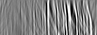
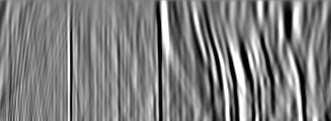
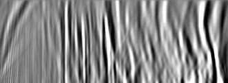
147 CHAPTER 5. 3D FIELD-DATA EXAMPLE 125 Figure 5.10: In-line 3180 of the CAM image with the initial velocity model of Figure 5.5. On the top is the zero-subsurface offset section, and at the bottom ADCIGs. Notice the strong residual moveout on the ADCIGs. The continuous blue line is the top of chalk, and the dashed blue line it the base of chalk. 3dex/. 3dex

148 CHAPTER 5. 3D FIELD-DATA EXAMPLE 126 the gradient computation, as discussed in Chapter 4. As showed in Chapter 2, the CAM-initial conditions can be continuously sampled in the cross-line direction because no cross-line offset is computed, reducing in at least one order of magnitude the number of image-space generalized wavefields to be synthesized. For the base of chalk, we modeled only 30 3D-ISPEW, which are collected at depth 600 m. Using 30 CEES nodes with 8 CPU s each, the modeling takes approximately 10 minutes. A pair of 3D-ISPEW gathers is shown in Figure We expect that crosstalk will be almost completely attenuated during imaging in ISWET, since the number of subsurface offsets computed during ISWET is 25 and the spatial sampling in the x direction is 30 SODCIGs. Velocity optimization A nonlinear conjugate-gradient solver is used for the velocity optimization. Velocity update is constrained to a maximum of 10% variation between iterations. All the wavefield propagation is performed between the depth at which the 30 3D-ISPEW were collected (600 m) and the maximum depth 3300 m. Velocity is updated up to the top of the chalk layer. In 3D, the amplitude variations are more pronounced than in 2D because of the acquisition footprint. To illustrate the amplitude variation problem, we compute the DSO slowness perturbation without applying smoothing, and without extracting the signaled square root from the initial conditions to model 30 pairs of ISPEW (Figure 5.13). In this case, the amplitude variations due to acquisition are even more pronounced. The acquisition footprint is clear, specially around the y-coordinate 4000 m, which is a low fold of coverage region (Figure 5.2). If we extract the signaled square root of the initial conditions for the modeling, or equivalently the signaled fourth root of the gradient, the DSO slowness perturbation presents smaller amplitude variations (Figure 5.14). The gradient of the objective function must be smooth to yield velocity updates

149 CHAPTER 5. 3D FIELD-DATA EXAMPLE 127 Figure 5.11: Slices through the mask operator to select the base of chalk: a) for the zero subsurface offset, and b) for the in-line dex/. 3dex106a

150 CHAPTER 5. 3D FIELD-DATA EXAMPLE 128 Figure 5.12: A pair of 3D source (a) and receiver (b) ISPEW computed for the base of chalk. 3dex/. 3dex109

151 CHAPTER 5. 3D FIELD-DATA EXAMPLE 129 Figure 5.13: DSO slowness perturbation without smoothing and without extracting the signaled square root from the initial conditions for the modeling of 30 pairs of ISPEW. 3dex/. 3dex210

152 CHAPTER 5. 3D FIELD-DATA EXAMPLE 130 Figure 5.14: DSO slowness perturbation without smoothing and extracting the signaled fourth root of the gradient. 3dex/. 3dex211

153 CHAPTER 5. 3D FIELD-DATA EXAMPLE 131 consistent with the Born approximation, as discussed in Chapter 4. We apply a B- spline smoothing with node intervals 420 X 420 X 160 m in the in-line, cross-line and depth directions, respectively. Applying B-spline smoothing on the DSO slowness perturbation of Figure 5.14 mitigates the amplitude variations problems and yields consistent slowness perturbations (Figure 5.15). Figure 5.15: DSO slowness perturbation after B-spline smoothing the DSO slowness perturbation of Figure dex/. 3dex212 Two runs of ISWET were necessary to define the velocity model for the chalk layer. In the first, we used the 30 pairs of ISPEW whose modeling described in the previous subsection. We used two function evaluations in the line search. After seven iterations, optimization stopped due to small variation of the objective function. Figure 5.16 shows the evolution of the objective function. The optimized velocity for

154 CHAPTER 5. 3D FIELD-DATA EXAMPLE 132 Figure 5.16: Evolution of the DSO objective function for the first run of ISWET for the base of chalk. 3dex/. 3dex213 the first run of ISWET is shown in Figure As expected, the migration velocity increased compared to the initial velocity of Figure 5.5. The initial background image and the background image of the seventh iteration can be seen in Figures 5.17 and 5.18, respectively. On the top is the zero subsurface-offset section, and at the bottom are the SODCIGs. Overall, the focusing around the zero-subsurface offset improved. However, close to the salt flanks SODCIGs still show events curving down, indicating velocity inaccuracy. The velocity inaccuracy close to the salt flanks motivated a second run of ISWET for the base of chalk. Again, 30 pairs of ISPEW were modeled, but from initial images limited to approximately 2 km around the salt body. By doing so, we explore the localized nature of these wavefields, as discussed in Chapter 2, so that this second run is targeted for updating the velocity close to the salt flanks. The optimized velocity for the second run of ISWET is shown in Figure Migration velocity further increased compared to the optimized velocity of the first run (Figure 5.19). CAM using this optimized velocity is shown in Figure 5.21, which shows the volume for the zero subsurface offset, and Figure 5.22, which shows the zero subsurface offset on the top, and ADCIGs at the bottom for in-line Compare them with Figures 5.9 and 5.10, respectively. The optimized velocity model allowed imaging of a complex fault system on the right of the salt body, collapsing diffractions from the salt flank, and flattening reflectors in the ADCIGs.

155 CHAPTER 5. 3D FIELD-DATA EXAMPLE 133 Figure 5.17: In-line 3520 of the initial background image of the first run of ISWET for the base of chalk. 3dex/. 3dex214

156 CHAPTER 5. 3D FIELD-DATA EXAMPLE 134 Figure 5.18: In-line 3520 of the background image computed with the optimized velocity model of the first run of ISWET for the base of chalk. 3dex/. 3dex215

157 CHAPTER 5. 3D FIELD-DATA EXAMPLE 135 Figure 5.19: Slices through the optimized velocity from the first run of ISWET for the base of chalk. The dashed white line approximately represents the base of chalk. 3dex/. 3dex216

158 CHAPTER 5. 3D FIELD-DATA EXAMPLE 136 Figure 5.20: Slices through the optimized velocity from the second run of ISWET for the base of chalk. The dashed white line approximately represents the base of chalk. 3dex/. 3dex217

159 CHAPTER 5. 3D FIELD-DATA EXAMPLE 137 Figure 5.21: Slices through the CAM image with the optimized velocity model of Figure Notice the imaging of a big fault close to the salt flank (A), and the focusing of a complex fault system (B, C, and D). 3dex/. 3dex218

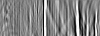
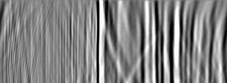
160 CHAPTER 5. 3D FIELD-DATA EXAMPLE 138 Figure 5.22: In-line 3180 of the CAM image with the optimized velocity model of Figure On the top is the zero-subsurface offset section, and at the bottom ADCIGs. Notice flatter reflectors in the ADCIGs compared to those in Figure The continuous blue line is the top of chalk, and the dashed blue line it the base of chalk. 3dex/. 3dex

161 CHAPTER 5. 3D FIELD-DATA EXAMPLE 139 SALT FLOODING Provided that a sufficiently accurate velocity for the chalk layer has been defined, salt flooding was used to delineate the salt body. Top salt was interpreted, and below it velocity was substituted by a constant value of 4500 m/s (Figure 5.23). The picking of top salt is a source of uncertainty for defining the velocity model below, since it is difficult to manually interpret all the high wavenumber components of the irregular top salt. A solution to this problem should be using automatic procedures to identify the top salt (Lomask, 2006; Halpert, 2010). Figure 5.23: Slices through the velocity volume after salt flooding. The dashed white line approximately represents the base of chalk. 3dex/. 3dex311

162 CHAPTER 5. 3D FIELD-DATA EXAMPLE 140 CAM migrated image (Figure 5.24) computed with the velocity of Figure 5.23 supported the interpretation of the base of the salt. As can be seen in Figure 5.24, the lack of a continuous reflector makes the interpretation of the base of salt challenging. Insufficient illumination due to the limited azimuthal coverage and irregular shape of the salt body caused the base of salt to be discontinuous. In this situation, prior geological information would be extremely helpful to constrain interpretation. The lack of it is another source of uncertainty for defining the velocity model below the salt. After interpreting the base of salt, the velocity was edited again (Figure 5.25), so that the salt velocity was confined within the salt body and the initial velocity was inserted below the salt and the chalk layer. With this new velocity model, another run of CAM generated the image (Figure 5.26) from which deeper reflectors are used to model new ISPEW to be used in ISWET for deeper layers. SOLVING FOR SUB-SALT VELOCITIES ACKNOWLEDGMENTS I would like to thank Bob Clapp for making available the common-azimuth migration code and for continuously improving SEP s 3D-interpretation and visualization capability. I am indebted to Dennis Michael, manager of High Productivity Technical Computing (HTPC) initiative hosted by CEES, for his continuous support.

163 CHAPTER 5. 3D FIELD-DATA EXAMPLE 141 Figure 5.24: Slices through the CAM migrated image computed with the salt flooding velocity model of Figure dex/. 3dex312

164 CHAPTER 5. 3D FIELD-DATA EXAMPLE 142 Figure 5.25: Slices through the velocity volume after interpretation of the base of salt. 3dex/. 3dex313

165 CHAPTER 5. 3D FIELD-DATA EXAMPLE 143 Figure 5.26: Slices through the CAM migrated image computed with the velocity model of Figure dex/. 3dex314

166 CHAPTER 5. 3D FIELD-DATA EXAMPLE 144 Figure 5.27: In-line 3180 of the CAM image with the optimized velocity model of Figure On the top is the zero-subsurface offset section, and at the bottom ADCIGs. Notice flatter reflectors in the ADCIGs compared to those in Figure The continuous blue line is the top of chalk, and the dashed blue line it the base of chalk. 3dex/. 3dex