Fast 3D wave-equation migration-velocity analysis using the prestack exploding-reflector model

Transcription

1 Fast 3D wave-equation migration-velocity analysis using the prestack exploding-reflector model Claudio Guerra and Biondo Biondi ABSTRACT In areas of complex geology, velocity-model definition should use methods that describe the complexity of wavefield propagation, such as focusing and defocusing, multipathing, and frequency-dependent velocity sensitivity. Migration-velocity analysis by wavefield extrapolation has the ability to address these issues because it uses wavefields as carriers of information, contrasting with ray-based methods. However, its high cost and low flexibility for parametrizing the model space has prevented its routine industrial use. We overcome those limitations by using new wavefields as carriers of information: the image-space generalized wavefields. These wavefields are synthesized with a pre-stack generalization of the exploding-reflector model. Cost of migration-velocity analysis by wavefield extrapolation is decreased because only a small number of image-space generalized wavefields are necessary to accurately describe the kinematics of velocity errors and because these wavefields can be easily used in a target-oriented way. Flexibility is naturally incorporated because modeling these wavefields have as the initial conditions selected reflectors, which allows using a layer-based parametrization of the model space. Migration with the velocity model optimized by a method that extrapolates image-space generalized wavefields at a very low cost provides good quality and reliable depth images, as we show in a 3D example of the North Sea. INTRODUCTION Migration-velocity analysis (MVA) solves for earth models that explain, under some norm, a residual-moveout parameter measured in the post-migrated domain. Raybased MVA is the most widely used method due its low cost and flexibility to parametrize the model space, which can improve convergence to a geologically reasonable velocity model. However, in the presence of high lateral velocity variation and irregular surfaces, ray-based MVA methods are prone to fail because they do not describe the entire complexity of wavefield propagation. Hence, in those situations it is desirable to use wavefields to define the velocity model. The last decade has seen the development of MVA by wavefield extrapolation (Biondi and Sava, 1999; Sava, 2004; Shen, 2004; Shen and Symes, 2008), which promises to overcome the limitations imposed by the high-frequency approximation

2 Guerra and Biondi WEMVA 2 with the prestack exploding-reflector present in ray methods. MVA by wavefield extrapolation is solved in the image space, using wavefields as carriers of information. Despite its theoretical superiority to ray methods, this relatively new technology has been rarely used in 3D projects (Fei et al., 2009) because of its higher cost and because it is less flexible than its ray-based counterpart in parameterizing the velocity model. We overcome these limitations by using image-space generalized wavefields (Tang et al., 2008a; Guerra et al., 2009; Guerra, 2010). These wavefields are initiated in the image space, having as the initial condition key reflectors selected from a prestack image obtained with a wavefield-extrapolation migration. The image-space generalized wavefields are computed with the pre-stack explodingreflector model (PERM) (Biondi, 2006), which is an extension of the explodingreflector model (Loewenthal et al., 1976). The fundamental idea of PERM is to model downgoing and upgoing wavefields necessary provide a prestack image of a single point on a reflector with same kinematic information as the original prestack image. Synthesizing data sets from a subset of the subsurface has been previously explored by Rietveld and Berkhout (1994) and it further developed into the concept of Common-Focus Point (CFP) technology (Berkhout and Verschuur, 2001; Thorbecke and Berkhout, 2006). CFP technology aims at synthesizing data gathers that contain all the reflections that would have been recorded at the surface if we had placed a point source in the subsurface. A CFP-gather is composed of traces resulting from the time convolution between the shot gather and a focusing operator plus stacking of the stationary phases. The focusing operator is computed by modeling the seismic response of one point at the subsurface. In contrast with CFP, PERM data result from the wave propagation of the prestack image at one point at the subsurface, without operating on the original shot gathers. In this sense, PERM data is more closely related to the CFP operator itself than to the CFP data. To image the entire reflector or group of reflectors, several independent modeling experiments would have to be performed, which could potentially generate data even bigger than the original. However, because of the linearity of wavefield propagation, the modeling experiments can be combined, causing a dramatic data reduction, especially in 3D. When the wavefields are linearly combined after encoding with stochastic phase functions, the image-space phase-encoded wavefields (ISPEW) are generated. Since image-space generalized wavefields are initiated at selected reflectors, a horizonbased strategy to parametrize the velocity model can be naturally incorporated into MVA by wavefield extrapolation. Moreover, these wavefields can be collected at any depth during their propagation, making a target-oriented approach also easily integrated. This paper is organized as follows. First, we describe PERM and how to synthesize the image-space phase-encoded wavefields (ISPEW). Next, we introduce MVA by wavefield extrapolation in the image-space generalized-sources domain, illustrating with the Marmousi model. Finally, we run MVA by wavefield extrapolation, using only 30 pairs of ISPEW, to estimate the 3D-migration-velocity model in the North Sea with the occurrence of a salt body.

3 Guerra and Biondi WEMVA 3 with the prestack exploding-reflector PRESTACK EXPLODING-REFLECTOR MODEL A prestack image computed with an inaccurate velocity model by wavefield-extrapolation methods presents energy departing from the zero subsurface offset. In conventional Born modeling, this entire prestack image is spatially convolved with the source wavefield, generating the receiver wavefield, whose back-propagation and collection at the surface originate data. Source and receiver wavefields must be propagated with the same inaccurate velocity model used in the original migration to preserve the correct kinematics. Now, let us consider the modeling of data necessary to correctly image a single subsurface-offset common-image gather (SODCIG) of a reflector. Since we do not know beforehand which shots contribute to forming the image at a point in the subsurface, we would have to perform several modeling experiments to guarantee illumination similar to that of the original SODCIG. However, ideally, we would like to synthesize a small amount of data with the condition that migration produces the same kinematics of the initial prestack reflector. This is the fundamental idea of the prestack exploding-reflector model (PERM) (Biondi, 2006), whose primary objective is to accelerate migration-velocity analysis. Areal data is generated by PERM, propagating energy of a prestack image. PERM operates in a way similar to the exploding-reflector model (ERM). However, since migration of PERM data can produce a prestack image, PERM can be considered a generalization of ERM. The modeling of PERM wavefields can be carried out by any wavefield-continuation scheme. Here, we use the following one-way wave equations: { ( ) i ω z 2 s 2 0(x) k 2 D(x, ω; x m ) = I D (x m, h), (1) D(x, y, z = z max, ω; x m ) = 0 and { ( ) + i ω z 2 s 2 0(x) k 2 U(x, ω; x m ) = I U (x m, h) U(x, y, z = z max, ω; x m ) = 0, (2) where ω is the radial frequency, s 0 is the same background velocity used to produce the initial prestack image, D and U represent the downgoing and the upgoing PERM wavefields, respectively, I D and I U are subsets of the prestack image centered at x m for a single reflector, suitable for the initial conditions for modeling downgoing and upwgoing PERM wavefields, respectively. The information along the subsurfaceoffset h dimension of the initial conditions is projected onto the x dimension for the modeling. The subsurface offset is parameterized as h = (h x, h y ), where h x and h y are the inline- and the crossline-subsurface offsets, respectively. Notice that if the prestack image has energy focused at zero subsurface offset, the initial conditions can be parameterized only by its spatial coordinates, and PERM is equivalent to ERM. The initial conditions are obtained by rotating the original unfocused SODCIGs according to the apparent geological dip of the reflector. This operation corrects for the image-point dispersal due to velocity inaccuracy, causing events with different

4 Guerra and Biondi WEMVA 4 with the prestack exploding-reflector reflection angles from the same reflection point to be imaged at different locations. This is a consequence of not shifting the wavefields along the apparent geological-dip direction (Biondi and Symes, 2004) when applying the multi-offset image condition (Rickett and Sava, 2002). The 2D geometry that explains the rotation is depicted in Figure 1 for the cases of migration velocity which is slower (Figure 1a) and faster (Figure 1b) than the correct one. Figure 1: Geometry for the computation of SODCIGs. Source, receiver and image points are labeled with S, R and I, respectively. The subscript hx corresponds to subsurface offsets computed with horizontal shift. The subscript hg corresponds to subsurface offsets computed by shifting along the apparent geological dip α. a) Underestimated velocity, and b) overestimated velocity. Modified from Biondi and Symes (2004). The angles γ + α and γ α are the source and receiver ray angles, respectively. They are the propagation directions of the wavefields locally at the image point. In 2D, α and γ are related to slopes in the pre-stack image according to tan α = dz m dx m (3) tan γ = dz dh x, (4) where the subscript m in equation 3 refers to the local nature of the relationship. The solutions of the differential equations 3 and 4 define slant-stack paths, which allow us to transform the 2D pre-stack image I(x, z, h x ) into I(x, z, α, γ). To align the initial conditions with the geological dip, the dip along the subsurface-offset axis is changed, yielding the new subsurface offset h xd and h xu for the initial conditions of the modeling of downgoing and upgoing PERM wavefields, respectively. This is accomplished by solving the following differential equations: tan(γ + α) = dz d h, (5) xd

5 Guerra and Biondi WEMVA 5 with the prestack exploding-reflector tan(γ α) = dz d h xu. (6) The solutions of equations 5 and 6 define new slant-stack operations, which reduce the dimensionality of the decomposed pre-stack image by transforming I(x, z, α, γ) into I D (x, z, h xd ) and I U (x, z, h xu ). In 3D, the cross-line subsurface offsets also must be rotated. A complete description of the 3D rotation is given by Guerra (2010). PERM as described by equations 1 and 2 generates sufficient data to image a single SODCIG. However, to fully image a reflector, we would have to model data that could potentially be even greater than the original data. Using the linearity of wavefield propagation, the modeling experiments can be combined in a way that PERM data size is decreased. Hence, a group of equally spaced SODCIGs is simultaneously injected into the modeling according to { ( ) i ω z 2 s 2 0(x) k 2 D(x, ω) = Î D (x h), (7) D(x, y, z = z max, ω) = 0 and { ( ) + i ω z 2 s 2 0(x) k 2 Û(x, ω) = Î U (x + h) Û(x, y, z = z max, ω) = 0, (8) where ÎD and ÎU are the combination of SODCIGs for a single reflector to be used as the initial conditions for the modeling of combined downgoing and upgoing wavefields, D and Û, respectively. The selection of SODCIGs can be thought of as the multiplication of the pre-stack image by a 2D comb function, which is shifted laterally to select new set of SODCIGs to initiate the modeling of another pair of combined wavefields. After shifting along one period of the sampling function in the x and y directions, all the points on the reflector are used in the modeling. Consequently, the number of modeling experiments equals the number of lateral shifts of the sampling function. Depending on the spatial periods of the sampling function, crosstalk between wavefields modeled from different SODCIGs occurs during migration. If the periods of the 2D comb function are chosen to be the decorrelation distances of twice the x and y subsurface-offset range, no crosstalk is generated. If more than one reflector is used, each reflector must be separately injected into the modeling, so that wavefields from different reflectors do not cross-correlate during imaging, avoiding reflector crosstalk. These procedures to avoid crosstalk limit data size reduction with PERM. To overcome this limitation, two different strategies can be used. One strategy mitigates the reflector crosstalk, benefiting from the fact that the image of a reflector is formed at the zero time of wavefield propagation when the migration velocity is accurate. When migration velocity is inaccurate, focusing of the image departs from the zero time. This can be potentially used to update the velocity model (Sava and Fomel, 2006; Yang and Sava, 2009). Depending on the magnitude of the velocity errors and the distance between reflectors, selecting events

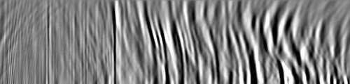
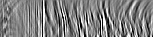
6 Guerra and Biondi WEMVA 6 with the prestack exploding-reflector with propagation time close to zero can avoid cross-correlating unrelated events. This is the principle of the time-windowed imaging condition, which for a single pair of PERM wavefields reads I W(x, h) = [ ] ] F 1 D (x h) F [Û(x 1 + h), (9) tw 2 t tw 2 where t w is the length of the time window. When using one-way propagators, the wavefields are inverse Fourier transformed to time by F 1. Another strategy is to phase-encode the modeling experiments. Phase-encoding is a well stablished technique for decreasing the cost of seismic imaging by linearly combining the shot records (Schultz and Claerbout, 1978; Whitmore, 1995; Romero et al., 2000; Sun et al., 2002; Liu et al., 2006; Duquet and Lailly, 2006).In general, phase-encoding is usually performed in the data space. PERM wavefields can be phase-encoded in the image space, using stochastic phase functions parametrized according to the model-space coordinates and selected reflector. Phase-encoding the modeling experiments mitigates not only crosstalk between wavefields modeled from different reflectors as well as crosstalk between wavefields modeled from different SODCIGs. This is achieved by phase-encoding the initial conditions Ĩ, according to: Ĩ( x, h, q, ω) = δ( x m x)β( x, j, q, ω)w j ( x, h)i( x, h), (10) m j where W j selects the reflector j by identifying and windowing it in the pre-stack image I, and β( x, j, q, ω) is a pseudo-random phase-encoding function defined as β( x, j, q, ω) = e iɛ(bx,j,q,ω), (11) with ɛ( x, j, q, ω) usually being a uniformly distributed pseudo-random sequence with zero mean. Sequences used in third- and fourth-generation cellphones can also be used to phase-encode the modeling (Guerra and Biondi, 2008). Downgoing and upgoing image-space phase-encoded wavefields (ISPEW) initiated at the same SODCIG and from the same reflector are equally encoded, whereas downgoing and upgoing ISPEW initiated at different SODCIGs and from the different reflectors have different codes assigned to them. According to the law of large numbers, crosstalk attenuation is more effective for more random realizations. PERM wavefields can be collected at any depth, which can be the top of a region of inaccurate velocity, having key reflectors within this region as the initial conditions. By doing so, velocity update will be restricted to the inaccurate velocity region. The use of key reflectors characterizes a target-oriented strategy to perform MVA by wavefield extrapolation. These two features along with the decrease of data size yielded by PERM drastically decreases the cost of MVA by wavefield extrapolation. To illustrate the computation of PERM data and ISPEW, a prestack image computed with the inaccurate velocity model of Figure 2b is used as the initial conditions

7 Guerra and Biondi WEMVA 7 with the prestack exploding-reflector after rotation according to the apparent geological dip. Data comprise 375 splitspread shots, with 6000 m maximum offset, computed by one-way Born modeling using the smooth Marmousi velocity model of Figure 2a along with the reflectivity derived from the true Marmousi model. The inaccurate velocity model is exactly the same as the correct velocity model up to the black horizon. From this horizon down, velocity is strongly smoothed and multiplied by 0.9. The curvature of the reflectors in the SODCIG and the pull-up of reflectors in the center of Figure 3a reflect the velocity inaccuracy. We use the four reflectors shown in Figure 3b to model 35 pairs of PERM data (Figure 4) and 11 pairs of ISPEW (Figure 5). Migration of the 35 pairs of PERM data using the conventional imaging condition is shown in Figure 6a and using the time-windowed-imaging condition is shown in Figure 6b. Notice that this modified imaging condition almost completely avoids reflector crosstalk. Migration of the 11 pairs of ISPEW is shown in Figure 7. Reflectors are satisfactorily imaged and crosstalk is dispersed throughout the image. Figure 2: Edited velocity models for the Marmousi example: a) Smooth velocity model used to model the Born data. b) Background velocity model used to migrate the Born data, and to model and migrate PERM data. Residual-moveout panels from images computed with the original shot records (Figure 8a), with 35 pairs of PERM data (Figure 8b), and with 11 ISPEW (Figure 8c) are used to analyze the quality of the moveout information. Notice that in the ADCIGs corresponding to images computed with PERM wavefields and ISPEWs, less

8 Guerra and Biondi WEMVA 8 with the prestack exploding-reflector Figure 3: a) Pre-stack image computed with the background velocity model. b) Selected reflectors from the background image to perform modeling of wavefields. Figure 4: PERM wavefields for the Marmousi example: a) Upward wavefield. b) Downward wavefield.

9 Guerra and Biondi WEMVA 9 with the prestack exploding-reflector Figure 5: ISPEW for the Marmousi example: a) Upward wavefield. b) Downward wavefield. Figure 6: Pre-stack image computed with PERM wavefields and background velocity model using: a) the conventional imaging condition (equation??), and b) the time-windowed imaging condition (equation 9). Reflector crosstalk is avoided when reflectors are sufficiently separated. However, some residual crosstalk is still present (RC). Notice the phase difference of the PERM image due to the squaring of the wavelet when compared to the windowed reflectors of Figure 3b.

10 Guerra and Biondi WEMVA 10 with the prestack exploding-reflector Figure 7: Pre-stack images computed with: a) Four random realizations of ISPEWs, and b) a single random realization.

11 Guerra and Biondi WEMVA 11 with the prestack exploding-reflector events are present since only four reflectors were selected to model these wavefields. The corresponding reflectors in the original shot-profile image are highlighted by the green boxes in Figure 8a. The residual moveout information in the four panels is very similar. However, some crosstalk not entirely rejected by the time-windowed imaging condition causes the residual-moveout information lose resolution in Figure 8b when compared to Figure 8c. Figure 8: ADCIGs (top) and ρ-panels (bottom) corresponding to images computed by: a) Shot-profile migration of 360 shot gathers, b) areal-shot migration of 35 PERM wavefields using the time-windowed imaging condition, c) areal-shot migration of 44 ISPEWs corresponding to four random realizations, and d) areal-shot migration of 11 ISPEWs corresponding to a single random realization. The moveout information is basically the same. The cost for obtaining the images in Figure 8 widely varies. For instance, migrating 11 ISPEW is approximately 30 times faster than migrating all the 375 original shots. Using the same wavefields, computing the gradient of the objective function of MVA by wavefield-extrapolation can be 60 times faster. This difference in performance is even more dramatic when we consider that several iterations of migrations and gradient computations are performed during migration-velocity optimization by wavefield-extrapolation. MVA BY WAVEFIELD-EXTRAPOLATION Optimization of the migration velocity is a non-linear inverse problem. When using wavefield-extrapolation methods, it searches for an optimal background velocity which minimizes an objective function defined in the image space. The residual that

12 Guerra and Biondi WEMVA 12 with the prestack exploding-reflector characterizes the objective function is represented by the perturbed image Î, which, in turn, is derived from the background image Î0 computed with the background slowness s 0. The perturbed image can be computed by the linearized-residual prestack-depth migration (Sava, 2003), and it is used in the wave-equation migration-velocity analysis (Biondi and Sava, 1999; Sava, 2004). Also, the perturbed image can be computed by the differential-semblance-optimization (DSO) operator (Symes and Carazzone, 1991), and it is used in the differential-semblance velocity optimization (DSVA) (Shen, 2004; Shen and Symes, 2008). Under the l 2 norm, the DSVA objective function J DSO is J DSO = 1 2 Î 2 = 1 2 H[Î0] 2, (12) where H is the DSO operator either in the subsurface-offset domain or in the angle domain. In the subsurface-offset domain, DSO penalizes energy at zero offset, by weighting the background image with the absolute value of the subsurface offset. In the angle domain, DSO penalizes flattening of events, by taking the derivative of the background image along the aperture angle. Gradient-based optimization techniques, such as the nonlinear conjugate-gradient method, can be used in the optimization, to which the gradient must be explicitly computed. The gradient J DSO of the objective function of equation 12 with respect to the slowness s is J DSO = T H HI 0, (13) where T = I s s=s0 is the wave-equation tomographic operator (WETOM), evaluated at s = s 0, which is composed of several operators and linearly maps the slowness perturbation s into the perturbed image. WETOM has been evaluated in the source and receiver domain (Sava, 2004), in the shot-profile domain (Shen, 2004), and in the generalized-sources domain both in the data and in the image space (Tang et al., 2008b). We discuss WETOM in the image-space generalized-sources domain, using 35 ISPEW modeled from 12 reflectors (Figure 9) selected from the background image computed with the velocity model of Figure 10b. This velocity model is obtained by smoothing the Marmousi velocity model (Figure 10a) and multiplying it by 0.9 only below the black horizon. In the areal-shot migration of image-space generalized wavefields, wavefields are downward continued with the following one-way wave equations: { ( ) + i ω z 2 s 2 (x) k 2 D(x, p, ω) = 0 D(x, y, z = z min, p, ω) = D(x, y, z = z min, p, ω), (14) and { ( ) i ω z 2 s 2 (x) k 2 Û(x, p, ω) = 0 Û(x, y, z = z min, p, ω) = Ũ(x, y, z = z min, p, ω), (15)

13 Guerra and Biondi WEMVA 13 with the prestack exploding-reflector Figure 9: Selected reflectors used to model 35 pairs of ISPEW. Figure 10: Velocity models used in the explanation of MVA by wavefield extrapolation using the image-space generalized wavefields: a) True Marmousi velocity model. b) Background velocity model used in the initial migration and in the modeling of ISPEW.

14 Guerra and Biondi WEMVA 14 with the prestack exploding-reflector where D(x, p, ω) is the image-space generalized downgoing wavefield for a single frequency, Û(x, p, ω) is the image-space generalized upgoing wavefield for a single frequency; p is the index of the areal shot, and D(x, y, z = z min, p, ω) and Ũ(x, y, z = z min, p, ω) are the data synthesized with PERM using phase encoding or not, and collected at z = z min, which denotes the top of a target zone. PERM data serve as the boundary conditions of equations 14 and 15, respectively. Snapshots of the background ISPEW are shown in Figure 11. Figure 11: Snapshots of kground ISPEW: a) downgoing, and b) upgoing wavefields. The cross-correlation imaging condition produces the image Î(x, h) (Figure 12) Î(x, h) = D (x h, p, ω)û(x + h, p, ω). (16) p ω The perturbed image is derived by applying the product rule to equation 16, which gives Î(x, h) = D (x h, p, ω)û0(x + h, p, ω) + p ω D 0(x h, p, ω) Û(x + h, p, ω), (17) where D 0 (x h, p, ω) and Û0(x + h, p, ω) are the image-space generalized background downgoing and upgoing wavefields computed with the background slowness; and D(x h, p, ω) and Û(x + h, p, ω) are the image-space generalized perturbed

15 Guerra and Biondi WEMVA 15 with the prestack exploding-reflector Figure 12: Background image computed with the image-space generalized background wavefields of Figure 11. downgoing wavefield and the image-space generalized perturbed upgoing wavefield, respectively. These image-space generalized perturbed wavefields are the response to a slowness perturbation. The image-space generalized perturbed wavefields satisfy the following one-way wave equations linearized with respect to the slowness: { ( ) + i ω z 2 s 2 0(x) k 2 D(x, p, ω) = D SC (x, p, ω) D(x,, (18) y, z = z min, p, ω) = 0 and { ( ) + i ω z 2 s 2 0(x) k 2 Û(x, p, ω) = ÛSC(x, p, ω) Û(x, y, z = z min, p, ω) = 0. (19) Snapshots of the image-space generalized perturbed wavefields are shown in Figure 13. No scattering occurs at depth levels shallower than z min because the initial conditions above this minimum depth are null. The wavefields in the right-hand side of equations 18 and 19 are the image-space generalized scattered downgoing and upgoing wavefields, respectively, which result from the interaction of the image-space generalized background wavefields with a slowness perturbation according to D SC (x, p, ω) = iω s(x) 1 k 2 ω 2 s 2 0 (x) D0 (x, p, ω) (20)

16 Guerra and Biondi WEMVA 16 with the prestack exploding-reflector Figure 13: Snapshots of image-space generalized perturbed wavefields: a) source, and b) receiver. and Û SC (x, p, ω) = iω s(x) 1 k 2 ω 2 s 2 0 (x) Û 0 (x, p, ω). (21) These wavefields are injected at every depth level during the recursive downward propagation of the perturbed wavefields. The image-space generalized perturbed source and receiver wavefields are used along with the precomputed image-space generalized background source and receiver wavefields in equation 17 to generate the perturbed image (Figure 14). The adjoint WETOM T is obtained by the folowing operations. First, the adjointimaging condition is applied to compute the image-space generalized perturbed downgoing and upgoing wavefields according to the following convolutions: D(x, p, ω) = h Û(x, p, ω) = h Î(x, h)û0(x + h, p, ω) Î(x, h) D 0 (x h, p, ω). (22) The image-space generalized perturbed wavefields are upward propagated using the adjoint counterparts of equations 18 and 19. At every depth of their upward propagation, the image-space generalized perturbed downgoing wavefield is cross-correlated

17 Guerra and Biondi WEMVA 17 with the prestack exploding-reflector Figure 14: Perturbed image computed with equation 17. with the image-space generalized scattered downgoing wavefield, and the image-space generalized perturbed upgoing wavefield is cross-correlated with the image-space generalized scattered upgoing wavefield to generate the slowness perturbation according to ŝ(x) = D SC(x, p, ω) D(x, p, ω) + p ω ÛSC(x, p, ω) Û(x, p, ω). (23) The slowness perturbation for the Marmousi example computed in the image-space generalized sources domain using ISPEWs is shown in Figure 15. When performing velocity optimization using DSVA, for instance, the perturbed image in equation 22 is computed with DSO at the begining of every nonlinear iteration. DSO easily automates migration-velocity optimization. However, neither the phase nor the amplitudes of the DSO perturbed image are consistent with those of the perturbed image computed by the forward one-way WETOM. These differences prevent the use of linear conjugate-gradient methods, and therefore the objective function computed with DSO is typically minimized by nonlinear optimization methods. The gradient of the wave-equation tomography objective function is sensitive to amplitude variations of the prestack image caused by uneven illumination. Since these amplitude variations are not related to velocity inaccuracy, we should ideally attenuate them using some sort of illumination compensation scheme (Valenciano

18 Guerra and Biondi WEMVA 18 with the prestack exploding-reflector Figure 15: Slowness perturbation from back-projected image perturbations computed with 35 ISPEWs. et al., 2009; Tang, 2009). Instead, to prevent these amplitude variations we apply a B-spline smoothing to the gradient, which consists of representing the gradient as B-spline basis functions, using the adjoint operator B, and transforming it back to the Cartesian space, using the forward operator B. When using image-space generalized wavefields, a target-oriented strategy can be adopted if the velocity model is sufficiently accurate for shallower layers. A mask operator M is applied to the gradient, zeroing out amplitudes in the accurate velocity region, preventing the velocity model from being updated. Since the gradient is not properly scaled, we normalize it by the inverse of its maximum absolute value multiplied by the minimum slowness, which characterizes the diagonal operator F. To improve and sometimes guarantee convergence, we would like to limit the velocity update from one iteration with respect to its previous values. In other words, we would like the new velocity to vary within a range defined by a percentage of the velocity from the previous iteration. This can be implemented by applying to the gradient either a nonlinear (since it depends on the velocity) diagonal operator, or a diagonal operator W linearized around the initial velocity. Therefore, in contrast with the gradient of equation 13, the one we use to update the velocity model is J DSO = WFMBB T s=s0 H H Ĩ. (24) s=s0 3D EXAMPLE We estimate the migration-velocity model with 3D ISPEW synthesized from prestack images of the North Sea. The challenges for defining the velocity model for this dataset are due to a possibly irregular salt body, the intense faulting, the amplitude variations caused by irregular acquisition, the short source-receiver offsets, and the

19 Guerra and Biondi WEMVA 19 with the prestack exploding-reflector limited source-receiver azimuths. Because of the narrow azimuthal configuration, the 3D dataset was submitted to azimuth-moveout (AMO), and common-azimuth migration (CAM) images are used as the initial conditions for the modeling of very few 3D ISPEW. All the computations were carried out on computer nodes of the Stanford Center for Computational Earth & Environmental Science (CEES). Thirty nodes of Dual Nehalem 5520 with 24Gb RAM were used, accounting to 240 CPUs. To generate 30 pairs of 3D ISPEWs, using 196 frequencies, it took 10 minutes. On average, each iteration of the velocity optimization, consisting of one function evaluation, the gradient computation, and two additional function evaluations for the line search, took approximately two hours. The 3D North Sea dataset spans over an area of approximately 55 km 2, with 13.5 km in-lines and 4 km cross-lines. It was acquired using dual sources at intervals of 25 m in the in-line direction and 50 m in the cross-line direction, with three cables 100 m apart and a maximum offset 3600 m. The limited cross-line offsets resulting from this acquisition configuration impose limitations in the azimuthal distribution. The offset distribution is spatially quite irregular, as can be seen in the fold of coverage maps for different offset ranges (Figure 16). The acquisition footprint is evident, with a wide low-fold region occurring for in-lines around 4000 m in the y direction. In spite of the regularization provided by AMO, amplitude variations caused by the offset irregularity still persists as can be seen in Figure 17. It shows time slices at 2.8 s through the trace envelope for different offset cubes taken from the regularized data. Figure 16: Fold of coverage plots: a) full offset, b) m offset, c) m offset, and d) m offset. Even though the fold irregularity (Figure 16) and amplitude imbalance (Figure 17) are in the data-space, we will see that they will be evident in the amplitudes of the gradient of the objective function at approximately the same spatial position.

20 Guerra and Biondi WEMVA 20 with the prestack exploding-reflector Figure 17: Time slices through the trace envelope for different offset cubes from the regularized data: a) offset 200m, b) offset 1200 m, c) offset 2400 m, and d) offset 3000 m. The velocity model provided along with the data (Figure 18), herein called the original velocity model, presents a general layered structure with an overhanging salt dome connected to a deeper layer with the same velocity as that of the salt dome. The shallower layer with a domed structure is a reflection-free chalk layer, herein called chalk layer. The final velocity model we derive shows remarkable differences when compared to the original velocity model, especially in the salt body shape. To derive the initial velocity model, the sediment velocity above the chalk layer was refined using residual prestack depth-migration scans. Below the top of chalk, velocity was heavily smoothed using a 5000 m wide 2D median smoother. In addition, to increase the inaccuracy of the initial velocity model, velocity was scaled down by a factor of 0.9 (Figure 19). A layer-stripping approach was used to define the velocity for the chalk layer, considering a sufficiently accurate velocity for the sediments above. Then, the top salt was interpreted, and a salt flooding procedure enabled the interpretation of the base of salt. The interpretation of the base of salt can be considered the main source of uncertainty of this example, since no previous geological information was available. Finally, a group of reflectors below the salt is used to define the velocity structure for the deeper part. The initial velocity model produces the CAM image of Figure 20, which shows the volume for the zero subsurface offset, and Figure 21, which shows the zero subsurface offset on the left, and ADCIGs on the right for in-line The effects of migrating with a too low velocity are evidenced by poorly collapsed diffractions close to the salt flank, poorly imaged faults, and reflectors curving up in the ADCIGs. The base of chalk was interpreted in the 3D pre-stack volume and used as input

21 Guerra and Biondi WEMVA 21 with the prestack exploding-reflector Figure 18: Slices through the original velocity model.

22 Guerra and Biondi WEMVA 22 with the prestack exploding-reflector Figure 19: Slices through the initial velocity model used in the velocity optimization.

23 Guerra and Biondi WEMVA 23 with the prestack exploding-reflector Figure 20: Slices through the CAM image with the initial velocity model of Figure 19. Notice poorly collapsed diffractions close to the salt flank (A and D), and poorly imaged faults (B and C) caused by migrating with an inaccurate velocity.

24 Guerra and Biondi WEMVA 24 with the prestack exploding-reflector Figure 21: In-line 3180 of the CAM image with the initial velocity model of Figure 19. On the left is the zero-subsurface offset section, and on the right ADCIGs. Notice the strong residual moveout on the ADCIGs. The continuous blue line is the top of chalk, and the dashed blue line it the base of chalk.

25 Guerra and Biondi WEMVA 25 with the prestack exploding-reflector for the modeling of 30 ISPEW. In-line and cross-line intervals of the CAM image were interpolated from 20 m to 30 m, which are the in-line and cross-line intervals used for optimizing the migration velocity. Since no cross-line offset is computed, the CAM initial conditions can be continuously sampled in the cross-line direction, reducing by at least one order of magnitude the number of image-space generalized wavefields to be synthesized. For the base of chalk, only 30 3D ISPEWs were modeled and collected at 600 m depth. A pair of 3D-ISPEW is shown in Figure 22. Since the number of subsurface offsets that will be used during ISWET is 25 and the spatial sampling in the x direction of 30 SODCIGs is used to model the 3D ISPEWs, crosstalk is expected to be strongly attenuated during imaging in ISWET. In the velocity optimization for the chalk layer, velocity update is constrained to a maximum of 10% variation between iterations. All the wavefield propagation is performed between the depth at which the 30 3D ISPEWs were collected (600 m) and the maximum depth (3300 m). Velocity is updated up to the top of the chalk layer. To illustrate the amplitude variation problem, we compute the slowness perturbation without applying smoothing (Figure 23). The acquisition footprint is clear, specially around the y coordinate 4000 m, which is a region with low-fold of coverage (Figure 16). The gradient of the objective function must be smooth to yield velocity updates consistent with the Born approximation. We apply a B-spline smoothing with node intervals of 420 X 420 X 160 m in the in-line, cross-line and depth directions, respectively. Applying B-spline smoothing on the DSO slowness perturbation of Figure?? mitigates the amplitude-variation problems and yields consistent slowness perturbations (Figure 24). Two runs of velocity optimization were necessary to define the velocity model for the chalk layer. The first used wavefields modeled from all the extension of base of chalk. Since CAM with the resulting velocity revealed velocity inaccuracy close to the salt flanks, new ISPEWs were modeled having the initial conditions limited to approximately 2 km around the salt body. By doing this, we explore the localized nature of these wavefields, so that this second run is targeted for updating velocity close to salt flanks. In both runs, two function evaluations were used in the line search. Figure 25 shows the evolution of the objective function for the first run. The optimized velocity for the first run of ISWET is shown in Figure 28. The initial background image and the background image of the seventh iteration can be seen in Figures 26 and 27, respectively. On the left is the zero-subsurface-offset section, and on the right are the SODCIGs. Overall, the focusing around the zero subsurface offset improved. However, close to the salt flanks, SODCIGs still show events curving down. The optimized velocity for the second run of ISWET is shown in Figure 29. CAM using this optimized velocity is shown in Figure 30, which shows the volume for the zero subsurface offset, and Figure 31, which shows the zero subsurface offset on the

26 Guerra and Biondi WEMVA 26 with the prestack exploding-reflector Figure 22: A pair of 3D source (a) and receiver (b) ISPEWs computed for the base of chalk.

27 Guerra and Biondi WEMVA 27 with the prestack exploding-reflector Figure 23: Slowness perturbation without smoothing.

28 Guerra and Biondi WEMVA 28 with the prestack exploding-reflector Figure 24: Slowness perturbation after B-spline smoothing the slowness perturbation of Figure??.

29 Guerra and Biondi WEMVA 29 with the prestack exploding-reflector Figure 25: Evolution of the DVSA objective function for the first run of ISWET for the base of chalk. top, and ADCIGs at the bottom for in-line Compare these figures with Figures 20 and 21, respectively. The optimized velocity model allowed imaging of a complex fault system on the right of the salt body, collapsing diffractions from the salt flank, and flattening reflectors in the ADCIGs. Once a sufficiently accurate velocity for the chalk layer had been defined, salt flooding was used to delineate the salt body. The top salt was interpreted, and below it velocity was replaced by a constant value of 4500 m/s. CAM image computed with the salt-flooded velocity supported the interpretation of the base of the salt. Insufficient illumination due to the limited azimuthal coverage and irregular shape of the salt body caused the base of salt to be discontinuous. In this situation, prior geological information would be extremely helpful to constrain the interpretation. The lack thereof is a source of uncertainty for defining the velocity model below the salt. After the base of salt was interpreted, salt velocity was delineated and the initial velocity was inserted below the salt and the chalk layer. This new velocity model produced the CAM image in Figure 33 from which deeper reflectors are used to model new ISPEWs to optimize sub-salt and sub-chalk velocity. Seven reflectors were interpreted (Figure 35) and used as the initial conditions for the modeling of 30 3D ISPEWs. These wavefields were collected at a depth of 1650 m, which is the minimum depth used in the velocity optimization. The maximum depth is 4800 m.

30 Guerra and Biondi WEMVA 30 with the prestack exploding-reflector Figure 26: In-line 3520 of the initial background image of the first run of ISWET for the base of chalk.

31 Guerra and Biondi WEMVA 31 with the prestack exploding-reflector Figure 27: In-line 3520 of the background image computed with the optimized velocity model of the first run of ISWET for the base of chalk.

32 Guerra and Biondi WEMVA 32 with the prestack exploding-reflector Figure 28: Slices through the optimized velocity from the first run of ISWET for the base of chalk. The dashed white line approximately represents the base of chalk.

33 Guerra and Biondi WEMVA 33 with the prestack exploding-reflector Figure 29: Slices through the optimized velocity from the second run of ISWET for the base of chalk. The dashed white line approximately represents the base of chalk.

34 Guerra and Biondi WEMVA 34 with the prestack exploding-reflector Figure 30: Slices through the CAM image with the optimized velocity model of Figure 29. Notice the imaging of a big fault close to the salt flank (A), and the focusing of a complex fault system (B, C, and D).

35 Guerra and Biondi WEMVA 35 with the prestack exploding-reflector Figure 31: In-line 3180 of the CAM image with the optimized velocity model of Figure 29. On the left is the zero-subsurface offset section, and on the right ADCIGs. Notice flatter reflectors in the ADCIGs compared to those in Figure 21. The continuous blue line is the top of chalk, and the dashed blue line it the base of chalk.

36 Guerra and Biondi WEMVA 36 with the prestack exploding-reflector Figure 32: Slices through the velocity volume after interpretation of the base of salt.

37 Guerra and Biondi WEMVA 37 with the prestack exploding-reflector Figure 33: Slices through the CAM migrated image computed with the velocity model of Figure 32.

38 Guerra and Biondi WEMVA 38 with the prestack exploding-reflector Figure 34: Slices through the prestack image computed with the migration velocity of Figure 32: a) the zero subsurface offset, and b) the in-line 3520.

39 Guerra and Biondi WEMVA 39 with the prestack exploding-reflector Figure 35: Slices through the windowed prestack image, showing the selected reflectors for the modeling of 30 3D ISPEWs to be used in the sub-salt velocity optimization: a) the zero subsurface offset, and b) the in-line 3520.

40 Guerra and Biondi WEMVA 40 with the prestack exploding-reflector In the sub-salt velocity optimization, the intervals between B-spline nodes is 1050 m in the x and y directions and 150 m in the z direction. A maximum of 5% local velocity variation is allowed between iterations, and two function evaluations are performed in the line search. The evolution of the objective function normalized by its initial value is shown in Figure 36. The final objective function dropped 10%. This decrease is small compared to the 40% decrease for the velocity optimization of the chalk layer. Apart from the poorer illumination in the sub-salt and sub-chalk case, which prevents the complete focusing at the zero subsurface offset, this difference can be explained by the different levels of crosstalk. For the chalk layer, only crosstalk from different SODCIGs occurs, whereas for the sub-salt case, crosstalk from different SODCIGs and reflector crosstalk were generated. Figure 36: Evolution of the DVSA objective function of the sub-salt velocity optimization. CAM with the optimized velocity model can be seen in Figure 37. For comparison, CAM with the initial velocity model and CAM with the original velocity model are shown in Figures 38 and 39. When compared with the results using the initial velocity model, the improvements obtained with the optimized velocity model are clear: flatter angle gathers, better focusing of the reflectors, and imaging of the faults. The improvements compared to the original (unmodified) velocity model are also clear: better focusing of reflectors and slightly flatter angle gathers below the salt as well as close to its flanks. Comparisons between the CAM images obtained with the initial, with the original, and with the final velocity models, for different in-lines and cross-lines are shown in Figures 40, 41, and 42. The images are displayed as vertical slices through the migrated cube and show the zero subsurface offset. The left panel of each figure shows the in-line, and the right panel shows the cross-line. Ovals highlight the main differences. Overall, the final images present better quality than do the initial and original images, expressed by better focusing and continuity of reflectors in the chalk layer as well as in the sub-salt region.

41 Guerra and Biondi WEMVA 41 with the prestack exploding-reflector Figure 37: In-line 4060 of the CAM image with the final velocity model after optimization for the chalk layer, salt flooding, and sub-salt velocity optimization. On the top is the zero-subsurface offset section, and at the bottom ADCIGs.

42 Guerra and Biondi WEMVA 42 with the prestack exploding-reflector Figure 38: In-line 4060 of the CAM image with the initial velocity model. On the top is the zero-subsurface offset section, and at the bottom ADCIGs.

43 Guerra and Biondi WEMVA 43 with the prestack exploding-reflector Figure 39: In-line 4060 of the CAM image with the original velocity model. On the top is the zero-subsurface offset section, and at the bottom ADCIGs.

44 Guerra and Biondi WEMVA 44 with the prestack exploding-reflector Figure 40: On the left panel is the in-line 3320 and on the right panel is the cross-line 5220 of the CAM images obtained with: a) the initial velocity model, b) the original velocity model, and c)the final velocity model after optimization for the chalk layer, salt flooding, and sub-salt velocity optimization. The oval in the in-line of the final image show better focusing and continuity for the sub-salt reflectors as well as for the salt flank. Besides focusing and continuity, the oval in the cross-line of the final image show unstructured sub-salt reflectors not pulled up by velocity errors.

45 Guerra and Biondi WEMVA 45 with the prestack exploding-reflector Figure 41: On the left panel is the in-line 3680 and on the right panel is the cross-line 6880 of the CAM images obtained with: a) the initial velocity model, b) the original velocity model, and c)the final velocity model after optimization for the chalk layer, salt flooding, and sub-salt velocity optimization. The oval in the in-line of the final image show better focusing and continuity for the sub-salt reflectors. Besides focusing and continuity, the oval in the cross-line of the final image show unstructured sub-salt reflectors not pulled up by velocity errors.

46 Guerra and Biondi WEMVA 46 with the prestack exploding-reflector Figure 42: On the left panel is the in-line 4060 and on the right panel is the cross-line 9400 of the CAM images obtained with: a) the initial velocity model, b) the original velocity model, and c)the final velocity model after optimization for the chalk layer, salt flooding, and sub-salt velocity optimization. The oval in the in-line of the final image show better focusing and continuity for the sub-salt reflectors. In the crossline, the upper oval of the final image show better definition of subtle faults in the chalk layer, the lower oval highlights better continuity of the reflectors, and the arrow labeled F indicates better fault imaging not clear in the initial and original images.

47 Guerra and Biondi WEMVA 47 with the prestack exploding-reflector CONCLUSIONS Using 3D ISPEWs has proved to greatly accelerate 3D-MVA by wavefield extrapolation, due to the small number of wavefields needed to satisfactorily describe the kinematics of the prestack image and the fact that they are computed in a target-oriented manner. These synthesized wavefields made it possible to solve for the 3D-migration velocity with limited computational resources. Considering the computational resources available in the industry, using 3D ISPEWs can turn MVA by wavefield extrapolation an interactive process, which can yield more reliable solutions. Solving for migration velocity in a target-oriented manner with wave-equation methods allows updating the velocity model not only within a limited depth range, but also within a limited lateral extent. This is achieved by selecting a specific portion of a reflector or group of reflectors that still present residual moveout. Besides the computational gain, 3D ISPEWs were able to provide reliable velocity updates. Using the final velocity model produces a CAM image with quality superior to that obtained with the initial velocity model, as expected. Moreover, the image computed with the final velocity model is more accurate than that computed with the original velocity model, with better focusing and continuity of the sub-salt reflectors and better fault imaging. The computational efficiency, flexibility, abd velocity accuracy obtained with data computed by PERM enables the use of MVA by wavefield extrapolation as a routine procedure to define migration velocity in areas of complex geology. REFERENCES Berkhout, A. J. and D. J. Verschuur, 2001, Seismic imaging beyond depth migration: Geophysics, 66, Biondi, B., 2006, Prestack exploding-reflectors modeling for migration velocity analysis: 76th Ann. Internat. Mtg., Expanded Abstracts, , Soc. of Expl. Geophys. Biondi, B. and P. Sava, 1999, Wave-equation migration velocity analysis: SEG Technical Program Expanded Abstracts, 18, Biondi, B. and W. W. Symes, 2004, Angle-domain common-image gathers for migration velocity analysis by wavefield-continuation imaging: Geophysics, 69, Duquet, B. and P. Lailly, 2006, Efficient 3D wave-equation migration using virtual planar sources: Geophysics, 71, S185 S197. Fei, W., P. Williamson, and A. Khoury, 2009, 3-D common-azimuth wave-equation migration velocity analysis: SEG Technical Program Expanded Abstracts, 28, Guerra, C., 2010, Migration-velocity analysis using image-space generalized wavefields, in Ph.D. thesis, Stanford University. Guerra, C. and B. Biondi, 2008, Phase encoding with gold codes for wave-equation migration: SEP-136,