For this week only, the TAs will be at the ACCEL facility, instead of their normal office hours.

Transcription

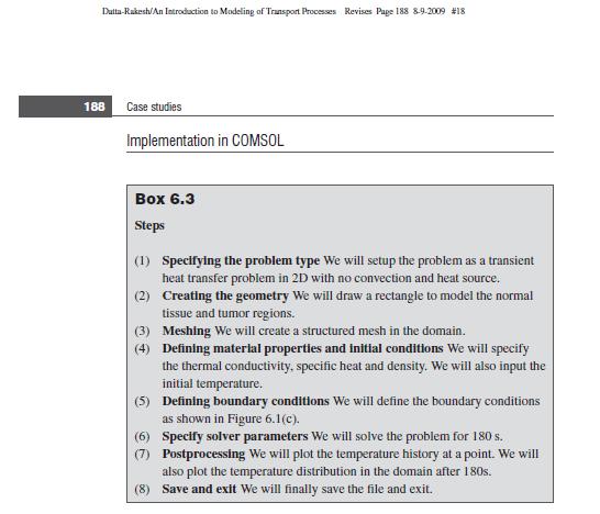
1 BEE 3500 Homework Assignment 5 Notes: For this assignment, you will use the computational software COMSOL Multiphysics 5.3, available in Academic Computing Center Engineering Library (ACCEL) at the Carpenter Hall. Rooms having access to COMSOL are the Blue Room and the Sunset Grill on the Ground Floor and the Green Room, Orange Room and Red Room on the 2nd floor. You can find when the facilities are open at Attached are the pages of a tutorial that you will complete. Instructions on what to submit is included in the following page. Although the process will not be particularly time consuming, we encourage you to get started early since we can always experience software and hardware related issues. For this week only, the TAs will be at the ACCEL facility, instead of their normal office hours. We welcome you to try out other variations of the problem in the tutorial, or any other problem that you feel like. You will find this software tool to be quite flexible and user-friendly. Please do not turn in these other results with the homework assignment.

2 Thermal ablation of hepatic tumors Go through the case study and submit the materials asked for. Each student needs to submit this individually. Color plots are not necessary. What to submit: 1) Write down the specific Governing Equation that is being solved. 2) Provide the Boundary Conditions and Initial Conditions used. 3) List clearly all the input parameter values used in consistent units. Follow the instructions given below and submit printouts for the following: 4) Create a movie of the heat conduction process. Follow these instructions to create a movie: a. After running the problem, under Model Builder >> Results, right click on Export b. Click Animation >> File. c. Under Settings >> Output >> Format, select AVI. d. Under Filename >> Browse. Input a name for the movie file and save it in desired folder. e. Select the times at which you want to save the results for the movie: under Animation Editing >> Time selection >> From list. Hold Ctrl key and select 7 different times 0, 30, 60, 90, 120, 150 and 180 by left clicking. (Note that by default all times are selected. You do not want to use that setting as the computer will need a lot of memory to make the movie file.) f. Click on Export button on top of the Settings panel or press F8. g. The address of the produced file will be shown in the Massages window (the file is saved in the same folder as the COMSOL file) h. Finally, make a contour plot of the temperature at t = 180s. Expand Isothermal Contours (ht) >> Contour. Select Study 1/Solution 1 (sol1) as Data set in Settings window and select Unit to degc. Click on Plot button next. i. Print and submit this contour plot. You do not need to submit the movie file. 5) Temperature as a function of time. a. Plot the temperature at the point (0.0075, 0.01) as a function of time. b. Save the data in text format (see instructions below) c. Change the boundary condition. The probe temperature has been set at a temperature of 90 C. Change the temperature to 70 C. d. Run the problem. e. Save the data in text format. f. Make one plot using the data obtained in steps (b) and (e) in Excel. 6) To save the data in text format: a. Plot temperature as a function of time.

3 b. Under Model Builder >> Results, expand 1D Plot Group and right click on Point Graph. c. Click on Add Plot Data to Export. d. Under Settings >> output >> Filename >> Browse. Input a name for the text file and save it in desired folder. e. Click on Export button on top of the Settings panel or press F8. f. The address of the produced file will be shown in the Massages window (the file is saved in the same folder as the COMSOL file)

4

5

6

7 SPECIFYING PROBLEM TYPE 1) Search COMSOL in the search bar and select (Classkit License) COMSOL Multiphysics 5.3 and save the file. Remember to save often to prevent losing work. 2) Select Model Wizard. 3) Select 2D under Select Space Dimension.

8 4) Under Select Physics click on the empty triangle left of Heat Transfer to expand the options >> Heat Transfer in Solids (ht). More information about Heat Transfer in Solids should appear on the right side. 5) Click on Add button at the bottom of the Select Physics box. You should see Heat Transfer in Solids (ht) in the Added physics interfaces: box. Dependent variable T (Temperature) should appear in a box on right side under Review Physics Interface. Click on green arrow Study at the bottom of the window next.

9 6) Select Time Dependent under select study. Time Dependent should appear in the Added study: box. Then click on the checked box Done at the bottom of the window.

10 CREATING THE GEOMETRY 1) In the Model Builder window, right click on Geometry 1. Select Rectangle to add new geometry. 2) In the Settings window, set the Width of rectangle as 0.06m and Height as 0.02m in Size and Shape. Then click the orange Build All Objects icon. 3) It should result in a grey rectangle in the Graphics window on the right side.

11 MESHING 1) Under Model Builder right click on Mesh 1 and select Mapped. 2) Mesh 1 option should expand and, two options - Size and Mapped 1 should appear underneath. Right click on Mapped 1 and select Distribution option. 3) Repeat step 2) to create two distributions- Distribution 1 and Distribution 2. Click on Distribution 1. Under Graphics window, click on boundary 1 and 4 (left and right boundaries of the grey rectangle. Edge of the rectangle will turn red if cursor hovers over it and turn blue after the selection.

12 4) Input Number of elements: as 20 under Distribution in Settings window. Make sure 1 and 4 appear in the Boundary Selection under Settings window. 5) Select Distribution 2. Select boundary 2 and 3 (top and bottom boundaries) in the Graphics window. Make sure 2 and 3 appear in the Boundary Selection under Settings window. Input Number of elements: as 50 under Distribution in Settings window. 6) Click on the dark blue Build All button to create a mapped mesh.

13 DEFINING MATERIAL PROPERTIES AND PARAMETERS 1) In the Model Builder expand Heat Transfer in Solids (ht) and click on Solid 1. 2) Under Heat Conduction, Solid, select User defined for Thermal conductivity (k) and input value W/m. K. Similarly, select User defined for Density (ρ) and Heat capacity at constant pressure (Cp) under Thermodynamics, Solid and input values 1060 kg/m 3 and 3600 J/kg. K respectively. 3) In the Model Builder expand Heat Transfer in Solids (ht) and click on Initial Values 1. Select User defined under Override and Contribution. Input value 310 K. 4) Right click on Heat Transfer in Solids (ht) in the Model Builder. Select Temperature to add new constant temperature boundary condition.

14 5) Under Graphics, select boundary 1 (left edge) and set boundary 1 temperature to 363 K.

15 COMPUTATION AND ANALYSIS 1) Expand Study 1 in the Model Builder and select Step 1: Time Dependent. 2) In the Setting window, change the Times under Study Settings to range(0, 1, 180). It means the simulation will run from 0 seconds to 180 seconds for time interval of 1 second. Click the icon with two blue horizontal lines for Compute next. 3) It should result in surface map at 180 seconds in the Graphics window. 4) Right click on Data Sets under Results in the Model Builder and select option Cut Point 2D.

16 5) In the Settings window, select Study 1/Solution 1 (sol1) under pulldown option for Data set. Input m for X coordinate and 0.01 m for Y coordinate. 6) Under Model Builder window, right click on Results and select 1D Plot Group. 7) Right click on 1D Plot Group 3 and select Point Graph.

17 8) In the Settings window, select Cut Point 2D 1 from pulldown options for Data set. 9) Under y-axis Data, change the Unit to degc from dropdown menu and click the plot button.

18 10) You should get temperature profile at (0.0075, 0.01) in the Graphics window. 11) Expand Temperature (ht) under Results in the Model Builder and select Surface. 12) In the Settings window, select degc from the dropdown menu for Unit under Expression. 13) Click on the folder icon with arrow for plot. You should get final surface plot in degree Celsius.

19 NOTE: You can always return to the surface plot by clicking on Temperature (ht) in the Model Builder.