CS 1674: Intro to Computer Vision. Midterm Review. Prof. Adriana Kovashka University of Pittsburgh October 10, 2016

Transcription

1 CS 1674: Intro to Computer Vision Midterm Review Prof. Adriana Kovashka University of Pittsburgh October 10, 2016

2 Reminders The midterm exam is in class on this coming Wednesday There will be no make-up exams unless you or a close relative is seriously ill!

3 Review requests I received Textures and texture representations, image responses to size and orientation of Gaussian filter banks, comparisons 4 Corner detection alg, Harris 4 Invariance vs covariance, affine intensity change, and applications to know 3 Scale-invariant detection, blob detection, Harris automatic scale selection 3 Sift and feature description 3 Keypoint matching alg, feature matching 2 Examples of how to compute and apply homography, epipolar geometry 2 Why it makes sense to use the ratio: distance to best match / distance to second best match when matching features across images Summary of equations students need to know Pyramids Convolution practical use Filters for transforming the image

4 Transformations, Homographies, Epipolar Geometry

5 2D Linear Transformations x' y' a c bx d y Only linear 2D transformations can be represented with a 2x2 matrix. Linear transformations are combinations of Scale, Rotation, Shear, and Mirror Alyosha Efros

6 2D Affine Transformations Affine transformations are combinations of Linear transformations, and Translations Maps lines to lines, parallel lines remain parallel w y x f e d c b a w y x ' ' ' Adapted from Alyosha Efros

7 Projective Transformations Projective transformations: Affine transformations, and Projective warps Parallel lines do not necessarily remain parallel w y x i h g f e d c b a w y x ' ' ' Kristen Grauman

8 How to stitch together a panorama (a.k.a. Basic Procedure mosaic)? Take a sequence of images from the same position Rotate the camera about its optical center Compute the homography (transformation) between second image and first Transform the second image to overlap with the first Blend the two together to create a mosaic (If there are more images, repeat) Modified from Steve Seitz

9 Computing the homography x x, y 1 1 1, y 1 x 2, y 2 x, y 2 2 x, x, n y n n y n To compute the homography given pairs of corresponding points in the images, we need to set up an equation where the parameters of H are the unknowns Kristen Grauman

10 Computing the homography p = Hp wx' a b c x wy' d e f y w g h i 1 Can set scale factor i=1. So, there are 8 unknowns. Set up a system of linear equations: Ah = b where vector of unknowns h = [a,b,c,d,e,f,g,h] T Need at least 8 eqs, but the more the better Solve for h. If overconstrained, solve using least-squares: min Ah b 2 Kristen Grauman

11 Computing the homography Assume we have four matched points: How do we compute homography H? h 0 ' ' ' ' ' ' y yy xy y x x yx xx y x ' ' ' ' ' p' w y w w x h h h h h h h h h H h h h h h h h h h h Derek Hoiem p =Hp Apply SVD: UDV T = A [U, S, V] = svd(a); h = V smallest (column of V corr. to smallest singular value) A

12 Transforming the second image Test point: Image 2 Image 1 canvas x, y wx wy w, w x, y To apply a given homography H Compute p = Hp (regular matrix multiply) Convert p from homogeneous to image coordinates Modified from Kristen Grauman wx' wy' w p * * * * * * H * * * x y 1 p

13 Transforming the second image Image 2 Image 1 canvas H(x,y) y y x x f(x,y) g(x,y ) Forward warping: Send each pixel f(x,y) to its corresponding location (x,y ) = H(x,y) in the right image Modified from Alyosha Efros

14 Depth from disparity We have two images taken from cameras with different intrinsic and extrinsic parameters. How do we match a point in the first image to a point in the second? image I(x,y) Disparity map D(x,y) image I (x,y ) So if we could find the corresponding points in two images, we could estimate relative depth Kristen Grauman

15 Epipolar geometry: notation X x x Derek Hoiem Baseline line connecting the two camera centers Epipoles = intersections of baseline with image planes = projections of the other camera center Epipolar Plane plane containing baseline Epipolar Lines - intersections of epipolar plane with image planes (always come in corresponding pairs) Note: All epipolar lines intersect at the epipole.

16 Epipolar constraint The epipolar constraint is useful because it reduces the correspondence problem to a 1D search along an epipolar line. Kristen Grauman, image from Andrew Zisserman

17 X X Essential matrix T RX 0 [T ] RX 0 x Let E [T x] R XEX X T EX 0 E is called the essential matrix, and it relates corresponding image points between both cameras, given the rotation and translation. Before we said: If we observe a point in one image, its position in other image is constrained to lie on line defined by above. Turns out Ex is the epipolar line through x in the first image, corresp. to x. Note: these points are in camera coordinate systems. Kristen Grauman

18 Basic stereo matching algorithm For each pixel in the first image Find corresponding epipolar scanline in the right image Search along epipolar line and pick the best match x Compute disparity x-x and set depth(x) = f*t/(x-x ) Derek Hoiem

19 Correspondence search Left Right scanline Matching cost disparity Slide a window along the right scanline and compare contents of that window with the reference window in the left image Matching cost: e.g. Euclidean distance Derek Hoiem

20 Geometry for a simple stereo system Assume parallel optical axes, known camera parameters (i.e., calibrated cameras). What is expression for Z? Similar triangles (p l, P, p r ) and (O l, P, O r ): T x l Z f x r T Z depth disparity Z f T x r x l Kristen Grauman

21 Results with window search Data Left image Right image Window-based matching Window-based matching Ground truth Ground truth Derek Hoiem

22 How can we improve? Uniqueness For any point in one image, there should be at most one matching point in the other image Ordering Corresponding points should be in the same order in both views Smoothness We expect disparity values to change slowly (for the most part) Derek Hoiem

23 Many of these constraints can be encoded in an energy function and solved using graph cuts Before Derek Hoiem Graph cuts Ground truth Y. Boykov, O. Veksler, and R. Zabih, Fast Approximate Energy Minimization via Graph Cuts, PAMI 2001 For the latest and greatest:

24 Projective structure from motion Given: m images of n fixed 3D points x ij = P i X j, i = 1,, m, j = 1,, n Problem: estimate m projection matrices P i and n 3D points X j from the mn corresponding 2D points x ij X j x 1j x 3j P 1 x 2j Svetlana Lazebnik P 2 P 3

25 Photo synth Noah Snavely, Steven M. Seitz, Richard Szeliski, "Photo tourism: Exploring photo collections in 3D," SIGGRAPH

26 3D from multiple images Building Rome in a Day: Agarwal et al. 2009

27 Recap: Epipoles Point x in left image corresponds to epipolar line l in right image Epipolar line passes through the epipole (the intersection of the cameras baseline with the image plane C C Derek Hoiem

28 Recap: Essential, Fundamental Matrices Fundamental matrix maps from a point in one image to a line in the other If x and x correspond to the same 3d point X: Essential matrix is like fundamental matrix but more constrained Adapted from Derek Hoiem

29 Recap: stereo with calibrated cameras Given image pair, R, T Detect some features Compute essential matrix E Match features using the epipolar and other constraints Triangulate for 3d structure and get depth Kristen Grauman

30 Texture representations

31 Correlation filtering Say the averaging window size is 2k+1 x 2k+1: Attribute uniform weight to each pixel Loop over all pixels in neighborhood around image pixel F[i,j] Now generalize to allow different weights depending on neighboring pixel s relative position: Non-uniform weights Kristen Grauman

32 Convolution vs. correlation Cross-correlation F u = -1, v = (i, j) Convolution H (0, 0)

33 Filters for computing gradients * = Slide credit: Derek Hoiem

34 Texture representation: example mean d/dx value mean d/dy value Win. # Win.# Win.# original image Kristen Grauman derivative filter responses, squared statistics to summarize patterns in small windows

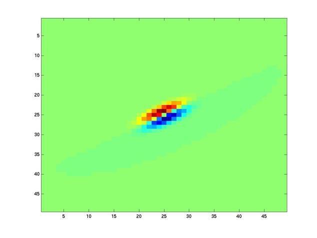
35 Filter banks orientations scales Edges Bars What filters to put in the bank? Kristen Grauman Spots Typically we want a combination of scales and orientations, different types of patterns. Matlab code available for these examples:

36 Matching with filters Goal: find in image Method 0: filter the image with eye patch g[ m, n] h[ k, l] k, l f [ m k, n l] f = image g = filter What went wrong? Derek Hoiem Input Filtered Image

37 Matching with filters Goal: find in image Method 1: filter the image with zero-mean eye g[ m, n] ( h[ k, l] mean( h)) ( k, l Likes bright pixels where filters are above average, dark pixels where filters are below average. f [ m k, n l]) True detections False detections Derek Hoiem Input Filtered Image (scaled) Thresholded Image

38 Kristen Grauman Showing magnitude of responses

39 Kristen Grauman

40 Kristen Grauman

41 Representing texture by mean abs response Filters Mean abs responses Derek Hoiem

42 Computing distances using texture Dimension 1 Dimension 2 a b #dim ) ( ), ( ) ( ) ( ), ( i a i b i b a D b a b a b a D Kristen Grauman

43 Feature detection: Harris

44 Corners as distinctive interest points We should easily recognize the keypoint by looking through a small window Shifting a window in any direction should give a large change in intensity flat region: no change in all directions A. Efros, D. Frolova, D. Simakov edge : no change along the edge direction corner : significant change in all directions

45 Harris Detector: Mathematics Window-averaged squared change of intensity induced by shifting the image data by [u,v]: Window function Shifted intensity Intensity Window function w(x,y) = or 1 in window, 0 outside Gaussian D. Frolova, D. Simakov

46 Harris Detector: Mathematics Expanding I(x,y) in a Taylor series expansion, we have, for small shifts [u,v], a quadratic approximation to the error surface between a patch and itself, shifted by [u,v]: where M is a 2 2 matrix computed from image derivatives: D. Frolova, D. Simakov

47 y y y x y x x x I I I I I I I I y x w M ), ( x I I x y I I y y I x I I I y x Notation: K. Grauman Harris Detector: Mathematics

48 What does the matrix M reveal? Since M is symmetric, we have M X X 2 T Mx i x i i The eigenvalues of M reveal the amount of intensity change in the two principal orthogonal gradient directions in the window. K. Grauman

49 Corner response function edge : 1 >> 2 2 >> 1 corner : 1 and 2 are large, 1 ~ 2 flat region: 1 and 2 are small Adapted from A. Efros, D. Frolova, D. Simakov, K. Grauman

50 Harris Detector: Algorithm Compute image gradients Ix and Iy for all pixels For each pixel Compute by looping over neighbors x, y compute (k :empirical constant, k = ) Find points with large corner response function R (R > threshold) Take the points of locally maximum R as the detected feature points (i.e., pixels where R is bigger than for all the 4 or 8 neighbors) D. Frolova, D. Simakov 55

51 K. Grauman Example of Harris application

52 Feature detection: Scale-invariance

53 Invariance vs covariance A function is invariant under a certain family of transformations if its value does not change when a transformation from this family is applied to its argument. A function is covariant when it commutes with the transformation, i.e., applying the transformation to the argument of the function has the same effect as applying the transformation to the output of the function. [ ] [For example,] the area of a 2D surface is invariant under 2D rotations, since rotating a 2D surface does not make it any smaller or bigger. But the orientation of the major axis of inertia of the surface is covariant under the same family of transformations, since rotating a 2D surface will affect the orientation of its major axis in exactly the same way. Local Invariant Feature Detectors: A Survey by Tinne Tuytelaars and Krystian Mikolajczyk, in Foundations and Trends in Computer Graphics and Vision Vol. 3, No. 3 (2007) Chapter 1, 3.2, 7

54 What happens if: Affine intensity change Only derivatives are used => invariance to intensity shift I I + b Intensity scaling: I a I I a I + b R threshold R x (image coordinate) x (image coordinate) Partially invariant to affine intensity change L. Lazebnik

55 What happens if: Image translation Derivatives and window function are shift-invariant Corner location is covariant w.r.t. translation L. Lazebnik

56 What happens if: Image rotation Second moment ellipse rotates but its shape (i.e. eigenvalues) remains the same Corner location is covariant w.r.t. rotation L. Lazebnik

57 What happens if: Scaling Corner All points will be classified as edges Corner location is not covariant to scaling! L. Lazebnik

58 Scale Invariant Detection Problem: How do we choose corresponding circles independently in each image? Do objects in the image have a characteristic scale that we can identify? D. Frolova, D. Simakov

59 Scale Invariant Detection Solution: Design a function on the region which is scale invariant (has the same shape even if the image is resized) Take a local maximum of this function f Image 1 f Image 2 scale = 1/2 Adapted from A. Torralba s 1 s 2 region size region size

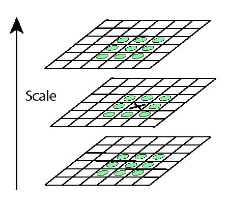
60 Automatic Scale Selection Function responses for increasing scale (scale signature) f ( I (, )) i i 1 x i i m f ( I 1 ( x, )) m K. Grauman, B. Leibe

61 Automatic Scale Selection Function responses for increasing scale (scale signature) f ( I (, )) i i 1 x i i m f ( I 1 ( x, )) m K. Grauman, B. Leibe

62 Automatic Scale Selection Function responses for increasing scale (scale signature) f I (, )) i i i i m f ( I 1 ( x, )) m K. Grauman, B. Leibe ( 1 x

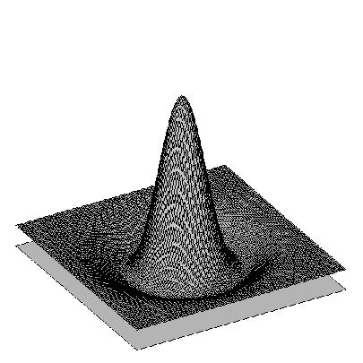
63 What Is A Useful Signature Function? Laplacian of Gaussian = blob detector K. Grauman, B. Leibe

64 Difference of Gaussian Laplacian We can approximate the Laplacian with a difference of Gaussians; more efficient to implement. 2 L Gxx x y Gyy x y (,, ) (,, ) (Laplacian) DoG G( x, y, k) G( x, y, ) (Difference of Gaussians)

65 Difference of Gaussian: Efficient computation Computation in Gaussian scale pyramid Sampling with step 4 =2 Original image K. Grauman, B. Leibe

66 Find local maxima in position-scale space of Difference-of-Gaussian 5 Position-scale space: Adapted from K. Grauman, B. Leibe Find places where X greater than all of its neighbors (in green) List of (x, y, s)

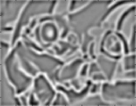
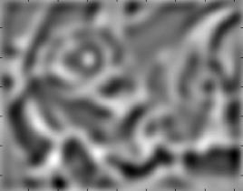
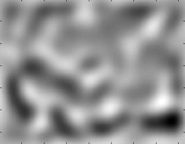
67 Laplacian pyramid example Allows detection of increasingly coarse detail

68 Results: Difference-of-Gaussian K. Grauman, B. Leibe

69 Feature description

70 Gradients m(x, y) = sqrt(1 + 0) = 1 Θ(x, y) = atan(0/1) = 0

71 Scale Invariant Feature Transform Full version Divide the 16x16 window into a 4x4 grid of cells (2x2 case shown below) Quantize the gradient orientations i.e. snap each gradient to one of 8 angles Each gradient contributes not just 1, but magnitude(gradient) to the histogram, i.e. stronger gradients contribute more 16 cells * 8 orientations = 128 dimensional descriptor for each detected feature Adapted from L. Zitnick, D. Lowe

72 Scale Invariant Feature Transform Full version Divide the 16x16 window into a 4x4 grid of cells (2x2 case shown below) Quantize the gradient orientations i.e. snap each gradient to one of 8 angles Each gradient contributes not just 1, but magnitude(gradient) to the histogram, i.e. stronger gradients contribute more 16 cells * 8 orientations = 128 dimensional descriptor for each detected feature Normalize + clip (threshold normalize to 0.2) + normalize the descriptor After normalizing, we have: such that: 0.2 Adapted from L. Zitnick, D. Lowe

73 Making descriptor rotation invariant CSE 576: Computer Vision Rotate patch according to its dominant gradient orientation This puts the patches into a canonical orientation K. Grauman Image from Matthew Brown

74 Keypoint matching

75 Matching local features? Image 1 Image 2 To generate candidate matches, find patches that have the most similar appearance (e.g., lowest feature Euclidean distance) Simplest approach: compare them all, take the closest (or closest k, or within a thresholded distance) K. Grauman

76 Robust matching???? K. Grauman Image 1 Image 2 At what Euclidean distance value do we have a good match? To add robustness to matching, can consider ratio : distance to best match / distance to second best match If low, first match looks good. If high, could be ambiguous match.

77 Ratio: example Let q be the query from the first image, d1 be the closest match in the second image, and d2 be the second closest match Let dist(q, d1) and dist(q, d2) be the distances Let r = dist(q, d1) / dist(q, d2) What is the largest that r can be? What is the lowest that r can be? If r is 1, what do we know about the two distances? What about when r is 0.1?

78 Indexing local features: Setup When we see close points in feature space, we have similar descriptors, which indicates similar local content. Descriptor s feature space Query image K. Grauman Database images

79 Image matching

80 times appearing times appearing times appearing Describing images w/ visual words Summarize entire image based on its distribution (histogram) of word occurrences. Analogous to bag of words representation commonly used for documents. Feature patches: K. Grauman Visual words

81 Bag of visual words: Two uses 1. Represent the image 2. Using that representation, look for similar images 3. Can also use BOW to compute an inverted index, to simplify application #2

82 Visual words: main idea Extract some local features from a number of images e.g., SIFT descriptor space: each point is 128-dimensional D. Nister, CVPR 2006

83 D. Nister, CVPR 2006 Visual words: main idea

84 D. Nister, CVPR 2006 Quantize the space by grouping (clustering) the features. Note: For now, we ll treat clustering as a black box.

85 Inverted file index and bags of words similarity w (offline) Extract features in database images, cluster them to find words, make index 2. Extract words in query (extract features and map each to closest cluster center) 3. Use inverted file index to find frames relevant to query 4. For each relevant frame, rank them by comparing word counts (BOW) of query and frame Adapted from K. Grauman

86 precision Scoring retrieval quality Query Database size: 10 images Relevant (total): 5 images (e.g. images of Golden Gate) Results (ordered): precision = # returned relevant / # returned recall = # returned relevant / # total relevant Ondrej Chum recall