µ = Pa s m 3 The Reynolds number based on hydraulic diameter, D h = 2W h/(w + h) = 3.2 mm for the main inlet duct is = 359

Transcription

1 Laminar Mixer Tutorial for STAR-CCM+ ME 448/548 March 30, 2014 Gerald Recktenwald 1 Overview Imagine that you are part of a team developing a medical diagnostic device. The device has a millimeter scale flow channel designed to allow a sample fluid to be mixed with a carrier fluid. Figure 1 is a top-view schematic of the base case design for the flow channel. Figure 2 is a three-dimensional model created in Solidworks. The dimensions of the channel are L = 50, L i = 6, L s = 5, W = 8, w s = 2, h = 2 where h is the depth of the channel (into the page) and all lengths are in mm. In the test apparatus, water is used for both the carrier fluid and the sample fluid. The sample fluid is marked with red food coloring to provide a visual indication of how well the sample fluid mixes with the carrier fluid. The carrier stream has a velocity of V in = 0.1 m/s and the sample stream has an inlet velocity of V s = 0.05 m/s. The properties of water used by STAR-CCM+ are ρ = kg m 3 µ = Pa s The Reynolds number based on hydraulic diameter, D h = 2W h/(w + h) = 3.2 mm for the main inlet duct is Re Dh = ρv ind h µ = 359 Measurements show that despite the intention of the designers, the channel does a poor job of mixing the sample fluid with the carrier fluid. Your job is to propose design changes that will improve the mixing. Your design changes cannot alter the overall dimensions L, W, w s, L s or h. You cannot change the sample L i w s L s water W L Figure 1: Device for testing flow mixing strategies.

2 2 IMPORT THE MODEL GEOMETRY 2 Figure 2: Solidworks model of the flow channel. fluid velocities V in and V s. You can alter the geometry of the channel, for example, by adding obstructions or objects to increase mixing. Any modifications should be geometrically simple so that the new design is easy to manufacture. The three-dimensional geometry of the channel was created in Solidworks model and saved as a Parasolid XT CAD file 1 that is imported into STAR-CCM+ as a surface mesh. 2 Import the Model Geometry The model geometry is defined in a Parasolid file stored as microchanel_mixer.x_t. Download that file from and store it in a convenient place. 2.1 Import the Parasolid Surface Mesh The Parasolid model defines a geometry in a form that STAR-CCM+ can understand, but not work with directly. 1 Parasolid is a 3D geometric modeling engine owned by Siemens. See automation.siemens.com/en_us/products/open/parasolid/index.shtml.

3 2 IMPORT THE MODEL GEOMETRY 3 1. Launch STAR-CCM+ and open a new simulation. 2. Import the surface mesh: a. File Import Import Surface Mesh. b. Select the microchanel_mixer.x_t file from your computer s drive. c. In the Import Surface Options dialog box, make sure the Create New Part option is selected. d. Click OK. 2.2 Split the Single Surface into Patches The surface mesh in the Parasolid model is a network of triangles that define the geometric features of the surface that encloses the domain volume. This single surface must be separated so that boundary conditions can be applied to distinct areas on the boundary of the domain. The first step in that process is to split the one bounding surface into patches, where each patch is a area that defines a smaller piece of the surface geometry. After the dividing the surface into patches, we rename those patches, and in some cases regroup the patches to form boundaries. When the patches are renamed and regrouped, we are ready to assign those patches to the boundaries of the region in Section Select the new part in the Geometry tree 2. Expand the Surfaces node 3. Right-click on Faces and select Split by Patch.... Notice these features of the user interface as evident in Figure 3: The Geometry Scene now has different color surface patches. Each surface patch corresponds to a number listed in the edit panel in the upper left. Surface patches are selected by either clicking on their number or clicking on the patch in the Geometry Scene.

4 2 IMPORT THE MODEL GEOMETRY 4 Figure 3: Appearance of the Geometry Scene and the edit panel used to select and name patches. 4. Orient the model in the Geometry Scene so that you can select (click on) the outlet face as shown in Figure In the edit panel in the upper left, type outlet into the Part Surface Name box and click Create. This will rename the surface patch and remove it from the display in the Geometry Scene. It is possible to select and name multiple patches at a time with this procedure, which has the effect of merging those patches. For the current model, we will only work with one patch at a time. 6. Repeat the two preceding steps for the two inlets. Choose inlet_main and inlet_sample for the names of the main inlet surface and sample inlet surface, respectively. 7. Click Close to stop selection of the patches. Notice that under the Surfaces node (a sub-node of the Parts) that there are separate surfaces: the three newly created and named surfaces (inlet_main, inlet_sample and outlet, and one remaining surface called Faces. 8. Select the Faces surface, right-click to select Rename... and change the name to duct_wall. 2.3 Save the Model Select Save from the file menu to save the model in a.sim file on the hard drive of your computer. It s a good idea at this point to create a directory for the

5 3 CREATE FLUID REGION AND BOUNDARIES 5 simulation results as well as a meaningful file name. As you build the model and run different cases, you will accumulate alternate.sim files for the same physical problem. You will also generate external graphics files to be incorporated into reports. Therefore, creating a directory to group the files related to a single simulation will help you stay organized later. Click the Save icon. 3 Create Fluid Region and Boundaries The volume occupied by the part must be assigned to a Region. This can be accomplished (at least) two ways. Choose only one of the following 1. Assign the Part to a Region. or 2. Create a new Region, and then select the parts that belong to it. The procedures are equivalent. We will demonstrate both. When you build your model, follow the steps in either Section 3.1 or Section 3.2, but not both. 3.1 Assign Parts to Regions 1. Right click on the part node (first level under Parts) and select Assign Parts to Regions...

6 3 CREATE FLUID REGION AND BOUNDARIES 6 2. In the Assign Parts to Regions dialog box, make sure the Part is selected 3. Click the Create Regions button 4. Click Close

7 3 CREATE FLUID REGION AND BOUNDARIES Create a Region and Assign Parts to It The following steps are an alternative to the steps in Section Select Regions, right-click New 2. Right-click on the newly-created region, and select Rename Enter fluid as the fluid name. Click OK. Assign the Part to the fluid Region. 1. Click on the fluid node to select it. 2. In the Properties pane (lower left corner), click the [... ] icon to initiate selection of the parts for the Region. 3. In the dialog box, select the Part corresponding to the fluid by clicking the blue dot to the left of the part name. 4. Click OK. 3.3 Create Boundaries of the Region Now that the fluid region is created (using the procedure in Section 3.1 or Section 3.2), we must separate the bounding surface of the region into four separate surfaces, one for each type of boundary condition. 1. Inlet for the main stream: velocity inlet with V in = 0.1 m/s and zero concentration of the passive scalar. 2. Inlet for the sample stream: velocity inlet with V s = 0.05 m/s and concentration of the passive scalar set to 0.5. The concentration of the passive scalar is arbitrary for this problem. 3. Single outlet: pressure boundary condition. 4. Solid walls. The default condition for a region boundary is a solid wall. The procedure is to assign the two inlets and the outlet to new boundary surfaces. The left-over surface, which is composed of several rectangular patches, is the wall. At this stage we can only assign the type of boundary condition, not the values of the fluid properties on the boundary. Values of fluid properties can be assigned only after the fluid continuum is defined. Therefore, if we skipped

8 3 CREATE FLUID REGION AND BOUNDARIES 8 ahead to complete the steps in Section 4, then it would be possible to assign values to the boundary conditions at the same time that the boundary conditions types are specified. The values of properties at the boundary are assigned in Section One outlet boundary Separate the outlet surface and assign its boundary type. 1. Expand the Boundaries node under the fluid Region. 2. Right-click on Boundaries and select New. 3. Right-click on the newly-created Boundary 1 node and select Rename Enter outlet in the New Name field. Click OK. 5. Select the newly created outlet boundary surface. 6. In the Properties pane (lower left corner), Click the [... ] icon to initiate selection of part surfaces for the outlet boundary. 7. In the dialog box, expand the Part node and select the sub-part corresponding to the outlet by clicking the blue dot to the left of the part name. 8. In the Properties pane (lower left corner), Click in the box to the right of Type. Select Pressure Outlet from the pop-up menu of options Two inlet boundaries Separate the inlet_main and inlet_sample surfaces and assign the boundary type to those surfaces. The procedure is the same as that used for the outlet boundary, with the exception, of course, that a different boundary names and boundary types and applied to different part surfaces. 1. Right-click on Boundaries and select New. 2. Right-click on the newly-created Boundary (currently Boundary 1 ) and select Rename Enter inlet_main in the New Name field. Click OK. 4. Select the newly created boundary surface (inlet_main) 5. In the Properties pane (lower left corner), Click the [... ] icon to initiate selection of part surfaces for the inlet_main boundary. 6. In the dialog box, expand the Part node and select the sub-part corresponding to the main inlet by clicking the blue dot to the left of the part name. 7. In the Properties pane (lower left corner), Click in the box to the right of Type. Select Velocity inlet from the pop-up menu of options. We will specify the value of this velocity later. Repeat the preceding steps, substituting inlet_sample for inlet_main while selecting the sample inlet surface instead of the main inlet.

9 4 CREATE THE FLUID CONTINUA Save the Model Click the Save icon. 4 Create the Fluid Continua This problem introduces the passive scalar, which will be used as a marker to indicate the degree of mixing. A passive scalar is a quantity of interest that is transported by convection and diffusion. It is passive in the sense that its presence does not affect the motion of the fluid. We will call the passive scalar red dye to reinforce the idea that the passive scalar could be red food coloring that is uniformly mixed into the sample stream. 4.1 Turn on the features of the Physics Continuum Except for the turning on the passive scalar feature, all other fluid continuum features are the typical ones for steady, laminar flow. 1. Right-click Continua, select New Physics Continua. 2. Make the following choices for the phyisics models Three-dimensional Steady Liquid Segregated Flow Constant Density Laminar Passive Scalar 3. Click Close 4.2 Create the red dye passive scalar Checking the Passive Scalar box in the Physics Continuum model causes the Passive Scalar feature to be enabled. We must also define that Passive Scalar, i.e., we must identify the red dye as a passive scalar 1. Expand the Passive Scalar node in the Physics 1 Models tree. 2. Right-click on Passive Scalars New 3. Right-click on the newly created Passive Scalar node and select Rename Enter red dye as the new name of the passive scalar 4.3 Save the Model Click the Save icon.

10 5 SPECIFY VALUES OF BOUNDARY PROPERTIES 10 5 Specify values of boundary properties The type of boundaries were specified when the surfaces of the Region were created. After Physics Continuum is created, the values of the fluid properties on the surface can be specified. 1. On the inlet_main surface Velocity: 0.1 m/s. Passive scalar: [0.0] (the default) 2. On the inlet_sample surface Velocity: 0.05 m/s. Passive scalar: [0.50] (arbitrary, but non-zero) The default values on the outlet and wall boundaries are correct. 6 Create the Mesh 1. Right-click Continua, select New Mesh Continua. 2. Make the following choices for the mesh models Surface Remesher Polyhedral Mesher Prism Layer Mesher 3. Click Close 6.1 Select dimensions controlling the mesh size The smallest dimensions in the physical problem are h = 2 mm and w s = 2 mm. Keep these values in mind when specifying the mesh base size and the thickness of the prism layer, which should be smaller than the smallest macroscopic feature in the domain Set the base size 1. Expand the Reference Values node of the Mesh tree 2. Select Base Size node 3. Set the value of base size to m or 0.5 mm.

11 6 CREATE THE MESH 11 Import surface mesh Launch surface repair Clear generated meshes Generate surface mesh Generate volume mesh Initialize meshing Figure 4: Icons in the menubar for meshing tasks Adjust the prism layer properties 1. Click on the Number of Prism Layers node in the Mesh tree. 2. In the Properties pane, change Number of Prism Layers to Click on the Prism Layer Thickness node 4. In the Properties pane, change Size type to Absolute. 5. Expand the Prism Layer Thickness node of the Mesh tree. 6. In the Properties pane, change Value (of Prism Layer Thickness) to mm. 6.2 Generate and inspect the mesh Figure 4 shows the six buttons in menu bar that initiate meshing operations. For basic fluid models, the Clear generated meshes and Generate volume mesh buttons are most frequently used. 1. Click on the Generate volume mesh icon 2. Open a new Mesh Scene by Right-clicking on Scenes New Scene Mesh The Mesh Scene pane will show one of four representations of the mesh: Geometry, Initial Surface, Remeshed Surface, Volume. Figure 5 shows three of those representations. The Geometry and Initial Surface representations show the triangles (sometimes very long and skinny triangles) used by the CAD tool to define the surface of the domain. The Remeshed Surface is also a geometrydefining mesh created by the Surface Remesher. The Volume Mesh depends on the kind of volume mesher selected for the Mesh Continuum. Figure 5 shows the volume mesh at the outlet when the Prism Layer and Polyhedral volume mesh options are selected. There are many ways to control the size of the volume mesh elements. The primary control is via the base size parameter. Figure 6 shows the mesh on the outlet surface for two choices of base size: 0.5 mm and 0.2 mm. 6.3 Save the Model Click the Save icon.

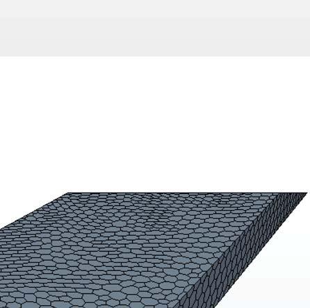
12 6 CREATE THE MESH 12 Geometry: Parasolid mesh Geometry: zoom near outlet Volume mesh Remeshed surface Figure 5: Three representations of the mesh in the Mesh Scene: Remeshed Surface, Volume Mesh. Geometry, Figure 6: Mesh on the outlet surface for base size of 0.5 mm (top) and 0.2 mm (bottom).

13 7 RUN THE MODEL 13 Step Run Initialize Stop Figure 7: Icons in the menubar for running, stepping and stopping a simulation. 7 Run the model Figure 7 shows the four buttons in menu bar that are used to run, step and stop a solution. The start button is frequently used to begin the simulation. Clicking the run button automatically initializes the solution if it hasn t already been initialized. Clicking the run button will continue a simulation that has already taken some iterations. If you click on the stop button, the solver completes the current iteration before stopping. Therefore, clicking stop will not risk damage to a successful simulation. The step button causes the solver to complete one more iteration. 7.1 Limit the number of time steps 1. Expand Stopping Criteria node 2. Click Maximum Steps and set to Add stopping criterion for continuity residuals 1. Right-click on the Stopping Criteria node 2. Select Create New Criterion Create from Monitor Continuity 3. Click on the Minimum Limit sub-node 4. Notice that the Minimum Value in the Properties Pane is 1.0E-4. Leave this value for now. 7.3 Start the solver 1. Click the Run icon 2. Watch the residual plot. If the residual plot does not automatically open in the Scene pane, expand the Plots node in the simulation tree, then right-click on the Residuals node and select Open. The residual plot to the right shows that the model converges in about 100 iterations.

14 8 VISUALIZE THE RESULTS 14 8 Visualize the Results 8.1 Red dye concentration Red dye from the sample inlet is convected downstream after it enters the main channel. The dye also slowly diffuses into the water from the main channel flow Dye concentration a horizontal plane in middle of the duct Create a plane for visualizing the x z distribution of red dye in the channel. 1. Bring the Geometry Scene tab to the foreground 2. Right-click on Derived Part New Section Plane This opens an edit panel in the upper left corner. 3. Click on Select... in the Input Parts area at the top of the edit panel. 4. Select the channel fluid region (or whatever you named the Region) 5. Enter the values to the right into the Plane Parameters table. Any x and z values will work in the origin column. 6. Click Create origin normal x 0 mm 0 mm y 1 mm 1 mm z 0 mm 0 mm 7. Click Close 8. In the list of Derived Parts, right-click on the newly created plane section and select Rename.... Change the name to y-normal midplane or some other meaningful name. 9. Click OK. Create a scalar viewer to display the concentration on the horizontal midplane. 1. Right-click on Scenes New Scene Scalar 2. Expand the newly created Scalar Scene 1 node. (At this point you could rename the scene to make it easier to identify at later stages in model development and visualization.) 3. Click on the Parts node under the Scalar 1 node of the newly created Scalar Scene. 4. In the Properties pane, click on the [... ] icon to the right of the Parts item. 5. Select the y-normal midplane from the list of Derived Parts (Be sure to click on the blue square, not the name of the part.) 6. Click OK to close the parts selection dialog box 7. Click on the Scalar Field node under the Parts sub-node 8. In the Properties pane, click on the <Select Function> field in the Function row. Select Passive Scalar red dye

15 8 VISUALIZE THE RESULTS Click on the Scalar 1 node 10. In the Properties pane, click on the Filled field in the Contour Style row. Select Smooth Filled from the pop-up menu. 11. Click on the Outline 1 node under the Displayers node of the Scalar Scene. 12. In the Properties pane, check the Feature lines box Figure 8 shows two view of the image created by the preceding steps. The views are created by the rotating the model in the Scalar Scene viewer. Standard views and user-define views can be defined and recalled by clicking the Save-Restore-Select views button and choosing views +Y Up +X. Figure 8: Two views of the concentration of red dye on the mid plane for the coarse mesh solution.

16 8 VISUALIZE THE RESULTS Concentration profile at the exit mid-plane Creation of a concentration profile at the exit is a two-step process. 1. Create a line probe to extract data from the field values on the mesh 2. Create an X-Y plot to display the profile data Create a line probe 1. Open the Geometry Scene tab 2. Right-click on Derived Parts New Part Probe Line.... This opens an edit panel in the upper left corner. 3. Click on Select... in the Input Parts area at the top of the edit panel. 4. Select the outlet boundary in the fluid region 5. Enter the following values for the coordinates of Point 1 and Point 2 Point 1 Point 2 x 0 mm 8 mm y 1 mm 1 mm z 45 mm 45 mm Inspect the image in the Geometry Scene to verify that the line probe is correctly located.

17 8 VISUALIZE THE RESULTS Click Create 7. Click Close. 8. In the list of Derived Parts, right-click on the newly created line probe and select Rename.... Change the name to exit profile probe. Click OK Plot the concentration data on the line probe Now that the probe line has been created, we can construct the plot 1. Right-click on the Plots node. 2. Select New Plot X-Y 3. Right-click on the new XY Plot 1 node and select Rename.... Give the plot a new name, like exit profile 4. In the Properties pane, Click on the [... ] icon for the Parts property 5. Select the outlet boundary as the Part to be used for the plot data. 6. Expand the X Type node and click on the Position sub-node 7. In the Properties panel, note that the Direction value is [1.0, 0.0, 0.0] which corresponds to having the independent (X Type) value equal to the x axis. This is correct for the profile we want to create. 8. Expand the Y Types node 9. Expand the Y Type 1 sub-node 10. Click on the Scalar sub-node 11. In the Properties pane, select Passive Scalar red dye. 12. The appearance of the plot can be improved by adjusting the symbol type, x axis range, and x-axis label spacing. First, change the axis range. a. Expand the Axis node. Expand the X Axis sub-node. Expand the Title sub-node. b. Click on the Labels sub-node. c. In the Properties pane, change the Maximum property to 0.008, and change the Label Spacing to Next change the symbol type a. Expand the Y Types node. Expand the Y Type 1 sub-node. Expand the exit profile probe sub-node. (exit profile probe is the name of the line probe derived part. b. Click on Symbol Style. c. In the Properties pane, change the Size to 8. Change the Shape to Dot. Change the Color to Black. The result of these operations is the plot in Figure 9.

18 8 VISUALIZE THE RESULTS 18 Figure 9: Profile of red dye concentration across the x direction at the duct exit Export the profile data to a CSV file To post-process the data in Matlab or Excel, export the profile data to a CSV file. 1. Right click on exit profile the name of the X-Y plot under the Plots node. 2. Select Tabulate Click Export... in the Tabular Data dialog box 4. Navigate to a good place in your file system and enter a name like dye_exit_profile.csv in the File name: field and click Save. 8.3 Save the Model Click the Save icon.

19 8 VISUALIZE THE RESULTS Streamlines Create Streamline Derived Parts Streamlines are geometric features derived from the velocity field. The Derived Part interface is used to specify the seed point (or points) of the streamlines. We will create two separate line seeds. After the seeds are defined, and after the velocity field has been obtained, the streamlines are visualized in a Scene. 1. Open the Geometry Scene tab. 2. Right-click on Derived Parts New Part Streamline.... This opens an edit panel in the upper left corner. It also opens up a pop-up window that a 3. Make sure that the Input Parts selection is for the fluid domain, e.g., it is not empty or referring to a boundary 4. Make sure Vector Field is set to Velocity 5. In the Seed Mode pop-up menu, select Line Seed. 6. Enter the following values for the coordinates of Point 1 and Point 2. Point 1 Point 2 x 7.5 mm 7.5 mm y 0 mm 2 mm z 0 mm 0 mm If the model includes a velocity field (i.e., if the flow solver has been run and there is a velocity field in the current model) the streamlines should be visible in the Geometry Scene. 7. Set the resolution (number of points) to Click Apply. You should now see faint streamlines in the Geometry Scene. 9. Enter the following values for the coordinates of Point 1 and Point 2. Point 1 Point 2 x mm mm y 0 mm 2 mm z 7.75 mm 7.75 mm The x coordinates are just shy of the 13 mm that defines the far edge of the domain. Due to round-off, the streamline seed may fall outside of the domain if x = 13 mm is used to define the seed line. This may or may not be an issue in your model. Using x = mm guarantees that the see line is inside the domain. 10. Click Apply. A new set of streamlines should be visible in the Geometry Scene. 11. Click Close.

20 8 VISUALIZE THE RESULTS 20 Figure 10: Stream tubes emanating from the two inlets for the coarse mesh solution with base size = 0.5 mm Display the Streamlines Once streamlines are created with the preceding steps, those streamlines can be added to any Scene. 1. In any Scene, right-click on the Displayers node and select New Displayers Streamline. 2. Expand the Streamlines 1 node. 3. In the Properties pane, change Mode to Tube. This changes the streamlines to stream tubes, but the scale of the tubes is so large that they obliterate the other features of the Scene. Change the Width parameter in the Properties pane to 1e-4 to give the stream tubes an appropriate scale. 4. Click on the Scalar Field sub-node of the Streamline 1 node. In the Properties pane, click on <Select Function> adjacent to the Function property, and select Velocity Magnitude. Repeat the preceding steps for the second streamline part. When scalars are displayed on more than one set of streamlines, it is very important that the scalars use the same scale. Figure 10 shows two sets of stream tubes (created with the preceding steps) and a single color scale to indicate the velocity magnitude. 1. Select Scalar Field sub-node of the Streamline 1 node a. In the Properties pane, set the min value to 0. b. Set the max value to a value somewhat larger than the default value. In this example a maximum value of 0.16 is sufficient. 2. Select Scalar Field sub-node of the Streamline 2 node a. In the Properties pane, set the min value to 0. b. Set the max value to the same value as the maximum for the velocity scale used in the other streamline object.

21 9 QUANTITATIVE REPORTS 21 c. Click on the Color Bar sub-node for that Scalar Field and uncheck the Visible box. The preceding steps should yield a stream tube plot similar to that in Figure Quantitative Reports 9.1 Element Counts 1. Right-click Reports New Report Element Count 2. Click on the just-created Element Count 1 sub-node 3. In the Properties pane, click on the [... ] icon in the Parts row. 4. Select all of the nodes under the fluid region (under the Regions node). Make sure you click the blue squares, not the names of the region or boundary. 5. Right-click on Element Count 1 Run Report. The results of the report are printed to the Output pane. Element Count Part Element Count channel e+04 cells channel_side_mix.inlet_main e+02 faces channel_side_mix.inlet_sample e+02 faces channel_side_mix.outlet e+02 faces channel_side_mix.walls e+03 faces Total: e+04 element

22 9 QUANTITATIVE REPORTS Average Pressures on inlets and outlet 1. Right-click Reports New Report Surface Average 2. Click on the just-created Surface Average 1 sub-node 3. In the Properties pane, click on the [... ] icon in the Parts row. 4. Select two inlet and one outlet surfaces under the fluid region (under the Regions node). Make sure you click the blue squares, not the names of the region or boundary. 5. In the Properties pane, click on the <Select Function> field in the Scalar Function Row row. Select Pressure 6. Right-click on Surface Average 1 Run Report. The results of the report are printed to the Output pane. Surface Average of Pressure on Volume Mesh Part Value (Pa) channel: channel_side_mix.inlet_main e+01 channel: channel_side_mix.inlet_sample e+01 channel: channel_side_mix.outlet e Total: e Save the Model Click the Save icon.