Introduction to Comsol Multiphysics

Transcription

1 Introduction to Comsol Multiphysics VERSION 4.3

2 Introduction to COMSOL Multiphysics COMSOL Protected by U.S. Patents 7,519,518; 7,596,474; and 7,623,991. Patents pending. This Documentation and the Programs described herein are furnished under the COMSOL Software License Agreement ( and may be used or copied only under the terms of the license agreement. COMSOL, COMSOL Desktop, COMSOL Multiphysics, Capture the Concept, and LiveLink are registered trademarks or trademarks of COMSOL AB. AutoCAD and Inventor are registered trademarks of Autodesk, Inc., in the USA and other countries. LiveLink for AutoCAD and LiveLink for Inventor are not affiliated with, endorsed by, sponsored by, or supported by Autodesk, Inc., and/or its affiliates and/or subsidiaries. MATLAB is a registered trademark of The Mathworks, Inc. Pro/ENGINEER is a registered trademark of Parametric Technology Corporation or its subsidiaries in the U.S. and in other countries. SolidWorks is a registered trademark of Dassault Systèmes SolidWorks Corp. SpaceClaim is a registered trademark of Space- Claim Corporation. Other product or brand names are trademarks or registered trademarks of their respective holders. Version: May 2012 COMSOL 4.3 Contact Information Visit for a searchable list of all COMSOL offices and local representatives. From this web page, search the contacts and find a local sales representative, go to other COMSOL websites, request information and pricing, submit technical support queries, subscribe to the monthly enews newsletter, and much more. If you need to contact Technical Support, an online request form is located at Other useful links include: Technical Support Software updates: Online community: Events, conferences, and training: Tutorials: Knowledge Base: Part No. CM010004

3 Contents Introduction The COMSOL Desktop Thorough Example: The Busbar Parameters, Functions, Variables, and Model Couplings Material Properties and Libraries Mesh Sequences Adding Physics to a Model Parameter Sweeps Parallel Computing Geometry Sequences Easy Example: The Wrench COMSOL Multiphysics Additional Concepts Working with 3D Geometry in the Graphics Window Keyboard Shortcuts Finding More Information Supported External File Formats

4 4

5 Introduction Computer simulation has become an essential part of science and engineering. Digital analysis of components, in particular, is important when developing new products or optimizing designs. Today a broad spectrum of options for simulation is available; researchers use everything from basic programming languages to various high-level packages implementing advanced methods. Though each of these techniques has its own unique attributes, they all share a common concern: Can you rely on the results? When considering what makes software reliable, it s helpful to remember the goal: you want a model that accurately depicts what happens in the real world. A computer simulation environment is simply a translation of real-world physical laws into their virtual form. How much simplification takes place in the translation process helps to determine the accuracy of the resulting model. It would be ideal, then, to have a simulation environment that included the possibility to add any physical effect to your model. That is what COMSOL is all about. It s a flexible platform that allows even novice users to model all relevant physical aspects of their designs. Advanced users can go deeper and use their knowledge to develop customized solutions, applicable to their unique circumstances. With this kind of all-inclusive modeling environment, COMSOL gives you the confidence to build the model you want with real-world precision. Certain characteristics of COMSOL become apparent with use. Compatibility stands out among these. COMSOL requires that every type of simulation included in the package has the ability to be combined with any other. This strict requirement actually mirrors what happens in the real world. For instance in nature, electricity is always accompanied by some thermal effect; the two are fully compatible. Enforcing compatibility guarantees consistent multiphysics models, and the knowledge that, even as the COMSOL family of products expands, you never have to worry about creating a disconnected model again. Another noticeable trait of the COMSOL platform is adaptability. As your modeling needs change, so does the software. If you find yourself in need of including another physical effect, you can just add it. If one of the inputs to your model requires a formula, you can just enter it. Using tools like parameterized geometry, interactive meshing, and custom solver sequences, you can quickly adapt to the ebbs and flows of your requirements. Introduction 5

6 COMSOL Multiphysics also has several problem-solving benefits. When starting a new project, using COMSOL helps you understand your problem. You are able to test out various geometrical and physical characteristics of your model, so you can really hone in on the important design challenges. The flexible nature of the COMSOL environment facilitates further analysis by making what-if cases easy to set up and run. You can take your simulation to the production level by optimizing any aspect of your model. Parameter sweeps and target functions can be executed right in the user interface. From start to finish, COMSOL is a complete problem-solving tool. As you become a more experienced user of COMSOL, your confidence in computer simulation will grow. You will become a more efficient modeler, and the results will show it. The remainder of this introduction is dedicated to give you a strong start toward this goal. After a general introduction to the user interface, several tutorials will take you step by step through sample models that highlight important features. The informative charts give you an idea of COMSOL s capability by associated files, functions, and built-in options. By the end you will be well on your way to reaping all the benefits that COMSOL has to offer. 6 Introduction

7 The COMSOL Desktop The user interface streamlines the modeling workflow with the Model Builder. Containing a Model Tree, the Model Builder outlines the structure of your model. Look at this example of the Model Builder. Every step of the modeling process, from defining global variables to the final report of results, is displayed in the Model Tree. When you right-click any node in the tree, a context menu shows the available features. In addition, many nodes can be easily moved up and down in the model tree by dragging and dropping the nodes. You can also right-click to copy, delete, disable, or enable nodes. The COMSOL Desktop 7

8 If you choose an action that requires specification, the matching settings window displays next to the Model Builder: A selected node and its settings window. Click any associated node to return to a specific settings window. As you create the model, each step is shown in the Model Builder. If, for example, your model required a certain sequence of steps to get the right geometry, these are all listed in the order you set. This series of steps can be edited and rerun without having to repeat the entire simulation. Complicated solver sequences you may need for different studies also benefit greatly from this feature. As you work with the COMSOL Desktop and the Model Builder, you will grow to appreciate the organized and streamlined approach. But any description of a user interface is inadequate until you try it for yourself. So in the next few sections, you are invited to work through some examples to familiarize yourself with the software. 8 The COMSOL Desktop

9 Thorough Example: The Busbar Electrical Heating in a Busbar In order to get acquainted with COMSOL Multiphysics, it is best to work through a basic example step by step. These instructions describe the essential components of the model building procedure, highlighting several features and demonstrating the common simulation tasks. At the end, you will have built a truly multiphysics model. The model that you are about to create analyzes a busbar designed to conduct direct current to an electric device (see below). The current conducted in the busbar, from bolt 1 to bolts 2a and 2b, produces heat due to the resistive losses, a phenomenon referred to as Joule heating. The busbar is made of copper while the bolts are made of a titanium alloy. The choice of materials is important because titanium has a lower electrical conductivity than copper and will be subjected to a higher current density. Titanium Bolt 2a Titanium Bolt 2b Titanium Bolt 1 The goal of your simulation is to precisely calculate how much the busbar heats up. Once you have captured the basic multiphysics phenomena, you will have the chance to investigate thermal expansion yielding structural stresses and strains in the busbar and the effects of cooling by an air stream. The Joule heating effect is described by conservation laws for electric current and energy. Once solved for, the two conservation laws give the temperature and electric field, respectively. All surfaces, except the bolt contact surfaces, are cooled by natural convection in the air surrounding the busbar. You can assume that the bolt cross-section boundaries do not contribute to cooling or heating of the device. The electric potential at the upper-right vertical bolt surface is 20 mv, and that the potential at the two horizontal surfaces of the lower bolts is 0 V. Thorough Example: The Busbar 9

10 Busbar Model Overview More in depth and advanced topics included with this tutorial are used to show you some of the many options available in COMSOL. The following topics are covered: Parameters, Functions, Variables, and Model Couplings on page 36, where you learn how to define functions and model couplings. Material Properties and Libraries on page 41 shows you how to customize a material and add it to your own material library. Mesh Sequences on page 43 gives you the opportunity to add and define two different mesh nodes and compare two meshes generated and displayed in the Graphics window. Adding Physics to a Model on page 45 explores the multiphysics capabilities by adding a Solid Mechanics interface and a Laminar Flow interface to the busbar model. Parameter Sweeps on page 64 gives you some practice of how to make minor changes to the busbar design and quickly view the differences in the Graphics window. Use this analysis to make design changes to a model. In the section Parallel Computing on page 71, you experiment with adding a Cluster Computing node. The last section, Geometry Sequences on page 73, contains the step-by-step instructions to build the busbar geometry yourself instead of importing or opening it from a file. MODEL WIZARD 1 Open the Model Wizard. To open the Model Wizard, double-click the COMSOL icon on the desktop. Or when COMSOL is already open: - Click the New button on the main toolbar - Select File>New from the main menu - Right-click the root node and select Add Model 10 Thorough Example: The Busbar

11 2 When the Model Wizard opens, select a space dimension; the default is 3D. Click the Next button. 3 In the Add Physics window, click the Heat Transfer>Electromagnetic Heating folder, then right-click Joule Heating and choose Add Selected. Click the Next button. You can also double-click or click the Add Selected button to add physics. Another way to open the Add Physics window is to right-click the Model node and select Add Physics. 4 In the Select Study Type window, click to select the Stationary study type. Click the Finish button. Preset Studies are studies that have solver and equation settings adapted to the selected physics, in this example, Joule heating. Any selection from the Custom Studies branch needs manual fine-tuning. Thorough Example: The Busbar 11

12 GLOBAL DEFINITIONS If you want to draw the geometry yourself, the Global Definitions branch is where you define the parameters. First complete the section Geometry Sequences on page 73 and then return to this section and use this busbar.mph file. If you would prefer to load the geometry from a file, you can just browse through this section and then skip to Geometry on page 13. 2xrad_1 The Global Definitions node in the Model Builder stores Parameters, Variables, and Functions with a global scope. You can use these operations in several models. In this case, there is only one Model 1 node where the parameters are used. Since you will run a geometric parameter study later in this example, define the geometry using parameters from the start. In this step, enter parameters for the length for the lower part of the busbar, L, the radius of the titanium bolts, rad_1, the thickness of the busbar, tbb, and the width of the device, wbb. You will also add the parameters that control the mesh, mh, a heat transfer coefficient for cooling by natural convection, htc, and a value for the voltage across the busbar, Vtot. 1 Under Global Definitions click the Parameters node. In the Parameters table, click the first row under Name and enter L. 2 Click the first row under Expression and enter the value of L, 9[cm]. You can enter any unit inside the square brackets. wbb tbb L 12 Thorough Example: The Busbar

13 3 Continue adding the other parameters: L, rad_1, tbb, wbb, mh, htc, and Vtot according to the Parameters list. It is a good idea to enter descriptions for variables in case you want to share the model with others and for future reference. GEOMETRY In the previous section, Global Definitions, you learned how to enter parameters in preparation for drawing the busbar geometry or importing a geometry from another program. The next step is to either open this predefined geometry file from the Model Library or build the busbar geometry yourself. If you want to learn how to use the COMSOL geometry tools and draw the busbar, then click the Save button and name the model busbar.mph. Then go to Geometry Sequences on page 73. Alternatively, and if you want to save time, the model geometry can be opened from the Model Library, as described here. Once a geometry is created, imported, or opened from the Model Library, you can then experiment with different dimensions and update the values of L, tbb, or wbb, and rerun the geometry sequence. The physics, study, parameters, and geometry are included with the model file you are about to open. Thorough Example: The Busbar 13

14 1 Select Model Library from the main View menu. 2 In the Model Library tree under COMSOL Multiphysics>Multiphysics, select busbar_geom. To open the model file you can: - Double-click it - Right-click and select an option from the menu - Click one of the buttons under the tree Now experiment with different geometry expressions for the width parameter, wbb. If you built the geometry yourself, start from this point to experiment with the geometry expressions using the busbar.mph file you saved after completing the steps Global Definitions on page 12 and Geometry Sequences on page Thorough Example: The Busbar

15 3 Under Global Definitions click the Parameters node. In the Parameters settings window, click in the wbb parameter s Expression column and enter 10[cm] to change the value of the width wbb. 4 In the Model Builder, click the Form Union node and then the Build All button to rerun the geometry sequence. 5 In the Graphics toolbar click the Zoom Extents button to see the wider busbar in the Graphics window. Thorough Example: The Busbar 15

16 wbb=5cm wbb=10cm 6 Experiment with the geometry in the Graphics window. Also see Working with 3D Geometry in the Graphics Window on page To rotate the busbar, left-click and drag it - To move it, right-click and drag - To zoom in and out, center-click (and hold) and drag - To get back to the original position, click the Go to Default 3D View button on the toolbar 7 Return to the Parameters table and change the value of wbb back to 5[cm]. 8 In the Model Builder, click the Form Union node and then the Build All button to rerun the geometry sequence. 9 On the Graphics toolbar, click the Zoom Extents button. 10 If you built the geometry yourself you are already using the busbar.mph file. But if you opened the Model Library file, from the main menu, select File>Save As and rename the model busbar.mph. 16 Thorough Example: The Busbar

17 Experienced users of other CAD programs are already familiar with this approach since all major CAD platforms include parameterized geometries. To support this class of users and to avoid redundancy, COMSOL offers the LiveLink family of products. These products connect COMSOL Multiphysics directly with a separate CAD program, so that all parameters specified in CAD can be interactively linked with your simulation geometry. The current product line includes LiveLink interfaces for SolidWorks, Inventor, Pro/ ENGINEER, Creo Parametric, AutoCAD, and SpaceClaim. It is also worth noting that the LiveLink interface for MATLAB is available for those who want to incorporate a COMSOL Multiphysics model into an extended programming environment. After creating or opening the geometry file, it is time to define the materials. MATERIALS The Materials node stores the material properties for all physics and domains in a Model node. The busbar is made of copper and the bolts are made of titanium. Both these materials are available from the Built-In material database. 1 In the Model Builder, right-click Materials and select Open Material Browser (or select View>Material Browser). Thorough Example: The Busbar 17

18 2 In the Material Browser, expand the Built-In materials folder and locate Copper. Right-click Copper and select Add Material to Model. A Copper node is added to the Model Builder. 3 Click the Material Browser tab. 4 In the Material Browser, scroll to Titanium beta-21s in the Built-In material folder tree. Right-click and select Add material to model. 5 In the Model Builder, collapse the Geometry 1 node to get an overview of the model. 6 Under the Materials node, click Copper. 18 Thorough Example: The Busbar

19 7 In the Material settings window, examine the Material Contents section. The Material Contents section has useful feedback about the model s material property usage. Properties that are both required by the physics and available from the material are marked with a green check mark. Properties required by the physics but missing in the material result in an error and are marked with a warning sign. A property that is available but not used in the model is unmarked. The Coefficient of thermal expansion property is not used, but it is needed later when heat induced stresses and strains are added to the model (in the section Adding Solid Mechanics on page 45). Because the copper material is added first, by default all parts have copper material assigned. In the next step you will assign titanium properties to the bolts, which overrides the copper material assignment for those parts. 8 In the Model Builder, click Titanium beta-21s. Thorough Example: The Busbar 19

20 9 Select All Domains from the Selection list and then click domain 1 in the list. Now remove Domain 1. To remove a domain (or any geometric entity such as boundaries, edges, or points), you can: - Click domain 1 in the selection list found in the Material settings window, then click the Remove from Selection button - In the Graphics window, click domain 1 and right-click to remove it from the selection list Cross-check: Domains 2, 3, 4, 5, 6, and Thorough Example: The Busbar

21 10 Be sure to inspect the Material Contents section in the settings window. All the properties used by the physics interfaces should have a green check mark. Close the Material Browser. PHYSICS The domain settings for the Joule Heating interface are complete now that you have set the material properties for the different domains. Next you will set the boundary conditions for the heat transfer problem and the conduction of electric current. Thorough Example: The Busbar 21

22 1 In the Model Builder, expand the Joule Heating node to examine the default physics nodes. The D in the upper left corner of a node means it is a default node. The equations that COMSOL solves are displayed in the Equation section of the settings window. The equations change based on the Equation form selected. The default equation form is inherited from the study added in the Model Wizard. For the Joule Heating node, COMSOL displays the equations solved for the temperature and electric potential. To always display the section in its expanded view, click the Expand Sections button ( ) on the Model Builder toolbar and select Equations. Selecting this option expands all the Equation sections on physics settings windows. The domain level Joule Heating Model 1 node has the settings for heat conduction and current conduction. The contribution of the Joule Heating Model 1 node to the entire equation system is underlined in the Equation section. The heating effect for Joule heating is set in the Electromagnetic Heat Source 1 node. The Thermal Insulation 1 node contains the default boundary condition for the heat transfer problem and Electric Insulation 1 corresponds to the conservation of electric current. The Initial Values 1 node contains initial guesses for the nonlinear solver for stationary problems and initial conditions for time-dependent problems. 22 Thorough Example: The Busbar

23 2 Right-click the Joule Heating node. In the second section of the context menu the boundary section select Heat Transfer in Solids>Heat Flux. Boundary section Domain section 3 In the Heat Flux settings window, select All boundaries from the Selection list. Assume that the circular bolt boundaries are neither heated nor cooled by the surroundings. In the next step these boundaries are removed from the heat flux selection list, which leaves them with the default insulating boundary condition for the Heat Transfer interfaces. 4 Rotate the busbar to view the back. Click one of the circular titanium bolt surfaces to highlight it in green. Right-click anywhere in the Graphics window to remove this Thorough Example: The Busbar 23

24 boundary from the Selection list. Repeat this step to remove the other two bolts from the selection list. Boundaries 8, 15, and 43 are removed. Cross-check: Boundaries 8, 15, and 43 are removed from the Selection list. 5 In the Heat Flux settings window under Heat Flux, click the Inward heat flux button. Enter htc in the Heat transfer coefficient field, h. This parameter was either entered in the Parameter table in Global Definitions on page 12 or imported with the geometry. Continue by setting the boundary conditions for the electric current. 24 Thorough Example: The Busbar

25 6 In the Model Builder, right-click the Joule Heating node. In the second section of the context menu the boundary section select Electric Currents>Electric Potential. An Electric Potential node is added to the Model Builder. 7 Click the circular face of the upper titanium bolt to highlight it and right-click anywhere to add it (boundary 43) to the Selection list. Cross-check: Boundary In the Electric Potential settings window, enter Vtot in the Electric potential field. The last step is to set the two remaining bolt surfaces to ground. Thorough Example: The Busbar 25

26 9 In the Model Builder, right-click the Joule Heating node. In the boundary section of the context menu, select Electric Currents>Ground. A Ground node is added to the Model Builder. The node sequence under Joule Heating should match this figure. 10 In the Graphics window, click one of the remaining bolts to highlight it. Right-click anywhere to add it to the Selection list. Repeat this step to add the last bolt. Boundaries 8 and 15 are added to the selection list. Cross-check: Boundaries 8 and On the Graphics toolbar, click the Go to Default 3D View button. MESH The simplest way to mesh is to create an unstructured tetrahedral mesh, which is perfect for the busbar. Alternatively, you can create several mesh sequences as shown in Mesh Sequences on page Thorough Example: The Busbar

27 A physics-controlled mesh is created by default. In most cases, it is possible to skip to the Study branch and just solve the model. For this exercise, the settings are investigated in order to parameterize the mesh settings. 1 In the Model Builder, click the Mesh 1 node. In the Mesh settings window, select User-controlled mesh from the Sequence type list. 2 Under Mesh 1, click the Size node. The asterisk (*) that displays in the upper-right corner of the icon indicates that the node is being edited. 3 In the Size settings window under Element Size, click the Custom button. Under Element Size Parameters, enter: - mh in the Maximum element size field. Notice that mh is 6 mm the value entered earlier as a global parameter. By using the parameter mh, the variations in element size are limited. - mh-mh/3 in the Minimum element size field. The Minimum element size is slightly smaller than the maximum size in the Resolution of curvature field. The resolution of curvature determines the number of elements on curved edges: the larger this resolution value is, the more elements are used. The Maximum element growth rate determines how fast the elements should grow from small to large over a domain. The larger this value is, the larger the growth rate. A value of 1 does not give any growth. The Resolution of narrow regions works in a similar way to the resolution of curvature. Thorough Example: The Busbar 27

28 4 Click the Build All button in the Size settings window to create the mesh as in this figure: STUDY 1 To run a simulation, in the Model Builder, right-click Study 1 and choose Compute. Or press F8. The Study node automatically defines a solution sequence for the simulation based on the selected physics and the study type. The simulation only takes a few seconds to solve. 28 Thorough Example: The Busbar

29 RESULTS The default plot displays the temperature in the busbar. The temperature difference in the device is less than 10 K due to the high thermal conductivity of copper and titanium. The temperature variations are largest on the top bolt, which conducts double the amount of current compared to the two lower bolts. The temperature is substantially higher than the ambient temperature of 293 K. 1 Click and drag the image in the Graphics window to rotate and view the back of the busbar. 2 On the Graphics toolbar, click the Go to Default 3D View button. You can now manually set the color table range to visualize the temperature difference in the copper part. 3 In the Model Builder, expand the Results>Temperature node and click the Surface 1 node. Thorough Example: The Busbar 29

30 4 In the Surface settings window, click Range to expand the section. Select the Manual color range check box and enter 323 in the Maximum field (replace the default). 30 Thorough Example: The Busbar

31 5 Click the Plot button on the Surface settings window. On the Graphics toolbar, click the Zoom Extents button to view the updated plot. 6 Click and drag in the Graphics window to rotate the busbar and view the back. Thorough Example: The Busbar 31

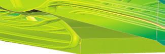
32 The temperature distribution is symmetric with a vertical mirror plane running between the two lower titanium bolts and running across the middle of the upper bolt. In this case, the model does not require much computing power and you can model the whole geometry. For more complex models, you can consider using symmetries in order to reduce the size of the model. The next Surface plot generated shows the current density in the device. 1 In the Model Builder, right-click Results and add a 3D Plot Group. Right-click 3D Plot Group 2 and add a Surface node. 2 In the Surface settings window under Expression, click the Replace Expression button. Select Joule Heating (Electric Currents)>Currents and charge>current density norm (jh.normj). jh-normj is the variable for the magnitude, or absolute value, of the current density vector. You can also enter jh-normj in the Expression field when you know the variable name. 3 Click the Plot button. The plot that displays in the Graphics window is almost uniform in color due to the high current density at the contact edges with the bolts. The next step is to manually change the color table range to visualize the current density distribution. 32 Thorough Example: The Busbar

33 4 On the Surface settings window under Range, select the Manual color range check box. Enter 1e6 in the Maximum field and replace the default. 5 Click the Plot button. The plot automatically updates in the Graphics window The resulting plot shows how the current takes the shortest path in the 90-degree bend in the busbar. Notice that the edges of the busbar outside of the bolts are hardly utilized for current conduction. Thorough Example: The Busbar 33

34 6 Click and drag the busbar in the Graphics window to view the back. Continue rotating the image to see the high current density around the contact surfaces of each of the bolts. Make sure to save the model. This version of the model, busbar.mph, is reused and renamed during the next set of tutorials. When you are done, click the Go to Default 3D View button and create a model thumbnail image. on the Graphics toolbar Creating Model Images from Plots With any solution, you can create an image to display in COMSOL when browsing for model files. After generating a plot select File>Save Model Thumbnail from the main menu. There are two other ways to create images from a plot. One is to click the Image Snapshot button in the Graphics toolbar to directly create an image. You can also add an Image node to a Report by right-clicking the plot group of interest. This completes the first part of the introduction to a multiphysics simulation. The next sections are designed to increase your understanding of the steps you implemented up to this point as well as to extend your simulation to include other 34 Thorough Example: The Busbar

35 relevant effects, like thermal expansion and fluid flow. These additional tutorial sections start on the following pages: Parameters, Functions, Variables, and Model Couplings on page 36 Material Properties and Libraries on page 41 Mesh Sequences on page 43 Adding Physics to a Model on page 45 Parameter Sweeps on page 64 Parallel Computing on page 71 Geometry Sequences on page 73 Thorough Example: The Busbar 35

36 Parameters, Functions, Variables, and Model Couplings This section explores working with Parameters, Functions, Variables, and Model Couplings. Global Definitions and Definitions contain functionality that help you to prepare model inputs and model couplings and to organize simulations. You have already used the functionality for adding Parameters to organize model inputs in Global Definitions on page 12. Functions, available as both Global Definitions and Definitions, contain a set of predefined functions that can be useful when setting up multiphysics simulations. For example, the Step function can create a smooth step function for defining different types of switches. To illustrate using functions, assume that you want to add a time dependent study to the busbar model by applying an electric potential across the busbar that goes from 0 V to 20 mv in 0.5 seconds. For this purpose, you could use a step function to be multiplied with the parameter Vtot. Add a function that goes smoothly from 0 to 1 in 0.5 seconds to find out how functions can be defined and verified. DEFINING FUNCTIONS For this section, you can continue working with the same model file created in the previous section. Locate and open the file busbar.mph if it is not already open on the COMSOL Desktop. 36 Parameters, Functions, Variables, and Model Couplings

37 1 Right-click the Global Definitions node and select Functions>Step. 2 In the Step settings window, enter 0.25 in the Location field to set the location of the middle of the step, where it has the value of Click Smoothing to expand the section and enter 0.5 in Size of the Transition zone to set the width of the smoothing interval. 4 Click the Plot button in the Step settings window. Parameters, Functions, Variables, and Model Couplings 37

38 If your plot matches the one below, this confirms that you have defined the function correctly. You can also add comments and rename the function to make it more descriptive. 5 Right-click the Step 1 node in the Model Builder and select Properties. 6 In the Properties window, enter any information you want. 38 Parameters, Functions, Variables, and Model Couplings

39 The Global Definitions and Definitions nodes can contain Variables, which are expressions of the dependent variables the variables that are solved for in a simulation. You can define global variables that can be used in several models. For the purpose of this exercise, assume that you want to introduce a second model to represent an electric device connected to the busbar through the titanium bolts. A first step would be to rename Model 1 to specify that it represents the busbar. 1 Right-click the Model 1 node and select Rename (or press F2). 2 In the Rename Model window, enter Busbar. Click OK and save the model. DEFINING MODEL COUPLINGS The next steps are for information only and you do not need to reproduce them unless you want to. Click the Definitions node under Busbar (mod1) to introduce a Model Coupling that integrates any Busbar (mod1) variable at the bolt boundaries facing the electric device. You can use this coupling to define a Variable in Global Definitions that calculates the total current. This variable is then globally accessible and could, for example, form a boundary condition for the current that is fed to the electric device in the Electric Device (mod2) node. The Model Couplings in Definitions have a wide range of use. The Average, Maximum, and Minimum model couplings have applications in generating results as well as in boundary conditions, sources, sinks, properties, or any other contribution to the model equations. The Probes are for monitoring the solution Parameters, Functions, Variables, and Model Couplings 39

40 progress. For instance, you can follow the solution in a critical point during a time-dependent simulation or at parameter value in a parametric study. You can also use Model Couplings to map variables from one face in a model to another (extrusion couplings) or to integrate a variable along curves and map from one entity to another (projection couplings). You can find an example of using the average operator in Parameter Sweeps on page 64. Also see Built-in Functions on page 114, for a list of available COMSOL functions. To learn more about working with definitions, in the Model Builder click the Definitions or Global Definitions node and press F1 to open the Dynamic Help window. This window displays help about the selected item in the COMSOL Desktop and provides links to the documentation. It could take up to a minute for the window to load the first time it is activated but the next time it will load quickly. 40 Parameters, Functions, Variables, and Model Couplings

41 Material Properties and Libraries Up to now, you have used the functionality in Materials to access the properties of copper and titanium in the busbar model. In Materials, you are also able to define your own materials and save them in your own material library. You can also add material properties to existing materials. In cases where you define properties that are functions of other variables, typically temperature, the plot functionality helps you to verify the property functions in the range of interest. First investigate how to add a property to an existing material. Assume that you want to add bulk modulus and shear modulus to the copper properties. CUSTOMIZING MATERIALS Locate and open the file busbar.mph if it is not already open on the COMSOL Desktop. 1 In the Model Builder, under Materials, click Copper. 2 In the Material settings window, the Materials Properties section contains a list of all the definable properties. Expand the Solid Mechanics>Linear Elastic Material section. Right-click Bulk Modulus and Shear Modulus and select Add to Material. This lets you define the bulk modulus and shear modulus for the copper in your model. Material Properties and Libraries 41

42 3 Locate the Material Contents section. Bulk modulus and Shear modulus rows are now available in the table. The warning sign indicates the values are not yet defined. To define the values, click the Value column. In the Bulk modulus row, enter 140e9 and in the Shear modulus row, enter 46e9. By adding these material properties, you have changed the Copper material. However, you cannot save this in the read-only Solid Mechanics material library. However, you can save it to your own material library. 4 In the Model Builder, right-click Copper and select Add Material to User Defined Library. 5 Right-click Materials and select Open Material Browser. In the Material Browser, right-click User Defined Library and select Rename Selected. 6 Enter My Materials in the Enter New Name dialog box. 42 Material Properties and Libraries

43 Mesh Sequences A model can contain different mesh sequences to generate meshes with different settings. These sequences can then be accessed by the study steps. In the study, you can select which mesh you would like to use in a particular simulation. In the busbar model, a second mesh node is added to create a mesh that is refined in the areas around the bolts and the bend. You do this by increasing the mesh resolution on curved surfaces. ADDING A MESH Locate and open the file busbar.mph (if it is not already open on the COMSOL Desktop). 1 In order to keep this model in a separate file for later use, from the main menu, select File>Save as and rename the model busbar_i.mph. 2 To add a second mesh node, right-click the Busbar (mod1) node and select Mesh. By adding another Mesh node, it creates a Meshes parent node that contains both Mesh 1 and Mesh 2. The Model 1 node was renamed to Busbar in a previous step. To display different combinations of node names, tags, and identifiers, select View>Model Builder Node Label and select an option from the list. 3 Click the Mesh 2 node. In the Mesh settings window under Mesh Settings, select User-controlled mesh as the Sequence type. A Size and Free Tetrahedral node are added under Mesh 2. 4 In the Model Builder, under Mesh 2, click Size. The asterisks in the upper-right corner indicate that the nodes are being edited. Mesh Sequences 43

44 5 In the Size settings window under Element Size, click the Custom button. 6 Under Element Size Parameters, enter: - mh/2 in the Maximum element size field - mh/2-mh/6 in the Minimum element size field in the Resolution of curvature field 7 Click the Build All button. Compare Mesh 1 and Mesh 2 by clicking the Mesh nodes. The mesh is updated in the Graphics window. An alternative for using many different meshes is to run a parametric sweep of the parameter for the maximum mesh size, mh, that was defined in the section Global Definitions on page 12. Mesh 1 Mesh 2 44 Mesh Sequences

45 Adding Physics to a Model COMSOL's distinguishing characteristics of adaptability and compatibility are prominently displayed when you add physics to an existing model. In this section, you will understand the ease with which this seemingly difficult task is performed. By following these directions, you can add structural mechanics and fluid flow to the busbar model. STRUCTURAL MECHANICS After completing the busbar Joule heating simulation, it is known that there is a temperature rise in the busbar. The next logical question to ask is: What kind of mechanical stress is induced by thermal expansion? To answer this question, COMSOL Multiphysics makes it easy for you to expand your model to include the physics associated with structural mechanics. To complete these steps, either the Structural Mechanics Module or the MEMS Module (which enhance the standard Solid Mechanics interface) is required. If you have a floating network license (FNL) or a class kit license (CKL) and your license file has been enabled for borrowing, you can borrow licenses from your license server. Select Options>Licenses from the main menu and then click Borrow. Select the licenses you want to borrow from the list and specify the number of days you want to keep them. Click OK. If you want to add cooling by fluid flow, or don t have the Structural Mechanics Module or MEMS Module, read this section and then go to, Fluid Flow on page 51. ADDING SOLID MECHANICS 1 Open the model busbar.mph that was created earlier. From the main menu, select File>Save as and rename the model busbar_ii.mph. 2 In the Model Builder, right-click the Busbar node and select Add Physics. Adding Physics to a Model 45

46 3 In the Model Wizard under Structural Mechanics, select Solid Mechanics. To add this interface, you can double-click it, right-click and select Add Selected, or click the Add Selected button. 4 Click the Finish button and save the file. You do not need to add any studies. When adding additional physics, you need to make sure that materials included in the Materials node have all the required properties for the selected physics. In this example, you already know that all properties are available for copper and titanium. You can start by adding the effect of thermal expansion to the structural analysis. 5 In the Model Builder under Solid Mechanics, right-click the Linear Elastic Material 1 node and from the domain level, select Thermal Expansion. A Thermal Expansion node is added to the Model Builder. With the Structural Mechanics Module, the Thermal Stress predefined multiphysics interface is also available to define thermal stresses and strains. 46 Adding Physics to a Model

47 6 In the Thermal Expansion settings window under Model Inputs, select Temperature (jh/jhm1) from the Temperature list. This is the temperature field from the Joule Heating interface (jh/jhm1) and couples the Joule heating effect to the thermal expansion of the busbar. Next, fix the busbar at the position of the titanium bolts. 7 In the Model Builder, right-click Solid Mechanics and from the boundary level, select Fixed Constraint. A node with the same name is added to the Model Builder. 8 Click the Fixed Constraint node. In the Graphics window, rotate the busbar to view the back. Click one of the bolts to highlight it and right-click to add the bolt to the Selection list. 9 Repeat this procedure for the remaining bolts to add boundaries 8, 15, and 43. Cross-check: Boundaries 8, 15, and 43. You can now update the Study to take the added effects into account. Adding Physics to a Model 47

48 RUNNING A STUDY SEQUENCE JOULE HEATING AND THERMAL EXPANSION The Joule heating effect is independent of the stresses and strains in the busbar, assuming small deformations and ignoring the effects of electric contact pressure. This means that you can run the simulation using the temperature as input to the structural analysis. In other words, the extended multiphysics problem is weakly coupled. As such, you can solve it in two separate study steps one for the strongly coupled Joule heating problem and a second one for the structural analysis. 1 In the Model Builder, right-click Study 1 and select Study Steps>Stationary to add a second stationary study step. When adding study steps you need to manually connect the correct physics with the correct study step. Start by removing the structural analysis from the first step. 2 Under Study 1, click the Step 1: Stationary node. 3 In the Stationary settings window, locate the Physics and Variables Selection. 4 In the Solid Mechanics (solid) row under Solve for, click to change the check mark to an to remove Solid Mechanics from Study 1. Now repeat these steps to remove Joule heating from the second study step. 48 Adding Physics to a Model

49 5 Under Study 1, click Step 2: Stationary 1. 6 Under Physics and Variables Selection, in the Joule Heating (jh) row under Solve for, click to change the check mark to an to remove Joule Heating from Step 2. 7 Right-click the Study 1 node and select Compute (or press F8) to solve the problem. After a few moments of computation a second plot group is added under Results in the Model Builder. Save the file busbarii.mph, which now includes the Solid Mechanics interface and the additional study step. RESULTING DEFORMATION Now add a displacement to the plot. 1 Under Results>3D Plot Group 2, click the Surface 1 node. Adding Physics to a Model 49

50 2 In the Surface settings window in the Expression section, click the Replace Expression button. From the context menu, select Solid Mechanics>Displacement>Total Displacements. You can also enter solid.disp in the Expression field. 3 Click Range to expand the section. Click to clear the Manual color range check box. The local displacement, due to thermal expansion, is displayed by COMSOL as a surface plot. Next add exaggerated deformation information. 4 In the Model Builder, under Results>3D Plot Group 2, right-click the Surface 1 node and add a Deformation. The plot automatically updates in the Graphics window. 5 Save the busbarii.mph file, which now includes a Surface plot with a Deformation. You can also plot the von Mises and principal stresses to assess the structural integrity of the busbar and the bolts. 50 Adding Physics to a Model

51 FLUID FLOW After analyzing the heat generated in the busbar and possibly the induced thermal stresses, you might want to investigate ways of cooling it by letting air flow over its surfaces. These steps do not require any additional modules. When you have the CFD Module or the Heat Transfer Module, the Conjugate Heat Transfer multiphysics interface is available. This automatically defines coupled heat transfer in solids and fluids including laminar or turbulent flow. Adding fluid flow to the Joule heating model forms a new multiphysics coupling. To simulate the flow domain, you need to create an air box around the busbar. You can do this manually by altering the geometry from your first model or by opening a Model Library file. Having loaded or created the geometry, now simulate the air flow as in this figure:. Air outlet Air inlet DEFINING INLET VELOCITY Start by adding a new parameter for the inlet flow velocity. 1 Select View>Model Library and navigate to COMSOL Multiphysics>Multiphysics>busbar_box. Double-click to open the model file, which Adding Physics to a Model 51

52 contains the geometry in addition to the steps completed up to the end of the section Customizing Materials on page Under Global Definitions, click the Parameters node. 3 In the Parameters settings window, click the last empty row in the Name column and enter Vin. Enter 1e-1[m/s] in the Expression column and a description of your choice in the Description column. 4 Select File>Save As and save the model with a new name, busbar_box_i.mph. ADDING AIR The next step is to add the material properties of air. 1 Select View>Material Browser. 2 In the Material Browser, expand the Built-In tree. Right-click Air and select Add Material to Model. Click the Material Browser tab and close it. 3 In the Model Builder under Materials, click the Air node. 52 Adding Physics to a Model

53 4 In the Graphics window, click the air box (Domain 1) to highlight it (in red) and right-click to add it to the Selection list (which changes the color to blue). Cross-check: Domain 1 ADDING FLUID FLOW Now add the physics of fluid flow. 1 In the Model Builder, right-click Model 1 and select Add Physics. 2 In the Add Physics tree, under Fluid Flow>Single-Phase Flow double-click Laminar Flow to add it to the Selected physics section. You do not need to add any more studies. Click the Finish button. Adding Physics to a Model 53

54 3 On the Graphics toolbar, click the Select Boundaries button and then the Wireframe rendering button to look inside the box. Now that you have added fluid flow to the model, you need to couple the heat transfer part of the Joule Heating interface to the fluid flow. 4 In the Model Builder, right-click Joule Heating. In the first section of the context menu, the domain level, select Heat Transfer in Solids>Heat Transfer in Fluids. 54 Adding Physics to a Model

55 5 In the Graphics window select the air box (Domain 1) and right-click to add it to the Selection list. Cross-check: Domain 1. Now couple fluid flow with heat transfer. 6 In the Heat Transfer in Fluids settings window under Model Inputs, select Velocity field (spf/fp1) from the Velocity field list. This identifies the flow field from the Laminar Flow interface and couples it to heat transfer. Now define the boundary conditions by specifying the inlet and outlet for the heat transfer in the fluid domain. 7 In the Model Builder, right-click Joule Heating. In the second section of the context menu, the boundary section, select Heat Transfer in Solids>Temperature. A Temperature node is added to the Model Builder Adding Physics to a Model 55

56 8 In the Graphics window, click the inlet boundary, Boundary 2, and right-click to add it to the Selection list. This sets the inlet temperature to 293 K, the default setting. Continue by defining the outlet. Cross-check: Boundary 2. 9 In the Model Builder, right-click Joule Heating. At the boundary level, select Heat Transfer in Solids>Outflow. An Outflow node is added to the Model Builder 56 Adding Physics to a Model

57 10 In the Graphics window, click the outlet boundary, Boundary 5, and right-click to add it to the Selection list. Cross-check: Boundary 5. The settings for the busbar, the bolts, and the Electric Potential 1 and Ground 1 boundaries have retained the correct selection, even though you added the box geometry for the air domain. To confirm this, click the Electric Potential 1 and the Ground 1 nodes in the Model Builder to verify that they have the correct boundary selection. Continue with the flow settings. You need to indicate that fluid flow only takes place in the fluid domain and then set the inlet, outlet, and symmetry conditions. Adding Physics to a Model 57

58 1 In the Model Builder, click the Laminar Flow node. In the Laminar Flow settings window, click the Clear Selection button. 2 In the Graphics window click the air box (Domain 1) and right-click to add it to the Selection. It is good practice to verify that the Air material under the Materials node has all the properties that this multiphysics combination requires. In the Model Builder under Materials, click Air. In the Material settings window under Material Contents, verify that there are no missing properties, which are marked with a warning sign. The section Materials on page 17 has more information. Continue with the boundaries. 3 In the Model Builder, right-click Laminar Flow and at the boundary level select Inlet. An Inlet node is added to the Model Builder. 58 Adding Physics to a Model

59 4 In the Graphics window, select the inlet (Boundary 2) and right-click to add it to the Selection list. Cross-check: Boundary 2. 5 In the Inlet settings window under Velocity in the U 0 field, enter Vin to set the Normal inflow velocity. 6 Right-click Laminar Flow and at the boundary level select Outlet. In the Graphics window, select the outlet (Boundary 5) and right-click to add it to the Selection list. Cross-check: Boundary 5. The last step is to add symmetry boundaries. You can assume that the flow just outside of the faces of the channel is similar to the flow just inside these faces. This is correctly expressed by the symmetry condition. Adding Physics to a Model 59

60 7 Right-click Laminar Flow and select Symmetry. A Symmetry node is added to the sequence. 8 In the Graphics window, click one of the blue faces in the figure (Boundaries 1, 3, 4, or 48) and right-click each one to add all to the Selection list. Save the busbar_boxi.mph file, which now includes the Air material and Laminar Flow interface settings. Cross-check: Boundaries 1, 3, 4 and 48. When you know the boundaries, you can click the Paste button and enter the information. In this example, enter 1,3,4,48 in the Paste selection window. Click OK and the boundaries are automatically added to the Selection list. The next step is to change the mesh slightly. COARSENING THE MESH In order to get a quick solution, the mesh is changed slightly and made coarser. The current mesh settings would take a relatively long time to solve, and you can always refine it later. 1 In the Model Builder, expand the Mesh 1 node and click the Size node. 60 Adding Physics to a Model

61 2 In the Size settings window under Element Size, click the Predefined button and ensure that Normal is selected. 3 Click the Build All button. The geometry displays with a coarse mesh in the Graphics window. You can assume that the flow velocity is large enough to neglect the influence of the temperature increase in the flow field. It follows that you can solve for the flow field first and then solve for the temperature using the results from the flow field as input. This is implemented with a study sequence. Adding Physics to a Model 61

62 RUNNING A STUDY SEQUENCE FLUID FLOW AND JOULE HEATING When the flow field is solved before the temperature field, it yields a weakly coupled multiphysics problem. The study sequence described in this section automatically solves such a weak coupling. 1 In the Model Builder, right-click Study 1 and select Study Steps>Stationary to add a second stationary study step to the Model Builder. Next, the correct physics needs to be connected with the correct study step. Start by removing Joule heating from the first step. 2 Under Study 1, click Step 1: Stationary. 3 In the Stationary settings window locate the Physics and Variables Selection section. In the Joule Heating (jh) row, click to change the check mark to an in the Solve for column, removing Joule Heating (jh) from Study 1. 4 Repeat the step. Under Study 1 click Step 2: Stationary 1. Under Physics and Variables Selection, in the Laminar Flow (spf) row click in the Solve for column to change the check mark to an. 62 Adding Physics to a Model

63 5 Right-click the Study 1 node and select Compute (or press F8) to automatically create a new solver sequence that solves the two problems in sequence. 6 After the solution is complete, click the Transparency button on the Graphics toolbar to visualize the temperature field inside the box. The Temperature Surface plot that displays in the Graphics window shows the temperature in the busbar and in the surrounding box. You can also see that the temperature field is not smooth due to the relatively coarse mesh. A good strategy to get a smoother solution would be to refine the mesh to estimate the accuracy. 7 Save the busbar_box_i.mph file up to this point so you can return to this file if you want. The next steps use the original busbar.mph file. Adding Physics to a Model 63

64 Parameter Sweeps Sweeping a Geometric Parameter Often it is interesting to generate multiple instances of a design to meet specific constraints. For the busbar, a design goal might be to lower the operating temperature and a decrease in the current density achieves this. Since the current density depends on the geometry of the busbar, varying the width, wbb, should change the current density and, in turn, have some impact on the operating temperature. Run a parametric sweep on wbb to study this change. ADDING A PARAMETRIC SWEEP 1 Open the model file busbar.mph. In the Model Builder, right-click Study 1 and select Parametric Sweep. A Parametric Sweep node is added to the Model Builder sequence. 2 In the Parametric Sweep settings window, under the table, click the Add button. From the Parameter names list in the table, select wbb. 64 Parameter Sweeps

65 3 Enter a range of Parameter values to sweep the width of the busbar from 5 cm to 10 cm with 1 cm increments. There are different ways to enter this information: - Copy and paste or enter range(0.05,0.01,0.1) into the Parameter value list field. - Click the Range button and enter the values in the Range dialog box. In the Start field, enter 5e-2. In the Step field, enter 1e-2 and in the Stop field, enter 1e-1. - Click Browse to Load parameter values from a text file. Next an Average Model Coupling is created, which can later be used to calculate the average temperature in the busbar. 4 Under Model 1, right-click Definitions and select Model Couplings>Average. 5 In the Average settings window select All domains from the Selection list. This creates an operator called aveop1. The aveop1 is now available to calculate the average of any quantity defined on those domains. A little later this is used to calculate the average temperature, but it can also be used to calculate average electric potential, current density, and so forth. 6 Right-click Study 1 and select Compute to run the sweep. 7 Select File>Save As to save the model with a new name, busbar_iii.mph. Parameter Sweeps 65

66 PARAMETRIC SWEEP RESULTS A Temperature (jh) 1 node is added under Results. The plot that displays in the Graphics window after the parametric sweep shows the temperature in the wider busbar using the last parameter value, wbb=0.1 m (10 cm). The plot is uniform in color, so change the maximum color range. 1 Under the Temperature (jh) 1 node, click the Surface node. 2 In the Surface settings window, click Range to expand the section. Select the Manual color range check box. Enter in the Maximum field (replace the default) to plot wbb at 10 cm. 66 Parameter Sweeps

67 3 The Temperature (jh) 1 plot is updated in the Graphics window for wbb= 0.1 m (10 cm). Compare the wider busbar plot to the temperature for wbb=0.05 m (5 cm). 1 In the Model Builder, click the first Temperature (jh) node. 2 In the 3D Plot Group settings window, select Solution 2 from the Data set list. This data set contains the results from the parametric sweep. 3 In the Parameters value list, select 0.05 (which represents wbb=5 cm). Click the Plot button. Click the Zoom Extents button on the Graphics toolbar. Parameter Sweeps 67

68 The Temperature (jh) plot is updated for wbb= 0.05 m (5 cm). Like the wider busbar, the plot is uniform in color, so change the maximum color range. 1 Under the first Temperature (jh) node, click the Surface node. 2 In the Surface settings window, click Range to expand the section (if it is not already expanded). Select the Manual color range check box. 3 Enter 323 in the Maximum field (replace the default) to plot wbb at 5 cm. The Temperature (jh) plot is updated in the Graphics window for wbb= 0.05 m (5 cm). 68 Parameter Sweeps

69 Click the first and second Temperature plot nodes to compare the plots in the Graphics window. It shows that the maximum temperature decreases from 331 K to 318 K as the width of the busbar increases from 10 cm to 5 cm. ADDING MORE PLOTS To further analyze these results, you can plot the average temperature for each width. 1 Right-click Results and add a 1D Plot Group. Then right-click 1D Plot Group 4 and add a Global node to the Model Builder. 2 In the Global settings window, select Solution 2 from the Data set list (the parametric sweep results). Select From list as the Parameter selection (wbb). 3 Under y-axis Data, click the first row in the Expressions column and enter aveop1(t). You use a similar syntax to calculate the average of other quantities. 4 Click to expand the Title section. Select the Expression check box. Parameter Sweeps 69

70 5 Click the Plot button and save the busbar_iii.mph model with these additional plots that use the parametric sweep results. In the plot, the average temperature also decreases as the width increases. This indicates that the goal of a lower operating temperature would be fulfilled by using a wider busbar. Of course, this may also increase the total mass (and therefore the cost) of the busbar. This suggests an optimization problem for you to consider. The subject of parameter sweeps naturally raises the question of parallel processing; it would be efficient if all parameters were solved simultaneously. 70 Parameter Sweeps

71 Parallel Computing COMSOL supports most forms of parallel computing including shared memory parallelism (for example, multicore processors) and high performance computing (HPC) clusters. You can use clusters to solve a series of parameter steps for a model, one parameter per node, or you can solve a single large model using distributed memory. For maximum performance, the COMSOL cluster implementation can utilize shared-memory multicore processing on each node in combination with the MPI-based distributed memory model. This brings a major performance boost by making the most out of the computational power installed. ADDING A CLUSTER COMPUTING JOB Continue these steps using the busbar_iii.mph model created in Adding a Parametric Sweep on page 64. To run cluster simulations, you need to first enable the advanced options for the Job Configurations node. 1 Click the Show button on the Model Builder and select Advanced Study Options. 2 In the Model Builder, under Study 1, right-click Job Configurations and select Cluster Computing. Parallel Computing 71

72 The Cluster Computing settings window helps to manage the simulation either for running several instances of an identical parameterized model one parameter value per host or for running one parameter step in distributed mode. You choose the type of cluster job you want to do from the Cluster type list. COMSOL supports Windows Computer Cluster Server (WCCS) 2003, Windows HPC Server (HPCS) 2008, Open Grid Scheduler/ Grid Engine (OGS/GE), or Not distributed. To learn more about running COMSOL in parallel, see the COMSOL Installation and Operations Guide. 72 Parallel Computing

73 Geometry Sequences This section details how to create the busbar geometry using COMSOL s geometry tools. The step-by-step instructions take you through the construction of the geometry using parameters set up in Global Definitions. Using parameterized dimensions helps to produce what-if analyses and automatic geometric parametric sweeps. Follow the steps under the Model Wizard (to add the physics and study) and Global Definitions (to add the parameters) starting with Thorough Example: The Busbar on page 9. Then return to this section to learn about geometry modeling. The first step in the geometry sequence is to draw the profile of the busbar. 1 Under Model 1, right-click Geometry 1 and select Work Plane. In the Work Plane settings window: - Select xz-plane from the Plane list. - Click the Show Work Plane button on the settings toolbar. Continue by editing the axis and grid settings in Work Plane 1. 2 In the Model Builder, expand the View 2 node and click Axis. Geometry Sequences 73

74 3 In the Axis settings window: Under Axis: - In the x minimum and y minimum fields, enter -1e-2. Replace the defaults. - In the x minimum and y minimum fields, enter Replace the defaults. Under Grid: - Select the Manual Spacing check box. - In the x spacing and y spacing fields, enter 5e-3. 4 Click the Apply button on the toolbar. You can use interactive drawing to create a geometry using the drawing toolbar buttons while pointing and clicking in the Graphics window. You can also right-click the Plane Geometry node under Work Plane 1 to add geometry objects to the geometry sequence. Right-click the Geometry node to add geometry objects. Click the Plane Geometry node under a Work Plane node to open the interactive toolbar. In the next set of steps, a profile of the busbar is created. 74 Geometry Sequences

75 5 In the Model Builder under Work Plane 1, right-click Plane Geometry and select Rectangle. In the Rectangle settings window under Size enter: - L+2*tbb in the Width field in the Height field Click the Build Selected button. 6 Create a second rectangle. Under Work Plane 1, right-click Plane Geometry and select Rectangle. Under Size, enter: - L+tbb in the Width field tbb in the Height field Under Position, enter: - tbb in the yw field Click the Build Selected button. Use the Boolean Difference operation to subtract the second rectangle from the first one. 7 Under Work Plane 1, right-click Plane Geometry and select Boolean Operations>Difference. In the Graphics window, click r1 and right-click to add r1 to the Objects to add list in the Difference settings window. Note: To help select the geometry, you can display geometry labels in the Graphics window. In the Model Builder under Geometry 1>WorkPlane 1>Plane Geometry, click the View 2 node. Go to the View settings window and select the Show geometry labels check box. Geometry Sequences 75

76 8 In the Difference settings window, click the Activate selection button to the right of the Objects to subtract list. Then right-click to add r2 to the list. Click Build Selected. Note: Another way to select r2 in the Graphics window is to use the Selection List window. Select View>Selection List and in the Selection List settings window, click to highlight r2 (solid). Then right-click r2 (solid) in the list to add it to the Object to subtract list. After building the selected geometry, you should have a backward-facing, L-shaped profile. Continue by rounding the corners using fillets. 76 Geometry Sequences

77 9 Under Work Plane 1, right-click Plane Geometry and select Fillet. Add point 3 to add it to the Vertices to fillet list. There are different ways to add the points: - In the Graphics window, click point 3 (in the inner right corner), and right-click to add it to the Vertices to fillet list. - Select View>Selection List. In the Selection List window, click 3. The corresponding point is highlighted in the Graphics window. Click the Add to Selection button on the Fillet settings window, or right-click in the Selection List. 10 Enter tbb in the Radius field. Click Build Selected. This takes care of the inner corner. 11 For the outer corner, right-click Plane Geometry and select Fillet. 12 In the Graphics window, click point 6, the outer corner, and right-click to add it to the Vertices to fillet list. 13 Enter 2*tbb in the Radius field. Click Build Selected. Geometry Sequences 77

78 The result should match this figure: Next you extrude the work plane to create the 3D busbar geometry. 1 In the Model Builder, right-click Work Plane 1 and select Extrude. In the Extrude settings window, enter wbb in the Distances from Plane table (replace the default) to extrude to the width of the profile. The table allows you to enter several values in order to create sandwich structures with different layer materials. In this case, only one extruded layer is needed. 78 Geometry Sequences

79 2 Click Build Selected and then click the Zoom Extents button on the Graphics toolbar. Click the Save button and name the model busbar.mph (if you have not already done so). Next, create the titanium bolts by extruding two circles drawn in two work planes. 3 In the Model Builder, right-click Geometry 1 and add a Work Plane. A Work Plane 2 node is added. In the Work Plane settings window, under Work Plane, select Face parallel as the Plane type. Geometry Sequences 79

80 4 In the Graphics window, click face 8 (highlighted in the figure). Once this surface is highlighted in red, right-click anywhere in the Graphics window to add it to the Planar face list in the Work Plane settings window. Face number 8 is now highlighted in blue and the work plane is positioned on top of face number 8. Face 8 5 Click the Show Work Plane button to draw the first circle representing the position of the first bolt. Click the Zoom Extents button on the Graphics toolbar. 6 Under Work Plane 2, right-click Plane Geometry and select Circle. In the Circle settings window: - Under Size and Shape in the Radius field, enter rad_1. - Under Position, the xw and yw coordinates (0, 0) are already defined. Click Build Selected. Continue creating the bolt by adding an extrude operation. 80 Geometry Sequences

81 1 In the Model Builder, right-click Work Plane 2 and select Extrude. In the Extrude settings window, in the first row of the Distances from Work Plane table, enter -2*tbb to extrude the circle a distance equal to the thickness of the busbar. 2 Click the Build Selected button to create the cylindrical part of the titanium bolt that runs through the busbar. Draw the two remaining bolts. 3 Right-click Geometry 1 and select Work Plane. A Work Plane 3 node is added. In the Work Plane settings window, for Work Plane 3, select Face parallel as the Plane type. Geometry Sequences 81

82 4 In the Graphics window, click Face 6 (shown in the figure). When this surface is highlighted red, right-click anywhere in the Graphics window to add it to the Planar face list in the Work Plane settings window. 5 Click the Show Work Plane button on the Work Plane settings window and the Zoom Extents button on the Graphics toolbar to get a better view of the geometry. To parameterize the position of the two remaining bolts, add the circles that form the cross sections of the bolts. 6 Under Work Plane 3, right-click Plane Geometry and select Circle. In the Circle settings window: - Under Size and Shape, enter rad_1 in the Radius field. - Under Position, enter -L/2+1.5e-2 in the xw field and -wbb/4 in the yw field. Click Build Selected. Copy the circle that you just created to generate the third bolt in the busbar. 7 Under Work Plane 3, right-click Plane Geometry and select Transforms>Copy. 82 Geometry Sequences

83 8 In the Graphics window, click the circle c1 to highlight it. Right-click anywhere in the Graphics window and add the circle to the Input object list in the Copy settings window. 9 In the Copy settings window under Displacement, enter wbb/2 in the yw field. 10 Click Build Selected. Your geometry, as shown in the workplane, should match this figure so far. Continue by extruding the circles. 11 In the Model Builder, right-click Work Plane 3 and select Extrude. In the Extrude settings window, in the first row of the Distances from Work Plane table, enter -2*tbb (replace the default). Click Build All. Geometry Sequences 83

84 The geometry and its corresponding geometry sequence should match the figure. Click the Save button and name the model busbar.mph. To continue with the busbar tutorial, return to the section Global Definitions on page 12 to add the parameters to the busbar.mph model file. 84 Geometry Sequences

85 Easy Example: The Wrench Torquing a Wrench Working with hand tools gives you a practical introduction to basics of engineering. At some point in your life It is likely you have tightened a bolt using a wrench. This exercise takes you through a model that analyzes this basic task, going into detail about the associated geometric tolerances, torque specs, and the intrinsic contact problem. In principle, a bolt replaces the need for external fastening by providing an internal clamping force via pretension. The tensile stress in a bolt is produced when it is torqued into a matching threaded hole or nut. The magnitude of this stress depends on many factors, such as material selection, assembly configuration, and lubrication. Control of these parameters becomes the focus of much engineering effort, especially in critical applications such as automotive engines, brakes, aircraft, and structural installations. The following model presents both a bolt and a wrench at the moment of installation. The following tutorial is a short introduction to using COMSOL Multiphysics and it includes the basics of COMSOL Multiphysics. Start by opening the Model Wizard and add a physics and a study, then import a geometry, open the Material Browser to add a material and examine the material properties. The other key steps to creating a model are then explored by defining a parameter, defining the boundary conditions, selecting geometric entities in the Graphics window, defining the Mesh and Study nodes, and finally examining the resulting plots. If you prefer to practice with a more advanced model, read this section to familiarize yourself with some of the key features, and then go to the tutorial Thorough Example: The Busbar on page 9. Easy Example: The Wrench 85

86 MODEL WIZARD 1 Open the Model Wizard. To open the Model Wizard, double-click the COMSOL icon on the desktop. Or when COMSOL is already open: - Click the New button on the main toolbar - Select File>New from the main menu - Right-click the root node and select Add Model 2 In the Select Space Dimension window that opens, the 3D button is selected by default. Click Next. 3 In Add Physics, select Structural Mechanics > Solid Mechanics (solid). Double-click or right-click to add it to the Selected physics section. Click Next. Another way to open the Add Physics window is to right-click the Model node and select Add Physics. 4 Click Stationary under Preset Studies. Click the Finish button. Preset Studies are studies that have solver and equation settings adapted to the selected physics, in this example, Joule heating. Any selection from the Custom Studies branch needs manual fine-tuning. 86 Easy Example: The Wrench

87 GEOMETRY This tutorial uses a predefined geometry. To learn how to build your own geometry for the busbar model, see Geometry Sequences on page 73. File Locations For both the wrench and busbar tutorials in this guide, you can load predefined geometry or parameter files into COMSOL instead of manually adding the information. The location of the text and model files used in this exercise varies based on the software installation. For example, if the installation is on your hard drive, the file path might be similar to C:\Program Files\COMSOL43\models\. 1 Under Model 1, right-click Geometry 1 and select Import. 2 In the Import settings window, from the Geometry import list, select COMSOL Multiphysics file. 3 Click Browse and locate the file wrench.mphbin in the Model Library folder COMSOL_Multiphysics/Structural_Mechanics. Double-click to add or click Open. Easy Example: The Wrench 87

88 4 Click Import to display the geometry in the Graphics window. Rotate: Left-click and drag Pan: Right-click and drag 5 Click the Save button on the main toolbar or select File>Save and name the model wrench.mph. Click the wrench geometry in the Graphics window and experiment with moving it around. As you click and right-click the geometry, it changes color. Click the Zoom In, Zoom Out, Go to Default 3D View, Zoom Extents, and Transparency buttons on the toolbar to see what happens to the geometry. - To rotate the busbar, left-click and drag it in the Graphics window - To move it, right-click and drag - To zoom in and out, center-click (and hold) and drag Also see Keyboard Shortcuts on page 107 and Working with 3D Geometry in the Graphics Window on page 105 for additional information. 88 Easy Example: The Wrench

89 MATERIALS The Materials node stores the material properties for all physics and all domains in a Model node. The chosen bolt material and tool steel are important characteristics of this contact problem. Here is how to choose them in COMSOL. 1 Open the Material Browser. To open the Material Browser you can: - Right-click Materials in the Model Builder and select Open Material Browser - Select View>Material Browser 2 In the Material Browser, under Materials, expand the Built-In folder. Scroll down to find Structural Steel, right-click and select Add Material to Model. 3 Examine the Material Contents section to see how COMSOL categorizes available material information with respect to what the active physics requires. Easy Example: The Wrench 89

90 Also see the busbar tutorial sections Materials on page 17 and Customizing Materials on page 41 to learn more about working with the Material Browser. GLOBAL DEFINITIONS Parameters 1 In the Model Builder, right-click Global Definitions and choose Parameters. 2 Go to the Parameters settings window. Under Parameters in the Parameters table (or under the table in the fields), enter these settings: - In the Name column or field, enter F. - In the Expression column or field, enter 150[N]. The Value column is automatically updated based on the expression entered. - In the Description column or field, enter Applied force. In the busbar tutorial, the section Global Definitions on page 12 and Parameters, Functions, Variables, and Model Couplings on page 36 shows you more about working with parameters. So far, you have added the physics and study, imported a geometry, added the material and defined one parameter. The Model Builder node sequence should match the figure. The default feature nodes under Solid Mechanics are indicated by a D in the upper left corner of the node. 90 Easy Example: The Wrench

91 DOMAIN PHYSICS AND BOUNDARY CONDITIONS With the geometry and materials defined, you are now ready to revisit the governing physics introduced in the Model Wizard section. 1 In the Model Builder, right-click Solid Mechanics (solid) and at the boundary level, select Fixed Constraint. 2 In the Graphics window, rotate the geometry by left-clicking and dragging into the position shown. Then left-click the cut-face of the partially modeled bolt (which turns the boundary red) and right-click to select it (which turns the boundary blue). Also see Working with 3D Geometry in the Graphics Window on page Click the Go to Default 3D View button on the Graphics toolbar to restore the geometry to the default view. Cross-check: Boundary 35. Easy Example: The Wrench 91

92 4 In the Model Builder, right-click Solid Mechanics (solid) and at the boundary level, select Boundary Load. A Boundary Load node is added to the Model Builder sequence. 5 In the Graphics window, click the Zoom Box button on the toolbar and drag the mouse to highlight the area shown in the figure to the right. Release the mouse button. 6 Select the top socket face (Boundary 111) by left-clicking to highlight the boundary in red and right-clicking it to highlight it in blue and add it to the Selection list. Cross-check: Boundary In the Boundary Load settings window, under Force, select Total force as the Load type and enter -F. The negative sign indicates the negative z direction (downward). 92 Easy Example: The Wrench

93 MESH Because the geometry contains small edges and faces, reduce the size of the minimum element. 1 In the Model Builder, under Model 1 click Mesh 1. In the Mesh settings window, under Mesh settings, from the Sequence type list select User-controlled mesh. 2 Under Mesh 1 click the Size node. Note: The asterisks in the upper-right corner of the mesh nodes are dynamic feedback icons indicating that these nodes are being edited. 3 In the Size settings window under Element Size, click the Custom button. 4 Under Element Size Parameters, in the Minimum element size field, enter Click the Build All button on the Size settings window toolbar. After a few seconds, the mesh builds. Zoom in to the mesh and have a look at the distribution. Easy Example: The Wrench 93

94 STUDY The following steps are needed to set up an iterative solver. By using such a solver, you can significantly reduce the memory amount needed for the calculations. If your computer has more than 2 GB of memory, you can skip these steps and go directly to step 6 to compute the solution. 1 In the Model Builder, right-click Study 1 and choose Show Default Solver. 2 Expand the Study 1>Solver Configurations>Solver 1> node. 3 Right-click Stationary Solver 1 and choose Iterative. 4 Right-click Iterative 1 and choose Multigrid. 5 Right-click Study 1 and select Compute (or press F8). After a few seconds of computation time, the default plot is displayed in the Graphics window. You can find other useful information about the computation by clicking the Messages and Log tabs under the Graphics window to see the kind of information available to you. These windows can also be opened from the main View menu. DISPLAYING RESULTS The default von Mises stress is displayed in the Graphics window in a Surface plot with the displacement visualized using a Deformation subnode. Change the default unit (N/m 2 ) to the more suitable MPa. 94 Easy Example: The Wrench

95 1 In the Model Builder, expand the Results>Stress (solid) node, then click Surface 1. 2 In the settings window under Expression, from the Unit list select MPa (or enter MPa in the field). 3 Click the Plot button and the Zoom Extents button on the Graphics toolbar. The plot is regenerated with the updated unit and shows the von Mises stress distribution in the bolt and wrench under an applied vertical load. Now determine the location of greatest tension by plotting the principal strain field. Easy Example: The Wrench 95

96 PLOTTING THE PRINCIPAL STRAIN FIELD 1 Right-click the Results node and add a 3D Plot Group. 2 Right-click the 3D Plot Group 2 node and select Surface. 3 In the Surface settings window click the Replace Expression button and select Solid Mechanics>Strain>Principal strains> First principal strain (solid.ep1). When you know the variable name, as in this exercise, you can also enter solid.ep1 in the Expression field. 4 Click the Plot button. 5 In the Model Builder, click 3D Plot Group 2. Press F2 and in the Rename 3D Plot Group window, enter First Principal Strain. Click OK. 96 Easy Example: The Wrench

97 Notice that the maximum principal strain is lower than 2%, a result that satisfies the small strain assumption. This concludes the wrench tutorial. The following sections provide you with some additional concepts to get you started with modeling in COMSOL. Easy Example: The Wrench 97

98 COMSOL Multiphysics Additional Concepts The next sections provide some additional concepts about working in COMSOL Multiphysics, including an explanation about geometric entities and what node types are shown to help you visualize your modeling. A introduction to the Model Builder and some of the terminology and navigation tools is included in the key to the table, and the last section describes the COMSOL Multiphysics file types. About Geometric Entities and the Different Node Types The Model Builder has many types of nodes to help you visualize the model structure. After you click the Finish button ( ) on the Model Wizard window, a Model node is added to the Model Builder based on the space dimension selected in the first step. The Model node has different images for each node s space dimension. The nodes under the physics also indicate several things the space dimension of the geometric entity applied to the node (at the domain, boundary, edge, or point level), and other useful pieces of information, such as whether it is a default node or a pair. The geometric entity name varies based on space dimension, but the nodes clearly indicate the type of node you are working with. Also see Working with 3D Geometry in the Graphics Window for some more information about geometric entities and how to move and rotate geometry in the Graphics window. GEOMETRIC ENTITY NAMES IN DIFFERENT SPACE DIMENSIONS ENTITY DIMENSION NAME IN 3D NAME IN 2D NAME IN 1D NAME IN 0D 3D domain 2D boundary domain 1D edge boundary domain 0D vertex vertex boundary domain SPACE DIMENSION DOMAIN BOUNDARY EDGE POINT DEFAULT NODE EXAMPLE 3D PAIR 2D 2D axisymmetric 1D 98 COMSOL Multiphysics Additional Concepts

99 SPACE DIMENSION DOMAIN BOUNDARY EDGE POINT DEFAULT NODE EXAMPLE 1D axisymmetric PAIR 0D not applicable Additional node types include a whether it is an exclusive node, for example, a contributing node, if the node is overridden by another node, or if it overrides other nodes. E XCLUSIVE NODES The use of an exclusive node means that only one node can be active for a given selection. That is, if you add another exclusive node (for example, an identical feature node) with the same selection, the first exclusive node is overridden and thus has no effect. Typical exclusive nodes include model equations, initial values, and boundary conditions that are constraints, such as prescribed values for displacements, temperatures, pressures, and so on, including special variants of these such as ground conditions in electromagnetics and fixed constraints in structural mechanics. Also some boundary conditions that are not constraints but have a definitive meaning are exclusive nodes for example, electric insulation, thermal insulation, and no-flow conditions. O VERRIDDEN AND OVERRIDING NODES Depending on the selections for each node, an exclusive node can override another node partially. Nodes are exclusive only within their specific physics. When a node is selected in the Model Builder tree, nodes that are overridden by the selected node are indicated by this icon ( ), and nodes that override the selected node are indicated by this icon ( ). C ONTRIBUTING NODES A contributing node ( ) means you can have several of these nodes with the same selection the software adds these together when evaluating the model. Typical contribution nodes are loads, fluxes, and source terms, where you can have more than one of each type that is active on the same domain or boundary, for example. COMSOL Multiphysics Additional Concepts 99

100 O THER NODE TYPES Other indicators include show the status of nodes (is the node current, being built or edited, for example) or alert you to problems (error and warning nodes). TYPE EXAMPLE DESCRIPTION Current node A current node is used for Geometry and Meshing nodes and indicates that the feature or sequence of steps has been built. It is a green line on the left and upper edges of the node. Current node, but not built Editing, or in process of editing, a node Warning Error (indicator) Error (node) This node is current, but not yet built, for example, on a Geometry node. It is a brown line on the left and upper edges of the node. This example is also displaying the asterisk indicating the node is being edited. An edited node has a blue asterisk (star) in the upper right corner of the node, for example, on a Mesh node. The asterisk also appears on plot nodes when the plot has not been updated to reflect changes in the data or settings (for example, after re-solving), A warning does not prevent the completion of a task but it might affect the accuracy or other aspects of the model. When there is a yellow triangle with an explanation mark in the lower right corner of the node, a warning message displays. Other warnings typically appear in the Log window. An error prevents the program from completing a task. For many error types, a red X is added to the lower right-hand corner of the node where the error is occurring. For example, on a Material node, to indicate that information is missing. An error prevents the program from completing a task. This is an error subnode which contains an error message that generally provide additional information. It is a node with an X in a red circle, for example, under a Solver node. P LOT AND PLOT GROUP NODES The plot groups and plots also indicate the space dimension and the type of plot being used. There are too many plot types to list here, but the key is that all the 1D and polar plots selected from 1D Plot Group and Polar Plot Group nodes are green, all the 2D plots selected from the 2D Plot Group node are pink, and all the 3D plots selected from the 3D Plot Group node are blue, as shown in this figure. 100 COMSOL Multiphysics Additional Concepts