Human Identification Based on Three- Dimensional Ear and Face Models

Transcription

1 University of Miami Scholarly Repository Open Access Dissertations Electronic Theses and Dissertations Human Identification Based on Three- Dimensional Ear and Face Models Steven Cadavid University of Miami, Follow this and additional works at: Recommended Citation Cadavid, Steven, "Human Identification Based on Three-Dimensional Ear and Face Models" (2011). Open Access Dissertations This Open access is brought to you for free and open access by the Electronic Theses and Dissertations at Scholarly Repository. It has been accepted for inclusion in Open Access Dissertations by an authorized administrator of Scholarly Repository. For more information, please contact

2

3 UNIVERSITY OF MIAMI HUMAN IDENTIFICATION BASED ON THREE-DIMENSIONAL EAR AND FACE MODELS By Steven Cadavid A DISSERTATION Submitted to the Faculty of the University of Miami in partial fulfillment of the requirements for the Degree of Doctor of Philosophy Coral Gables, Florida May 2011

4 c 2011 Steven Cadavid All Rights Reserved

5 UNIVERSITY OF MIAMI A dissertation submitted in partial fulfillment of the requirements for the degree of Doctor of Philosophy HUMAN IDENTIFICATION BASED ON THREE-DIMENSIONAL EAR AND FACE MODELS Steven Cadavid Approved: Mohamed Abdel-Mottaleb, Ph.D. Professor of Electrical and Computer Engineering Terri A. Scandura, Ph.D. Dean of the Graduate School Kamal Premaratne, Ph.D. Professor of Electrical and Computer Engineering Akmal A. Younis, Ph.D. Associate Professor of Electrical and Computer Engineering Anil K. Jain, Ph.D. Distinguished Professor of Computer Science and Engineering Michigan State University Hanqi Zhuang, Ph.D. Professor of Computer & Electrical Engineering and Computer Science Florida Atlantic University

6 CADAVID, STEVEN (Ph.D., Electrical and Computer Engineering) Human Identification Based on Three-Dimensional (May 2011) Ear and Face Models Abstract of a dissertation at the University of Miami. Dissertation supervised by Professor Mohamed Abdel-Mottaleb. No. of page in text. (137) We propose three biometric systems for performing 1) Multi-modal Three- Dimensional (3D) ear + Two-Dimensional (2D) face recognition, 2) 3D face recognition, and 3) hybrid 3D ear recognition combining local and holistic features. For the 3D ear component of the multi-modal system, uncalibrated video sequences are utilized to recover the 3D ear structure of each subject within a database. For a given subject, a series of frames is extracted from a video sequence and the Region-of-Interest (ROI) in each frame is independently reconstructed in 3D using Shape from Shading (SFS). A fidelity measure is then employed to determine the model that most accurately represents the 3D structure of the subject s ear. Shape matching between a probe and gallery ear model is performed using the Iterative Closest Point (ICP) algorithm. For the 2D face component, a set of facial landmarks is extracted from frontal facial images using the Active Shape Model (ASM) technique. Then, the responses of the facial images to a series of Gabor filters at the locations of the facial landmarks are calculated. The Gabor features are stored in the database as the face model for recognition. Match-score level fusion is employed to combine the match scores obtained from both the ear and face modalities. The aim of the proposed system is to demonstrate the superior performance that can be achieved by combining the 3D ear and 2D face modalities over either modality employed independently. For the 3D face recognition system, we employ an Adaboost algorithm to build

7 a classifier based on geodesic distance features. Firstly, a generic face model is finely conformed to each face model contained within a 3D face dataset. Secondly, the geodesic distance between anatomical point pairs are computed across each conformed generic model using the Fast Marching Method. The Adaboost algorithm then generates a strong classifier based on a collection of geodesic distances that are most discriminative for face recognition. The identification and verification performances of three Adaboost algorithms, namely, the original Adaboost algorithm proposed by Freund and Schapire, and two variants the Gentle and Modest Adaboost algorithms are compared. For the hybrid 3D ear recognition system, we propose a method to combine local and holistic ear surface features in a computationally efficient manner. The system is comprised of four primary components, namely, 1) ear image segmentation, 2) local feature extraction and matching, 3) holistic feature extraction and matching, and 4) a fusion framework combining local and holistic features at the match score level. For the segmentation component, we employ our method proposed in [111], to localize a rectangular region containing the ear. For the local feature extraction and representation component, we extend the Histogram of Categorized Shapes (HCS) feature descriptor, proposed in [111], to an object-centered 3D shape descriptor, termed Surface Patch Histogram of Indexed Shapes (SPHIS), for surface patch representation and matching. For the holistic matching component, we introduce a voxelization scheme for holistic ear representation from which an efficient, element-wise comparison of gallery-probe model pairs can be made. The match scores obtained from both the local and holistic matching components are fused to generate the final match scores. Experimental results conducted on the University of Notre Dame (UND) collection J2 dataset demonstrate that the

8 proposed approach outperforms state-of-the-art 3D ear biometric systems in both accuracy and efficiency.

9 TABLE OF CONTENTS List of Figures vii List of Tables x 1 Introduction Related Work Three-Dimensional (3D) Ear Recognition D Face Recognition D Ear Modeling and Recognition from Video Sequences using Shape from Shading System Approach Video Frames Independently Reconstructed in 3D using Shape from Shading (SFS) Linear Shape from Shading D Model Registration Similarity Accumulator D Model Selection Recognition Process Experimental Setup Experimental Results Conclusion iii

10 3 Multi modal Ear and Face Modeling and Recognition Summary Related Work in Multi-modal Ear and Face Recognition Two-Dimensional (2D) Face Recognition Using Gabor Features Data Fusion Experiments and Results Conclusions and Future Work Determining Discriminative Anatomical Point Pairings using AdaBoosted Geodesic Distances for 3D Face Recognition Motivation Related Work in the Application of Geodesic Distance Features to 3D Face Recognition Methods that Explicitly Compare Geodesic Distances Methods that use Geodesic Distances to Derive Expression- Invariant Facial Representations Contribution Construction of Dense Correspondences Global Mapping Local Conformation An Extension of the Bentley-Ottman Algorithm Generic Model Conformation Computing Geodesic Distances Between Anatomical Point Pairs The Fast Marching Method on Triangulated Domains Implementation Learning the Most Discriminant Geodesic Distances Between Anatomical Point Pairs by AdaBoost iv

11 4.5.1 Real Adaboost Gentle Adaboost Modest Adaboost Classification and Regression Trees Intra-Class and Inter-Class Space Implementation Experimental Setup Experimental Results Conclusion A Computationally Efficient Approach to 3D Ear Recognition Employing Local and Holistic Features Overview Local Feature Representation Preprocessing Histogram of Indexed Shapes (HIS) Feature Descriptor Shape Index and Curvedness HIS Descriptor D Keypoint Detection Local Feature Representation Surface Patch Histogram of Indexed Shape(SPHIS) Descriptor Local Surface Matching Engine Holistic Feature Extraction Preprocessing Surface Voxelization Binary Voxelization Holistic Surface Matching Engine v

12 5.4 Fusion Experimental Results Identification Scenario Verification Scenario Training of the Data Fusion Parameters Comparison with Other Methods Similarity-based Classification Similarities as Features Similarities as Kernels Similarity-Based Weighted Nearest Neighbors Experimental Results Conclusion and Future Work Concluding Remarks Conclusion Differential Geometry of Surfaces Principal Curvature Surface Normals Active Shape Model Bibliography vi

13 LIST OF FIGURES 2.1 Ear segmentation. a) Original image, b) filtering using mathematical morphology, c) binary thresholding using K-means clustering, d) connected components labeling, and e) detected ear region Effect of smoothing on surface reconstruction. a) Without filtering and b) With filtering Sample ear images (row 1) and their corresponding 3D reconstructions (row 2) taken from the database D reconstruction and global registration Similarity Components. a) Maximum curvature, b) minimum curvature, and c) surface normals Constructing the search window Similarity accumulator Mean CMC curves of different frames A sample ear image sequence at varying degrees of off-axis pose. a) 0, b) 5, c) 10, d) 15, e) 20, and f) Partially-segmented ear model. a) Partially-segmented ear region and b) resulting 3D ear model Extracted landmark points. 75 landmark points are extracted by the ASM method Sample face (row 1) and ear (row 2) image pairs taken from the database CMC curves of the 2D ear recognition, 3D face recognition, and the fusion of the two modalities ROC curves for the 2D ear recognition, 3D face recognition, and the fusion of the two modalities Global mapping. (a) The generic (left) and scanned (right) models prior to the global mapping. (b) The TPS method coarsely registers the two models based on a set of control points Local mapping. (a) The generic and (b) scanned models are sub-divided into corresponding regions based on their respective control points. (c) The similarity values of the correspondences established between the generic model and a sample scanned model vii

14 4.3 Surface conformation results under different correspondence configurations. (a) Ideal correspondence configuration and (c) resulting surface conformation. (b) Intersecting correspondence configuration that will lead to (d) the surface folding over itself (a) The generic model prior to global and local mapping. (b) A sample scanned model. (c) The two models are finely registered based on a dense set of correspondences. (d) The conformed generic model after the local mapping (a) The six-connected neighborhood of vertices. (b) Geodesic distances from the nose tip to several surrounding vertices. The surface color represents the distance field (a) Source vertices located on the index map. (b & e) The projection of source vertices from the index map onto a sample 3D face model. (d) Destination vertices associated with a given source vertex (nose tip) located on the index map. (c & f) The projection of destination vertices from the index map onto a sample 3D face model The CMC curves based on the match scores produced by the Adaboost algorithms The ROC curves in semi-log form based on the match scores produced by the Adaboost algorithms Rank-one identification rate of the Gentle Adaboost classifier as a function of the number of weak classifiers selected The weighted distribution of geodesic distance features selected by the Gentle Adaboost algorithm; dark blue and dark red indicating maximal and minimal contributions, respectively System overview Keypoint detection. (a) A surface. (b) Candidate keypoints. (c) PCA applied to keypoint-centered surface patches. (d) Final keypoints Keypoint detection repeatability of the 3D ear SPHIS feature extraction. First row from left to right: the shape index map, the 3D ear with a sphere centered at a keypoint that is used to cut the surface patch for SPHIS feature generation, and the curvedness map. Second row from left to right: A surface patch cropped by the sphere with the keypoint marked, and four sub-surface patches dividing the cropped surface patch with points colored differently for each subsurface patch. Third row: the four sub-surface patches shown with the keypoint. Fourth row: the HIS descriptors with 16 bins extracted from the corresponding sub-surface patches. Last row: The final SPHIS feature descriptor An example of finding feature correspondences for a pair of gallery and viii

15 probe ears from the same subject. (a) Keypoints detected on the ears. (b) True feature correspondences recovered by the local surface matching engine Binary voxelization. a) A sample ear model inscribed in a grid comprised of cubed voxels with dimensions of size 8.0mm. b) The voxelized model with voxels of dimension size 8.0mm c) The sample ear model in a) inscribed in a grid comprised of cubed voxels with dimensions of size 4.0. d) The voxelized model with voxels of dimension size 4.0mm. A cube present within a voxel denotes an associated value of 1 and 0, otherwise CMC curve Verification rate vs. FAR curve A1.1 Principal curvature ix

16 LIST OF TABLES 2.1 Experimental results for varying poses EER comparison of different ear poses Performance comparison to other 3D ear biometric systems Different techniques were used to fuse the normalized match scores of the 3D ear and 2D face modalities Performance comparison to other 3D face recognition systems tested on the FRGC v1.0 database D collection Nine shape categories are obtained by quantizing the shape index value range Recognition performances of different binary voxel sizes Experimentation datasets derived from the UND database The rank-one recognition rates of the identification experiments The EERs and verification rates of the verification experiments Identification performance comparison on the UND Database J2 Collection (415 subjects, 1386 probes) Verification performance comparison on the UND Database J2 Collection (415 subjects, 1386 probes) Identification performance comparison on a single-model probe and gallery set Verification performance comparison on a single-model probe and gallery set Similarity-based classification results on the All vs. All dataset pairing Similarity-based classification results on the All vs. All dataset pairing for different values of k x

17 Chapter One Introduction Confirming a person s identity is an important element of any security system. Biometrics the use of unique human characteristics to positively identify a person offers the most reliable technique to answer this enormous need in society today. But the search continues for the best approach to biometric identity confirmation that offers the combination of total reliability, speed and ease of use. Ear and face biometrics may offer that solution. The face possesses several inherent characteristics that render it a preferred biometric. An advantage of employing the face as a biometric is that its acquisition is non-intrusive, meaning an individual can be scanned and their identity confirmed without the subject actively engaging the device, as is required to use an iris or fingerprint. Additionally, the face contains prominent features, such as the eye and mouth corners, which can be robustly localized using their distinctive shape and texture properties. These qualities have enticed researchers and has inspired more than three decades of work in the area of face recognition [46]. The majority of the work in face recognition has been conducted in the 2D domain. 2D face recognition methods have been broadly divided into three categories holistic, feature-based, and hybrid methods which are based on guidelines suggested by psychological studies of how humans utilize holistic and local features [109]. Holistic methods treat facial images as vectors of a multidimensional Euclidean space and use standard dimensionality reduction techniques to construct a representation of the face. One of the most widely used representations of the 1

18 2 facial region is based on Principal Components Analysis (PCA) and is known as the Eigen-Faces approach, proposed in [92]. In contrast, feature-based methods utilize the locations and statistics (geometric and/or appearance) of local facial features to construct a classifier for face recognition. Hybrid methods attempt to emulate the human visual perception system by employing both holistic and local features to discriminate between subjects. One can argue that hybrid methods could potentially offer the best of both holistic and feature-based methods. Despite the efforts made in 2D face recognition, it is not yet ready for real world applications as a uni-modal biometric system. Most systems perform well only under constrained conditions (i.e., homogeneous lighting conditions), even requiring that the subjects be highly cooperative (maintaining frontal head pose and neutral facial expression) during acquisition. Furthermore, it has been observed that the variations between the images of the same face due to illumination and viewing direction are often larger than those caused by changes in face identity [2]. The introduction of the 3D face modality alleviates some of these challenges by introducing a depth dimension that is invariant to both lighting conditions and head pose. 3D face recognition has the potential to achieve better performance than its 2D counterpart by exploiting the 3D geometrical properties of rigid features on the facial surface. Advances in 3D range scanning technology has enabled the simultaneous capture of aligned 2D color images and 3D depth images. Consequently, 3D facial data can be used to improve the accuracy of 2D image based recognition by synthesizing the 2D facial region into a normalized frontal pose. Additionally, 3D data eliminates ambiguity in the size of the facial region usually present in the 2D modality. Unlike 2D images, where the unspecified distance between the

19 3 individual and the camera can lead to differently sized facial regions, 3D facial data is metrically accurate. Like face recognition, recent work in ear biometrics has demonstrated the promising potential of the ear as a viable passive biometric marker. Yet ears may be much more reliable than a face, which research has shown is prone to erroneous identification because of the ability of a subject to change their facial expression or otherwise manipulate their visage. The ear, initial case studies have suggested, has sufficient unique features to allow a positive and passive identification of a subject [43]. Furthermore, the ear is known to maintain a consistent structure throughout a subject s lifespan [43]. Medical literature has shown proportional ear growth after the first four months of birth [43]. However, there are drawbacks inherent to ear biometrics. For instance, the ear is prone to self-occlusion because of its prominent ridges. For this reason, ear recognition systems are typically sensitive to ear pose. Additionally, a drawback that poses difficulty to the feature extraction process is occlusion due to hair or jewelery (e.g., earrings or the arm of a pair of eyeglasses). It is important to justify the use of the ear and face modalities over mature biometric mainstays such as the iris and fingerprint. Through Facial Recognition Vendor Test (FRVT) 2006 [70], National Institute of Standards and Technology (NIST) conducted a comprehensive biometric evaluation of the 2D face, 3D face, and iris modalities, and provided a performance comparison between each. It was concluded from this evaluation that the performance of the State-of-the-Art(SOA) in 2D and 3D face recognition improved by more than an order of magnitude from the previous FRVT assessment in Furthermore, the performance rates obtained from the SOA of each modality were found to be comparable. It was also noted that the bottleneck in performance for the 3D face modality is in the lack

20 4 of maturity of the 3D acquisition technology relative to that of iris and 2D face. The acquisition time of 3D face sensors is slower than that of iris and 2D face. It is presumed that as the acquisition technology used to acquire 3D biometric data improves so will the performance of 3D biometric systems. In addition to the comparable performance of the face to the iris, both face modalities, as noted in the FRVT 2006 report, require less cooperation from the user during acquisition than is required for the iris. Although an official evaluation, such as FRVT, has yet to be conducted for the ear modality, we expect similar findings because of the inherent similarities between the face and ear. The objective of this dissertation is to introduce novel methods for 3D ear and face recognition. Previous studies conducted in 3D ear recognition have primarily employed 3D range data as the input medium. Our work uses uncalibrated video sequences to obtain 3D structure. Video is more desirable than range data due to the feasibility in acquiring it. 3D range data requires an expensive scanner while video can be captured using a relatively inexpensive camera. Furthermore, utilizing 3D range scanners renders a biometric system intrusive because the data acquisition process requires the user to maintain a relatively still pose for several seconds; such is the case with the widely-used Minolta Vivid 910 which requires an acquisition time of 2.5 seconds. Although the experimental setups described here require user cooperation, the use of a camera as an acquisition device has the potential to be used for non-intrusive applications due to its nearly realtime acquisition speeds and retrieval of 3D structure. In Chapter 2, we describe a novel approach for 3D ear biometrics using uncalibrated video sequences. A series of frames is extracted from a video clip and the Region-Of-Interest (ROI) in each frame is independently reconstructed in 3D using SFS. The resulting 3D models are then registered using the Iterative Closest

21 5 Point (ICP) algorithm. We iteratively consider each model in the series as a reference model and calculate the similarity between the reference model and every model in the series using a similarity cost function. Cross validation is performed to assess the relative fidelity of each 3D model. The model that demonstrates the greatest overall similarity is determined to be the most stable 3D model and is subsequently enrolled into the database. Experiments are conducted on the West Virginia University (WVU) dataset, which is comprised of a 462 video clips belonging to 402 subjects (60 subjects appear twice in the dataset). The experimental results (95.0% rank-one recognition rate and 3.3% Equal Error Rate (EER)) indicate that the proposed approach can produce recognition rates comparable to systems that use 3D range data. In Chapter 3, we describe a multi-modal ear and face biometric system. The objective of this work is to demonstrate that superior performance can be achieved by combining the ear and face modalities over employing either modality independently. The system is comprised of two components: a 3D ear recognition component and a 2D face recognition component. For the 3D ear recognition component, we employ the method presented in Chapter 2. For the 2D face recognition component, a set of facial landmarks is extracted from frontal facial images using the Active Shape Model (ASM) technique. Then, the responses of the facial images to a series of Gabor filters at the locations of the facial landmarks are calculated. The Gabor features (attributes) are stored in the database as the face model for recognition. The similarity between the Gabor features of a probe facial image and the reference models are utilized to determine the best match. The match scores of the ear recognition and face recognition modalities are fused to boost the overall recognition rate of the system. Experiments are conducted on the WVU

22 database. As a result, a rank-one identification rate of 100% was achieved using the weighted sum technique for fusion. 6 In Chapter 4 we present a novel method for 3D face recognition that employs an Adaboost algorithm to build a classifier based on geodesic distance features. Firstly, a generic face model is finely conformed to each face model contained within a 3D face dataset. Secondly, the geodesic distance between anatomical point pairs are computed across each conformed generic model using the Fast Marching Method. The Adaboost algorithm then generates a strong classifier based on a collection of geodesic distances that are most discriminative for face recognition. Experiments are conducted on the Face Recognition Grand Challenge (FRGC) v1.0 2D + 3D frontal face database D collection, which is comprised of 953 registered 2D + 3D images of 277 human subjects. The identification and verification performances of three Adaboost algorithms, namely, the original Adaboost algorithm proposed by Freund and Schapire, and two variants the Gentle and Modest Adaboost algorithms are compared. Experimental results indicate that the Gentle Adaboost algorithm yields the best performance, achieving a 95.68% rank-one identification rate and an Equal Error Rate (EER) of 4.31% using 553 geodesic distance features. In Chapter 5, we propose a complete 3D ear recognition system combining local and holistic features in a computationally efficient manner. The system is comprised of four primary components: 1) ear image segmentation, 2) local feature extraction and matching, 3) holistic feature extraction and matching, and 4) a fusion framework combining local and holistic features at the match score level. For the segmentation component, we introduce a novel shape-based feature set, termed the Histogram of Categorized Shapes (HCS) [111], to localize a rectangular region containing the ear. For the local feature extraction and representation

23 7 component, we extend the HCS feature descriptor to an object-centered 3D shape descriptor, termed Surface Patch Histogram of Indexed Shapes (SPHIS), for surface patch representation and matching. For the holistic matching component, we introduce a voxelization scheme for holistic ear representation from which an efficient, voxel-wise comparison of gallery-probe model pairs can be made. The match scores obtained from both the local and holistic matching components are fused to generate the final match scores. Experimental results conducted on the University of Notre Dame (UND) collection J2 dataset, containing range images of 415 subjects, yielded a rank-one recognition rate of 98.6% and an EER of 1.6%. These results demonstrate that the proposed approach outperforms state-of-theart 3D ear biometric systems. The proposed approach takes only 0.02 seconds to compare a gallery-probe pair. This is approximately two orders of magnitude faster than existing approaches, indicating that the proposed system is computationally efficient as well. 1.1 Related Work The remainder of Chapter 1 provides a literary review of methods in ear recognition and 3D face recognition. It is worth noting that a direct comparison between the performances of different systems is difficult and can at times be misleading. This is due to the fact that datasets may be of varying sizes, the image resolution and the amount of occlusion contained within the ROI may be different, and some may use a multi-image gallery for a subject while others use a single-image gallery D Ear Recognition 3D ear biometrics is a relatively new area of research. There have been relatively few studies conducted, and as previously mentioned, the majority of the related work has been based on ear models acquired by 3D range scanners. To the best

24 8 of our knowledge, we are the first to develop a 3D ear recognition system that obtains 3D ear structure from an uncalibrated video sequence. In this section, we will review the literature on 3D ear reconstruction from multiple views, 2D ear recognition and 3D ear recognition. Liu et al. [55] describe a 3D ear reconstruction technique using multiple views. This method uses the fundamental matrix and motion estimation techniques to derive the 3D shape of the ear. The greatest difficulty to this approach is obtaining a set of reliable feature point correspondences due to the lack of texture on the ear surface. They first use the Harris corner criteria to detect salient features in each image and apply correlation matching. Then, they use Random Sample Consensus (RANSAC) [34] to eliminate outliers from the set of detected features. They report that automatically extracting feature points in this way yields poor results. Therefore, a semi-automatic approach is taken that allows the user to manually relocate feature points that are poorly matched. Burge et al. [13, 14] presented one of the first approaches in 2D ear biometrics. They used graph matching techniques on a Voronoi diagram of curves extracted from a Canny edge map to perform subject identification. Hurley et al. proposed a method for performing ear recognition by detecting ear wells and channels from a 2D intensity image [41]. They state that each person s ear contains wells and channels that are unique to each individual. By utilizing the locations of these regions one can successfully perform subject recognition. Chang et al. used PCA, i.e., Eigen-Ear, to perform recognition [18]. They reported a rank-one recognition rate of 71.6%. Moreno et al. experimented with three different techniques: identification using feature points, identification using morphology, and identification using compression networks [62]. Their gallery and probe sets consisted of 28 and 20 ear models from unique subjects, respectively. The neural network

25 9 approach, using a compression network, yielded the best result of 93% rank-one recognition. Yuizono et al. developed an ear recognition system that uses a genetic local search algorithm [107]. Their gallery consisted of three separate images for each of 110 unique individuals. In addition, their probe set was comprised of three different images for each of the 110 unique subjects. They reported that their system yielded approximately 100% rank-one recognition as well as 100% rejection for unknown subjects. Abdel-Mottaleb and Zhou presented a 2D ear recognition system using profile images obtained from still cameras [1]. They extracted ridges and ravines, such as the ear helix, for recognition purposes. The ridges identified in a probe are then compared to those found in the gallery models. Alignment between a probe and a gallery model is performed using Partial Hausdorff Distance. A gallery, consisting of a single image from each of 103 subjects, was used. Of those 103 subjects, 29 of them had second and third images that were used as probes. They reported that out of 58 queries 51 resulted in rank-one recognition and 4 of the remaining 7 queries were within the first three matches. Mu et al. [64] described a geometrical approach to 2D ear biometrics. They use a shape feature vector of the outer ear and the structural feature vector of the inner ear to represent a subject. They reported an 85% rank-one recognition rate using this approach. Chen and Bhanu [21, 22] proposed some of the earliest approaches in 3D ear detection and recognition based on range profile images. In [21], a method for detecting an ear region from a profile range image is introduced. Their algorithm is based on a two-step system including model template building and on-line detection. The model template is obtained by averaging the shape index histograms of multiple ear samples. The on-line detection process consists of four steps, namely, step edge detection and thresholding, image dilation, connected-component label-

26 10 ing, and template matching. The authors reported a 91.5% correct detection rate with a 2.52% false positive rate. In [22], Chen and Bhanu developed a two-step ICP approach for 3D ear matching from range images. The first step includes detecting and aligning the helixes of both the gallery and probe ear models. Secondly, a series of affine transformations is applied to the probe model to optimally align the two models. The Root-Mean-Square Distance (RMSD) is employed to measure the accuracy of the alignment. The identity of the gallery model that has the smallest RMSD value to the probe model is declared the identity of the probe model. The authors report that out of a database of 30 subjects, 28 of them were correctly recognized. In [23], Chen and Bhanu also propose two shape representations of the 3D ear, namely, a local surface patch (LSP) representation and a helix/antihelix representation, in an automatic ear recognition system. Both shape representations are used to estimate the initial rigid transformation between a gallery-probe pair. A modified ICP algorithm is then used to iteratively refine the alignment in a least RMSD sense. Experiments were conducted on 3D ear range images obtained from the University of California at Riverside (UCR) dataset as well as the UND collection F dataset. The UCR collection is comprised of 902 images of 155 subjects, while the UND collection F dataset contains 302 subjects. The authors report rank-one recognition rates of 96.4% and 94.8% on the UND and UCR datasets, respectively. In [103], Yan and Bowyer explored several different approaches including the Eigen-Ear method using 2D intensity images as input, PCA applied to range images, Hausdorff matching of depth edge images derived from range images, and ICP-based matching of 3D ear models. In their study, the ear region of each range image is firstly cropped and the background is blocked out using manually labeled ear landmarks. Secondly, landmarks located on the Triangular Fossa and Incisure

27 11 Intertragica are utilized to align the images for the PCA-based and edge-based algorithms, and the two-line landmark (one line is along the border between the ear and the face, and the other is from the top of the ear to the bottom) is used to align the range images for the ICP-based algorithm. Experiments conducted on the FRGC collection F dataset yielded a 63.8% rank-one recognition rate for the Eigen-Ear method, 55.3% for the PCA-based method, 67.5% for the Hausdorff distance approach, and 98.7% for the ICP-based method. In their latest work [104], the authors propose a fully automatic 3D ear recognition system and improve upon the automation of the ear detection module using multi-modal range and 2D color image information in a heuristic manner. Three ICP-based shape matching algorithms, including point-to-point, point-to-surface and a mixed point-to-point and surface-to-point matching are explored. To eliminate outlier matches, only points contained within the lower 90 th percentile of distances are used to calculate the mean distance as the final error metric. The best experimental results of this study are a 97.6% rank-one recognition rate on the UND collection G dataset, consisting of 415 subjects, and a 94.2% rank-one recognition rate on the subset of subjects wearing earrings. In [90], Theoharis et al. extend their 3D deformable model-based face recognition approach in [48] by adapting their Annotated Face Model (AFM) for ear modeling, and develop a semi-automatic multi-modal 3D face and ear recognition system. The system processes each modality separately and the final recognition decision is made based on the weighted summation of two of the similarity measures from the face and ear modalities. For the 3D ear modality, firstly, at the model creation stage, an annotated deformable ear model is constructed using only the inner area of the ear due to the fact that the outer part of the ear is usually occluded. Then, at the model fitting stage, the AFM is fitted to the new 3D data set,

28 12 comprised of the manually cropped inner ear regions, using a subdivision-based deformable framework. Subsequently, the so-called geometry images of the deformed model, which encode geometric information (x, y and z components of a vertex in R 3 ) and the surface normals, are computed and a set of wavelet coefficients is extracted from them. These coefficients form a 3D ear biometric signature. The method is evaluated on the UND collection G dataset and achieves a 95% rank-one recognition rate. In [44], Islam et al. adapt the face recognition work in [60] and develop a combined local and global approach for 3D ear recognition. Firstly, a set of local features are constructed from distinctive locations in the 3D ear data by fitting surfaces to the neighborhood of these locations and sampling the fitted surfaces on a uniform grid. Features from a probe and gallery ear model are then projected to the PCA subspace and matched. The set of matching features are then used to establish the correspondences between the probe and gallery models from which the two models are subsequently aligned. The established correspondences of the coarsely aligned models are used as input to an ICP matching stage, which refines the alignment and computes the final distance between the models. Experiments conducted on a subset of the UND dataset collection F, consisting of 100 subjects, achieves a 84% rank-one recognition rate for the local feature matching component and a 90% rank-one recognition rate on a combination of the local feature and ICP matching components. For a further review of studies conducted in ear recognition refer to [46, 42] D Face Recognition Recent improvements in 3D range scanning technology has enabled the acquisition of high-resolution 3D facial data. As a result, there has been a steady increase in

29 13 the performance of 3D face recognition systems over recent years. The following section briefly outlines some of the prominent works presented in the literature. Moreno et al. [61] presented a 3D face recognition system that utilizes feature vectors constructed from segmented facial regions to discriminate between subjects. The segmentation algorithm classifies and aggregates vertices based on Gaussian and mean curvature properties. The feature vectors are comprised of statistical and geometrical measures of the segmented surface regions including the area of the regions, the mass centers of the regions, and the intra-region variations of curvature. The authors report results on a dataset of 420 face meshes representing 60 different subjects, including samplings of different facial expressions and head poses for each subject. The experimental results yielded a 78% rank-one recognition rate on the subset of frontal views, and an overall rank-five recognition rate of 93%. Chang et al. [20] describe a 3D face recognition method that incorporates three facial regions (the eye cavities, nose tip, and nose bridge) into a match-score fusion scheme. An independent match score is derived for each facial region using the RMSD between a probe and gallery model after applying the ICP algorithm. The independent match scores are subsequently combined using a voting rule. The experimental evaluation is conducted on the Face Recognition Grand Challenge (FRGC) v2.0 dataset representing over 4000 images from over 400 subjects. In an experiment in which one neutral-expression image for each subject is enrolled into the gallery, and all subsequent images (of varied facial expressions) are used as probes, a rank-one recognition rate of 92% is reported. Russ et al. [79] developed an approach that utilizes Hausdorff distance to derive a match score between range image representations of 3D facial data. An iterative registration procedure similar to that of ICP is used to refine the alignment

30 14 between a probe and gallery range image. Various means of reducing the space and time complexity of the matching procedure are investigated. Experiments are conducted on a portion of the FRGC v1.0 data set, employing one probe per subject. Experimental results yielded rank-one recognition rates as high as 98.5%. Kakadiaris et al. [48] describe an approach to 3D face recognition that uses an annotated deformable model. A 3D face model is initially aligned into a unified coordinate system using a scheme that combines spin images, ICP, and a local search by simulated annealing. An annotated face model is then conformed to the normalized 3D facial data by mapping corresponding landmarks that are selected based on descriptions by Farkas [32]. Geometry and normal map images are subsequently derived from the fitted model, and wavelet analysis is applied to extract a reduced set of coefficients as metadata. Experiments conducted on the FRGC v2.0 database resulted in a rank-one recognition rate of 97.3%. Heseltine et al. [40] presented a method for 3D face recognition based on a set of seventeen feature maps including the raw depth map, the horizontal and vertical gradient maps, and the curvature magnitude map. The Fishersurface method is then applied in order to reduce the dimensionality of the feature maps. The most discriminative components of these reduced feature maps are then identified and subsequently used to construct a feature vector for recognition. The match score between a probe and gallery model is computed based on the cosine distance between their respective feature vectors. Experiments are conducted on a dataset of D face models representing 280 subjects. Experimental results yielded an EER of 9.3%. Queirolo et al. [74] proposed a 3D face recognition system that utilizes the simulated annealing algorithm to align 3D face models and to derive a corresponding match score. The registration process, comprised of an initial, coarse, and refined

31 15 alignment, minimizes the distance between two 3D face models by maximizing a surface interpenetration measure using simulated annealing. The match score is obtained by combining the surface interpenetration values of four facial regions, namely, the circular and elliptical areas around the nose, the forehead and the entire facial region using the sum rule. Experiments conducted on the FRGC v2.0 resulted in a rank-one recognition rate of 98.4% We refer the interested reader to [10] for a comprehensive survey of methods in 3D face recognition.

32 Chapter Two 3D Ear Modeling and Recognition from Video Sequences using Shape from Shading It is well-known that the SFS problem is an ill-posed problem even when we assume complete control of the experimental setup [72]. This fact is evident even when comparing the 3D reconstructions obtained from two images with significant overlap, such as in neighboring frames of a video sequence. The SFS technique is highly sensitive to lighting variations as it is essentially based on deriving a 3D structure from illumination and reflectance properties of a scene. When only a single image of a scene is available and the albedo and light source direction of the imaged object are unknown the resulting 3D reconstruction may be drastically different from the ground truth [72]. However, when more than one image of the scene is available, such as in a video sequence, it is possible to combine multiple sources of information to enhance the fidelity of a 3D reconstruction. We propose a novel approach for assessing the fidelity of a 3D model by incorporating a set of independent 3D reconstructions derived from a series of neighboring video frames. This chapter is organized as follows: Section 2.1 describes the system approach and all of its processes. Section 2.2 gives details on the experimental setup. Section 2.3 reports experimental results. Lastly, conclusions and future work are provided in Section

33 System Approach We present a novel approach for assessing the fidelity of a 3D reconstruction based on a similarity cost function that compares the angle between normals, the difference between curvature shape index, and Euclidean distance between a reference model and every model within a set. The overall fidelity of a 3D model is represented in the form of a Similarity Accumulator. First, a set of frames is extracted from a video clip. The ear region contained within each frame is localized and segmented. The 3D structure of each segmented ear region is then derived, and all resulting models are globally aligned. The similarity between a model and all remaining models within the set is computed based on the aforementioned cost function. The 3D model that exhibits the greatest overall similarity is determined to be the most stable model in the set and is subsequently enrolled in the database. Lastly, a recognition system is developed to test the viability of our approach Video Frames Independently Reconstructed in 3D using SFS A video is comprised of a sequence of image frames where, typically, there is little content variation between neighboring frames. This redundancy can be utilized to assess the quality of a video frame with respect to its neighboring frames. We obtain an independent 3D reconstruction of the ear from each frame in a sequence of frames. An SFS algorithm, developed by Tsai and Shah [91] is used to obtain the 3D shape of the object from each video frame. The ill-posed nature of the SFS algorithm is apparent even between the 3D shapes derived from a pair of images with high redundancy, such as in neighboring video frames. These shape variations can be caused by a variety of factors including compression artifacts and changes in illumination. Our objective is to determine which of the independent 3D reconstructions is most reliable and exhibits the greatest fidelity.

34 18 Prior to acquiring the 3D structure for each frame in the set, a series of preprocessing steps is performed. Firstly, the ear region is segmented from each video frame with a spatial resolution of pixels. The segmentation algorithm, presented in [80], initially applies the opening top hat morphological operation to the raw profile facial image. The opening top hat transformation effectively enhances the ear region by suppressing dark and smooth regions such as the surrounding hair (i.e., dark) and cheek (i.e., smooth) regions. K-means clustering (K = 2) is then employed to separate the pixels contained within the filtered image as either low or high intensity, resulting in a binary image. Candidate ear regions in the binary image are identified using connected components labeling. Detected regions with an area below a fixed threshold are discarded. The geometric properties, including the position and dimension, of the remaining candidate ear regions are analyzed to determine the true ear region. Lastly, the convex hull of the detected ear region is computed, resulting in the segmented ear. Figure 2.1 illustrates each step of the ear segmentation algorithm. (a) (b) (c) (d) (e) Figure Linear Shape from Shading SFS aims to derive a 3D scene description from a single monocular image. The recovered shape can be expressed in several ways including surface normals N = (x,y,z) T and depth Z(x,y). The surface normal (formulated in Appendix 1) is a unit vector that is perpendicular to the tangent plane at a vertex on the surface.

35 19 Depth can be considered to be the relative distance from the camera to the imaged surface, or the relative height of the surface from the xy-plane. SFS techniques can generally be categorized into three classes: 1) methods of resolution of Partial Differential Equation (PDE), 2) methods using minimization, and 3) methods approximating the image irradiance equation also known as linear methods. PDE methods set out to directly solve the exact SFS PDE [71]. In the minimization methods, shape is recovered by minimizing a cost function involving certain constraints such as smoothness. Linear methods are simple but provide only approximate shape estimates. PDE and minimization methods are significantly more computationally complex than linear methods but generally provide more accurate results. In a biometric setting, for obvious reasons, it is crucial to acquire a representation of the biometric marker as quickly as possible. For this reason, we have selected the computationally-efficient, linear SFS method to derive a 3D structure of the ear. Among the linear SFS methods, the one proven most successful is Tsai and Shah s method [91]. Here we assume that the ear surface exhibits Lambertian reflectance. A Lambertian surface is defined as a surface in which light falling on it is scattered such that the apparent brightness of the surface to an observer is the same regardless of the observer s angle of view. The brightness of a vertex (x,y) on a Lambertian surface is related to the gradients p and q by the following image irradiance equation: I (x,y) = ar[p(x,y),q(x,y)] (2.1) where R is a reflectance map that is dependent on the position of the light source, p and q are partial derivatives of the surface in the x- and y- directions, and a is a constant that depends on the albedo of the surface. The albedo of a surface

36 20 is defined as the fraction of incident light that is reflected off of the surface. An object that reflects most of its incoming light appears bright and has a high albedo while a surface that absorbs most of its incoming light appears dark and has a low albedo. For a Lambertian surface, the reflectance map can be expressed as: R(p,q) = (p s p+q s q +1) p 2 s +q 2 s +1 p 2 +q 2 +1 (2.2) where the incident light direction is [ p s q s 1 ]. Tsai and Shah s method sets out to linearize the reflectance map by approximating p(x,y) and q(x,y) directly in terms of the depth, Z, using finite differences: { p(x,y) = Z(x,y) Z(x 1,y) δ q(x,y) = Z(x,y) Z(x,y 1) (2.3) δ where δ is typically set to 1. Using the discrete approximations of p and q, the reflectance equation can be rewritten as: 0 = f (I(x,y),Z(x,y),Z(x 1,y),Z(x,y 1)) = I(x,y) R(Z(x,y) Z(x 1,y),Z(x,y) Z(x,y 1)) (2.4) In (2.4), For a pixel position (x,y), the Taylor series expansion up to the first order terms of function f about a given depth map Z n 1 can be expressed as: 0 = f (I(x,y),Z(x,y),Z(x 1,y),Z(x,y 1)) ( ) = F F + Z(x,y) Z(x,y) n 1 F+ Z(x,y) ( ) n 1 Z(x 1,y) Z(x 1,y) F+ Z(x 1,y) ( ) n 1 Z(x,y 1) Z(x,y 1) F Z(x,y 1) (2.5) For an M N image, there will be an MN number of such equations, forming a linear system. This system can easily be solved by using the Jacobi iterative scheme, simplifying (2.5) into the following equation: ( n 1 ) ( ) 0 = f (Z(x,y)) f Z(x,y) + Z(x,y) Z(x,y) n 1 ( n 1 ) (2.6) d f Z(x,y) dz(x,y)

37 Then, for Z(x,y) = n Z(x,y), the depth map for the n th iteration can be solved for 21 directly as follows: n Z(x,y) = Z(x,y)+ n 1 f ( n 1 ) Z(x,y) ( n 1 d f Z(x,y) dz(x,y) ) (2.7) Note that for the initial iteration the depth map, with zeros. 0 Z(x, y), should be initialized To reduce the blocky artifacts present in the video frames, which are primarily caused by compression, amedian filter (ofsize 7 x7)is appliedto eachvideo frame. The median filter smoothes an image by replacing a pixel s value by the median of the values of the pixels surrounding it. By reducing the amount of noise in the video frame, the 3D reconstruction of the object will result in a much smoother surface. Figure 2.2 illustrates the difference between the surface of a 3D model that was reconstructed from an image without filtering and one with filtering. From (a) (b) Figure 2.2 Figure 2.2, it is apparent that the 3D surface after filtering has a substantially smoother appearance.

38 22 Figure 2.3 Figure 2.3 illustrates a set of sample ear images and their corresponding 3D reconstructions using SFS D Model Registration After obtaining the 3D reconstruction of each video frame within the series, the resulting 3D models are globally aligned using the ICP algorithm. Figure 2.4 illustrates the 3D reconstruction and global registration processes. To facilitate the visualization of the global registration in Figure 2.4 (rightmost 3D ear models), only the first two 3D ear models are globally aligned Similarity Accumulator The 3D models independently derived from a set of video frames generally share surface regions that consist of the same shape. However, there are other surface regions that differ. We devised a method for determining which 3D model shares the greatest shape similarity with respect to the rest of the 3D models in the set. A reference model, m R, is first selected from the model set and all other models are globally aligned to it. Suppose the model set, M, consists of n models given by M = {m i } n i=1. Initially, m R is set equal to m 1. The similarity between a

39 23 Figure 2.4 reference model m R and m i,{i = 1,2,...,n;i r} is computed using a similarity cost function. The cost function, given by: S = αdis βnorm γcur (2.8) is comprised of three weighted terms that consider the Euclidean distance between vertices, the difference in angle between normals (Norm), and the difference between curvature shape index (Cur) [59]. The weighting coefficients (α, β, and γ) sum to one. The optimal set of weights, determined empirically, are α = 0.11, β = 0.55, and γ = The Norm and Cur terms in (2.8) are further defined as: Norm = cos 1 (normal1 normal2) π (2.9) { ( ) ( )} Cur = 1 k 1 atan r +kr 2 k 1 atan i +ki 2 π kr 1 k2 r ki 1 k2 i (2.10) In (2.8), the Dis term is the Euclidean distance between the tentative similar vertices on m i and the vertex on m R ; r is the radius of the search space around the tentative similar vertices on m i. The Norm term computes the angle between

40 normal1 (normal of vertex on m R ) and normal2 (normal of vertex on m i ). The denotes the dot product between the normals. The Cur term is a quantitative measure of the shape of a surface at a model vertex. k j R, kj i, j = 1,2 are the maximum and minimum principal curvatures (formulated in Appendix 1) of the verticesonm R andm i, respectively. In(2.8), itisapparentthateachtermisalways negative; therefore, values that are closer to zero signify greater similarity, and a value of zero signifies an identical match. Figure 2.5 illustrates the maximum and minimum principal curvatures as well as the normals of a sample 3D ear model. 24 (a) (b) (c) Figure 2.5 The similarity between a vertex on m R and every vertex in m i contained within a search window is computed (illustrated in Figure 2.6). The vertex on m i that

41 25 Figure 2.6 shares the greatest similarity value with the vertex on m R is determined to be its most similar vertex and its similarity value is stored. This process is then repeated for all vertices contained in m R. Surface regions that share similar shape and position will result in higher similarity values than surface regions that differ. Then, the similarity between m R and the remaining models in the set is computed. The resulting similarity matrices are summed together to form the so called Similarity Accumulator (SA). The SA indicates the fidelity of the reference model s shape. Figure 2.7 illustrates this process. In this figure, the lighter pixels of the SA denote lesser similarity, which normally correspond to ridges and dome regions, while darker pixels denote greater similarity, which normally correspond to valley and cup regions D Model Selection Once an SA has been computed for the initial reference model, e.g., m 1, then the second model, m 2, is designated as being the reference model. The SA is

42 26 Figure 2.7 then computed for the new reference model and the next model in the set is then designated as being the reference model. This process is repeated until all n models have an SA associated with them. The most stable 3D reconstruction is determined to be the 3D model that exhibits the greatest cumulative similarity. The mean value of each SA is computed using the following equation: Mean(m R ) = cols rows x=1 y=1 SA(x, y) n (2.11) wherendenotesthenumber ofpixelsthatarecontainedwithinthevalidearregion. InFigure2.7, regions indark bluearenot contained within the validear regionand are therefore not considered when computing (2.11). The 3D model that results in the greatest mean similarity, given by: arg max Mean(m R ) (2.12) m R [m 1,m 2,,m n]

43 27 is declared the most stable model in the set and is subsequently enrolled in the database. In summary, Algorithm 1 describes the process taken to achieve this result. Algorithm 1 Fidelity Assessment Algorithm 1: for i = 1 to N do 2: [m i.x,m i.y,m i.z] SFS(I i ) 3: [m i.nx,m i.ny,m i.nz] find normals(m i ) 4: [m i.pmax,m i.pmin] find curvature(m i ) 5: end for 6: for i = 2 to N do 7: [m i.x,m i.y,m i.z] ICP(m i,m 1 ) 8: end for 9: for i = 1 to N do 10: m R m i 11: k 1 12: for j = 1 to N do 13: if i j then 14: S(k) find similarity(m R,m j ) 15: SA(i) SA(i)+S(k) 16: k k +1 17: end if 18: end for 19: SA mean(i) f ind mean(sa(i)) 20: end for 21: [value,index] find max(sa mean) 22: stablest model m index Recognition Process The process described in the previous section enables us to acquire the most stable 3D ear model for each subject in a gallery and probe set, respectively. To identify the gallery model that most closely corresponds to a probe model (subject recognition) a shape matching technique is employed. A probe model, X, is globally aligned to a gallery model, X, using ICP. Then, the RMSD between the two

44 models, given by: D e = 1 N 28 N (x i x i )2 (2.13) i=1 is computed, where {x i } N i=1 X, {x i} N i=1 X, and x i is the nearest neighbor of x i on X. To minimize the effects of noise and partial information (due to occlusion) in the 3D models, only a certain percentage of vertices contribute to (2.13). The distances between the vertex set X and their nearest neighbors in the vertex set of the gallery model are sorted in ascending order and only the top 90% are considered. This process of aligning the probe model to a gallery model and computing the distance is then repeated for all other 3D models enrolled in the gallery. The identity of the gallery model that shares the smallest distance in (2.13) with the probe model is declared the identity of the probe model. 2.2 Experimental Setup We used a dataset of 462 video clips, collected by WVU, where in each clip the camera moves in a circular motion around the subject s face. The video clips were captured in an indoor environment with controlled lighting conditions. The camera captured a full profile of each subject s face starting from the left ear and ending on the right ear by moving around the face while the subject sits still in a chair. The video clips have a frame resolution of pixels and are encoded using the Ulead MCMP/MJPEG encoder [89]. 402 video clips contain unique subjects, while the remaining 60 video clips contain repeated subjects. Repeated video clips (multiple video clips of the same subject) were all acquired on the same day. The 402 video clips were enrolled in the gallery and the 60 video clips were used as probes.

45 29 In the dataset used, there are 135 gallery video clips that contain occlusions around the ear region. These occlusions occur in 42 clips where the subjects are wearing earrings, 38 clips where the upper half of the ear is covered by hair, and 55 clips where the subjects are wearing eyeglasses. 2.3 Experimental Results We conducted a series of experiments to evaluate the performance of the system described above. First, we present our results and then we compare them to other state-of-the-art 3D ear biometric systems. As mentioned earlier, to the best our knowledge, we are the only group to utilize uncalibrated video sequences to obtain 3D ear structure. The majority of other works use a 3D range scanner in their acquisition stage. We conducted an experiment to compare the recognition performance when using 3D models that are selected arbitrarily and models that are selected using the fidelity assessment method described in previous sections. First, we establish a set of video frames that will be used for the 3D reconstruction. In our experiments, we sampled six frames at intervals of 10 frames, where each frame has a clear view of the ear region. Since the camera s movement around each subject s head was the same and the initial head pose was the same across all captured videos, it was sufficient to select a general frame range (frames ) where it is certain that the ear was at a frontal pose. We denote the frameset by: F = [f A,f B,f C,f D,f E,f F ] (2.14) In the first experiment, we tested the identification performance of the proposed approach. A series of six datasets are constructed, where each dataset corresponds to a frame in F. All gallery and probe models for a given dataset are constructed from their corresponding frame. For instance, in dataset 1, all gallery and probe

46 30 models are generated by three-dimensionally reconstructing frame f A. For dataset 2, all models are constructed from frame f B. This process is then repeated for all remaining frames in frameset F. Presently, the datasets are each comprised of models that were reconstructed from a single frame in F. The selection of an arbitrary frame is the simplest method because it requires no analysis. A seventh dataset, denoted by SA, is then added, which utilizes the proposed method to select an optimal frame from F for each subject. That is, in dataset SA, unlike the initial six datasets, the selected frame in F may vary across subjects. Seven datasets have now been created, where each dataset is comprised of a gallery and probe set. These seven datasets, cumulatively labeled as dataseries 1, are all created from frames that are contained within the frontal ear pose frame range (stated earlier as frames ). Then, for only the probe sets, a dataseries for each of five off-axis poses (relative to the ear) 5,10,15,20,25 is created using the same procedure as the one previously described, while the corresponding gallery sets are maintained at a frontal ear pose. These poses translate to video frames , , , , , and , respectively. This results in six dataseries, where each dataseries corresponds to a particular off-axis pose plus the 0 pose. To assess the identification performance of the proposed method, a series of Cumulative Match Characteristic (CMC) curves are constructed from the datasets. For instance, a CMC curve for f A is computed from each of the six dataseries. These six CMC curves are averaged and a mean CMC curve for f A is obtained. A mean CMC curve is then constructed for each of the remaining frames in frameset F, including SA, using the same procedure. Figure 2.8 illustrates the results that were obtained.

47 31 Figure 2.8 Clearly, the mean CMC curve for the fidelity assessment approach yields an overall higher recognition rate than arbitrarily selecting a frame. The results obtained from our experiments demonstrate that selecting a 3D model to enroll into the database using the proposed method can result in higher recognition rates than selecting a model arbitrarily. We now present the off-axis ear pose recognition rates with all gallery and probe sets obtained from models that were selected using the proposed method. In each trial, we maintained our gallery set at the frontal ear pose while the probe set contained models that were reconstructed from off-axis ear poses of 0, 5, 10, 15, 20, and 25. Figure 2.9 illustrates the varying ear poses for a subject in our database. Table 2.1 presents the results that were obtained. The results in Table 2.1 indicate that the system is quite robust to varying head poses. The rank-one recognition rates show 95% when the gallery and probe sets are both composed of 3D models reconstructed from a frontal ear pose, and 85% when the probe 3D models are reconstructed from an off-axis ear pose of 15.

48 32 (a) (b) (c) (d) (e) (f) Figure 2.9 Table 2.1 Degrees off-axis Rank % 93.33% 91.67% 85.00% 63.33% 48.33% % 96.67% 96.67% 88.33% 80.00% 56.67% % 98.33% 96.67% 93.33% 83.33% 70.00% % 98.33% 98.33% 93.33% 83.33% 73.33% % 98.33% 98.33% 93.33% 85.00% 75.00% % 100.0% 98.33% 93.33% 85.00% 76.67% For our next experiment, we constructed an Receiver Operating Characteristic (ROC) curve for the datasets created using the proposed method. Six ROC curves were constructed, each of which corresponds to a different ear pose. Table 2.2 presents the EER for each ear pose. The results demonstrate that an EER of 3.3% is attained when the difference in pose between the gallery and probe sets are either 0 or 5. Furthermore, there is a graceful degradation in the EER as the pose difference between the gallery and probe set increases.

49 33 Table 2.2 Ear Pose EER 0 3.3% 5 3.3% % % % % There are eight probe video clips that contain occlusions in the ear region. The segmentation algorithm successfully segmented seven, or 87.5%, of those video clips. In the entire probe set, 53/60 = 88.33% of the video clips were successfully segmented, while the remaining seven of the video clips were partially segmented. When constructing both the probe and gallery sets from frontal ear poses, these seven partially segmented probe video clips yielded a 100% rank-one recognition rate. Figure 2.10 provides an example of a probe model that was partially segmented. We now compare the results obtained from our experiments against (a) (b) Figure 2.10

50 34 current state-of-the-art 3D ear biometric systems. As mentioned in Chapter 1, a direct comparison between the performances of different systems is difficult and can at times be misleading due to a number of factors related to the difficulty of the databases used. Nevertheless, we compare against two systems that use range images as their input. The public datasets used for the two other approaches are the Notre Dame Collection F and G and the UCR Collection. The ND Collection F consists of a pair of range images for 302 subjects [9]. One pair is enrolled in the gallery while the other is used as a probe. The Notre Dame Collection G is comprised of 415 subjects in which 302 subjects are from Collection F. The UCR collection consists of 592 probe and 310 gallery range images [66]. The WVU Collection used in our experiments consists of 60 and 402 probe and gallery video clips, respectively. The comparison can be found in Table 2.3. It demonstrates that a comparable rank-one recognition rate and EER is attainable using video frames as the modality. Table 2.3 Results Cadavid and Abdel- Mottaleb s approach (This chapter) Identification 95% rank-1 recognition rate on the WVU Ear Video Collection Verification EER = on the WVU Ear Video Collection Chen and Bhanu s approach [23] 96.4% rank-1, 98.0% rank-2 recognition rate on Collection F, 94.4% rank-1 recognition rate on the UCR dataset ES2 EER = on Collection F and EER = on the UCR dataset ES2 Yan and Bowyer s Approach [102, 104] 98.7% rank-1 recognition rate on Collection F, 97.6% rank-1 recognition rate on Collection G EER = on Collection G

51 Conclusion This chapter presented a 3D ear biometric system using an uncalibrated video sequence as input. An SFS method is used to obtain the 3D structure of an ear from a video clip. The video frame to undergo 3D reconstruction is automatically selected using a fidelity assessment method. To validate our proposed approach, we tested our system on an ear video database consisting of a gallery set of 402 unique subjects and a probe set of 60 subjects. The results obtained with the proposed method achieved higher recognition rates than any result obtained from selecting an arbitrary image. In addition, this method can be used for any application that requires selecting an image from a series of images to undergo 3D reconstruction using SFS. We then conducted an experiment to test the system s robustness to ear pose variations. We maintained our initial gallery set of frontal ear poses, and reconstructed our probe set from video frames containing off-axis ear poses. We varied the off-axis angle between 0 (frontal ear pose) and 25. The experimental results indicate that the system is, to some degree, robust to pose variations. As the off-axis angle becomes greater, the recognition performance gracefully degrades. The 3D ear reconstruction approach presented in this chapter, although not as accurate as 3D range data, does produce 3D models that achieve recognition results comparable to those of the state-of-the-art. Although the experimental setup presented here does require user cooperation, there is potential for developing a non-intrusive biometric system based on the proposed approach. Furthermore, the cost of acquiring images or video is substantially lower than the cost of acquiring 3D range imagery. The proposed fidelity assessment method for 3D models can be extended for use inotherapplications. Givenanimagesequence ofarigidobject, itispossibletouse

52 36 this method. As explained in Section 5.2.1, the first stage involves segmenting and preprocessing the ROI in each image of the sequence. Naturally, an alternative segmentation algorithm will need to be developed for the particular object, or simply manual segmentation can take place. Then, the remainder of the process is the same as described earlier. In the future, we will further improve our system s robustness to pose variations. Each 3D model produced by our system is derived from a single video frame. In actuality, our 3D representations are 2.5D models because they capture the depth information from just a single view. Further improvements will include registering and integrating multiple 2.5D views to construct the final 3D model [29].

53 Chapter Three Multi modal Ear and Face Modeling and Recognition 3.1 Summary Biometric systems deployed in current real-world applications are primarily unimodal they depend on the evidence of a single biometric marker for personal identity authentication (e.g., ear or face). Uni-modal biometrics are limited, because no single biometric is generally considered both sufficiently accurate and robust to hindrances caused by external factors [76]. Some of the problems that these systems regularly contend with include: (1) Noise in the acquired data due to alterations in the biometric marker(e.g., surgicallymodified ear) or improperly maintained sensors. (2) Intra-class variations that may occur when a user interacts with the sensor (e.g., varying head pose), or with physiological transformations that take place with aging. (3) Inter-class similarities, arising when a biometric database is comprised of a large number of users, which results in an overlap in the feature space of multiple users, requires an increased complexity to discriminate between the users. (4) Non-universality the biometric system may not be able to acquire meaningful biometric data from a subset of users. For instance, in face biometrics, a face image may be blurred due to abrupt head movement or partially occluded due to off-axis pose. (5) Certain biometric markers are susceptible to spoof attacks situations in which a user successfully masquerades as another by falsifying their biometric data. Several of the limitations imposed by uni-modal biometric systems can be overcome by incorporating multiple biometric markers for performing authentication. 37

54 38 Such systems, known as multi-modal biometric systems, are expected to be more reliable due to the presence of multiple, (fairly) independent pieces of evidence [51]. These systems are capable of addressing the aforementioned shortcomings inherent to uni-modal biometrics. For instance, the likelihood of acquiring viable biometric data increases with the number of sensed biometric markers. They also deter spoofing since it would be difficult for an impostor to spoof multiple biometric markers of a genuine user concurrently. However, the incorporation of multiple biometric markers can also lead to additional complexity in the design of a biometric system. For instance, a technique known as data fusion must be employed to integrate multiple pieces of evidence to infer identity. In this chapter, we present a method that fuses the 3D ear and 2D face modalities at the match score level. Fusion at this level has the advantage of utilizing as much information as possible from each biometric modality [86]. There are several motivations for a multi-modal ear and face biometric. Firstly, the ear and face data can be captured using conventional cameras. Secondly, the data collection for face and ear is non-intrusive (i.e., requires no cooperation from the user). Thirdly, the ear and face are in close physical proximity to each other and when acquiring data of the ear (face) the face (ear) is frequently encountered as well. Oftentimes, in an image or video captured of a user s head, these two biometric markers are jointly present and are both available to a biometric system. Thus, a multi-modal face and ear biometric system is more feasible than, say, a multi-modal face and fingerprint biometric system. For more than three decades, researchers have worked in the area of face recognition [46]. Despite the efforts made in 2D and 3D face recognition, it is not yet ready for real world applications as a uni-modal biometric system. Yet the

55 face possesses several qualities that make it a preferred biometric including being non-intrusive and containing salient features (e.g., eye and mouth corners). 39 The ear, conversely, is a relatively new area of biometric research. There have been a few studies conducted using 2D data (image intensity) [13, 14, 18, 1, 104] and 3D shape data [1, 15]. Initial case studies have suggested that the ear has sufficient unique features to allow a positive and passive identification of a subject [43]. Furthermore, the ear is known to maintain a consistent structure throughout a subject s lifespan. Medical literature has shown proportional ear growth after the first four months of birth [43]. Ears may be more reliable than faces, which research has shown is prone to erroneous identification because of the ability of a subject to change their facial expression or otherwise manipulate their visage. However, there are drawbacks inherent to ear biometrics. One such drawback, that poses difficulty to the feature extraction process, is occlusion due to hair or jewelery (e.g., earrings or the arm of a pair of eyeglasses). Based on the above discussion, we present a multi-modal ear and face biometric system. For the ear recognition component, first, a set of frames is extracted from a video clip. The ear region contained within each frame is localized and segmented. The 3D structure of each segmented ear region is then derived using a linearized SFS technique [91], and each resulting model is globally aligned. The 3D model that exhibits the greatest overall similarity to the other models in the set is determined to be the most stable model in the set. This 3D model is stored in the database and is utilized for 3D ear recognition. For the face recognition component, we utilize a set of Gabor filters to extract a suite of features from 2D frontal facial images [57, 58]. These features, termed attributes, are extracted at the location of facial landmarks, which have been

56 40 extracted using the ASM [56]. The attributes of probe images and gallery images are employed to compare facial images in the attribute space. In this chapter, we present a method for fusing the ear and face biometrics at the match score level. At this level, we have the flexibility to fuse the match scores from various modalities upon their availability. Firstly, the match scores of each modality are calculated. Secondly, the scores are normalized and subsequently combined using a weighted sum technique. The final decision for recognition of a probe face is made upon the fused match score. The remainder of this chapter is organized as follows: Section 3.2 discusses previous work in multi-modal ear and face recognition. Section 3.3 presents our approach for 2D face recognition using Gabor filters. Section 3.4 describes the technique for data fusion at the match score level. Section 3.5 provides the experimental results using the WVU database to validate our algorithm and test the identification and verification performances. Lastly, conclusions and future work are given in Section 3.6. We refer the reader to Chapter 2 for a detailed description of the 3D ear recognition system employed in this work. 3.2 Related Work in Multi-modal Ear and Face Recognition In [106], Yuan et al. propose a Full-Space Linear Discriminant Analysis (FSLDA) algorithm and apply it to the ear images of the University of Science and Technology Beijing (USTB) ear database and the face images of the Olivetti Research Laboratory (ORL) face database. The database used is composed of four images for each of 75 subjects, where three of the ear and face images for each subject comprise the gallery set and the remaining image comprises the probe set. An

57 41 image level fusion scheme is adopted for the multi-modal recognition. The authors report a rank-one recognition rate as high as 98.7%. In [18], Chang et al. utilize the Eigen-Face and Eigen-Ear methods to represent the 2D ear and 2D face biometrics, respectively. The authors then combine the results of the face and ear recognition components to improve the overall recognition rate. In [90], Theoharis et al. present a method to combine 3D ear and 3D face data into a multi-modal biometric system. The raw 3D data of each modality is registered to its respective annotation model using an ICP algorithm and energy minimization framework. The annotated model is then fitted to the data, and subsequently converted to a so-called geometry image. A wavelet transform is then applied to the geometry image (and derived normal image) and the wavelet coefficients are stored as the feature representation. The wavelet coefficients are fused at the feature level to infer identity. In [68], Pan et al. present a feature fusion algorithm of the ear and face based on kernel Fisher discriminant analysis. With this algorithm, the fusion discriminant vectors of the ear and profile face are established and nonlinear feature fusion projection can be employed. Their experimental results on a database of 79 subjects demonstrate that the method is efficient for feature-level fusion. Additionally, it is shown that the ear- and face-based multi-modal recognition system performs better than either the ear or profile face uni-modal recognition system. In [101], Xu et al. have proposed a multi-modal recognition system based on 2D ear and profile facial images. An ear classifier and a profile face classifier are both constructed using Fisher s Linear Discriminant Analysis (FLDA). Then, the decisions made by the two classifiers are combined using different combination methods such as product, sum and median rules, and a modified voting rule.

58 D Face Recognition Using Gabor Features For 2D face modeling and recognition, facial images are represented by a set of features extracted using Gabor filters (Gaussian-modulated complex exponentials) [57]. Unlike the ear recognition component of this work, we model the face in the 2D domaininstead of3d. This is due to the fact that thedatabase used to validate our approach has an exceptionally large number of subjects containing facial hair and/or eyeglasses (39.1% of the gallery), rendering the 3D reconstruction of the face surfaces difficult. Gabor filters represent a popular choice for obtaining localized frequency information and are defined as follows: W(x,y,θ,λ,φ,σ,γ) = exp( x2 +γ 2 ý 2 2σ 2 ).exp[j( 2π x λ +φ)] x = xcosθ +ysinθ and ý = xsinθ +ycosθ (3.1) whereθspecifiestheorientationofthewavelet, λisthewavelength ofthesinewave, σ is the radius of the Gaussian, φ is the phase of the sine wave, and γ specifies the aspect ratio of the Gaussian. The kernels of the Gabor filters are selected at eight orientations (i.e., θ {0,π/8,2π/8,3π/8,4π/8,5π/8,6π/8,7π/8}) and five wavelengths (i.e., λ {1, 2,2,2 2,4}). In order to prevent the filters from having a DC response, we normalize the local intensity of the image such that the DC response becomes zero. In this work, we calculate the response of a set of Gabor filters (i.e., eight orientations and five wavelengths) applied to the facial image intensity variations; these features are called attributes and are used to model the local structure of the facial image around a number of facial landmark points. We initially extract 75 landmark points using the improved ASM technique presented in [56] (we refer the reader to Appendix 2 for a description of the ASM technique). We then use

59 43 a standard template comprising of 111 vertices to include more landmark points at certain positions of the face, such as the cheek and the points on the ridge of the nose. Extracting these points using the ASM technique is difficult because of the lack of texture in these regions. Figure 3.1 shows a sample face in the gallery along with the points for extracting the Gabor features. Prior to extracting the attributes, the raw 2D facial images are processed to normalize the image variations due to the effect of lighting and head pose. For lighting normalization, first the contrast of the images is normalized using histogram equalization. Then the intensity values of each image are normalized to have zero mean and unit variance. For pose and scale normalization, eye coordinates are used to align the faces such that the coordinates of the two centers of the eyes in each individual image are registered to the fixed locations with coordinate values (35, 40) and (95, 40) for the right eye and the left eye, respectively. The coordinates of the centers of the eyes are obtained automatically by averaging values of the points surrounding each eye (the surrounding points of each eye are provided by ASM). This alignment is achieved by applying a 2D transformation (i.e., scale, translation and rotation), where the parameters of the transformation are estimated by Procrustes analysis. For face matching and recognition, the distance Figure 3.1

60 between two given facial images is defined as the distance between their attributes as follows: 44 D f = N N j=1 a já j j=1 a2 j N j=1á2 j (3.2) where a j isthemagnitudeoftheset ofcomplexcoefficients ofthegaborattributes, obtained at the j th landmark point. The identity of the gallery image that shares the smallest distance in (3.2) with the probe image is declared the identity of the probe model. 3.4 Data Fusion We combine the ear and face modalities at the match score level. At the match score level, we have the flexibility of fusing the match scores from various modalities upon their availability. We use the weighted sum technique to fuse the results at the match score level. This approach is in the category of transform-based techniques (i.e., based on the classification presented in [77]). In practical multi-biometric systems, a common fusion method is to directly combine the match scores provided by different matchers without converting them into posteriori probabilities. However, the combination of the match scores is meaningful only when the scores of the individual matchers are comparable. This requires a change of the location and scale parameters of the match score distributions at the outputs of the individual matchers. Hence, the Tanh-estimators score normalization [77], which is an efficient and robust technique, is used to transform the match scores obtained from the different matchers into a common domain. It is defined as follows: s n j = 1 2 { ( tanh 0.01 ( )) sj µ GH σ GH } +1 (3.3)

61 45 where s j and s n j are the scores before normalization and after normalization. The µ GH and σ GH are the mean and standard deviation estimates, respectively, of the genuine score distribution as given by Hampel estimators [38]. Hampel estimators are based on the following influence (ψ)-function: u 0 u < a, a sign(u) a u < b, ψ(u) = a sign(u) ( c u ) b u < c, c b 0 u c, (3.4) where sign(u) = +1 if u 0, otherwise sign(u) = 1. The Hampel influence function reduces the influence of the scores at the tails of the distribution(identified by a,b, and c) during the estimation of the location and scale parameters. One of the well known fusion techniques used in biometrics is the weighted sum technique: S f = R w j s n j (3.5) j=1 where s n j and w j are the normalized match score and weight of the j th modality, respectively, with the condition R j=1 w j = 1. In our case, the weights w i, i = 1,2 are associated with the ear and face, respectively. The weights can be assigned to each matcher by exhaustive search or based on their individual performance [77]. In this work, we empirically choose the weights for each matcher such that the maximum recognition rate is achieved. 3.5 Experiments and Results We used a dataset of 462 video clips, collected by WVU, where in each clip the camera moves in a circular motion around the subjects face. The video clips and images of 402 unique subjects were used as the gallery and 60 video clips are used as probes. The video clips were captured in an indoor environment with controlled lighting conditions. The camera captured a full profile of each subject s

62 46 face starting with the left ear and ending on the right ear by moving around the face while the subject sits still in a chair. The video clips have a frameresolution of pixels. A frontal facial image from each video clip is extracted and used for 2D face recognition. There are 135 gallery video clips that contain occlusions around the ear region. These occlusions occur in 42 clips where the subjects are wearing earrings, 38 clips where the upper half of the ear is covered by hair, and 55 clips where the subjects are wearing eyeglasses. There are 23 frontal images with facial expressions and 102 with facial hair. Figure 3.2 shows a set of sample face and ear image pairs taken from the database. Figure 3.2 We tested the performance of our approach for ear recognition and face recognition separately and then fused the ear and face match scores using the weighted sum technique. The results of our experiments are reported in terms of the CMC for identification (see Figure 3.3). The results of rank-one identification for the 2D face recognition, 3D ear recognition, and the fusion are 81.67%, 95%, and 100%, respectively. As the figure shows, by fusing the face and ear biometric, the performance of the system is increased to 100%. Figure 3.4 illustrates the results of the verification experiments. The results are presented as ROC for the two individual modalities along with the fusion of the two modalities. As the ROC curve demonstrates, the ear and face modalities have a verification rate of 95% and 75% at.01 False Acceptance Rate (FAR),

63 Identification Rate % face ear face+ear Rank Figure 3.3 respectively. The verification rate of the system after fusion is boosted to 100%. The EER of the multi-modal system is also.01%. Tojustifytheuseofthe3Ddomaintomodeltheearinthiswork, wecompareits performance to the well known 2D representation known as Eigen-Ear presented in [18]. The rank-one recognition rate achieved using this method was 70%. Clearly, the Eigen-Ear representation is outperformed by our 3D representation, which yielded a rank-one identification rate of 95%. We have also investigated the use of other techniques for data fusion (i.e., Max- Score, Min-Score, Product-of-Score) and compared their results with the weighted sum technique. Table 3.1 compares the rank-one identification rate, EER, and the correct verification rate at.01% FAR of the other techniques for fusion 1. As this Table illustrates, the weighted sum technique outperforms the other techniques for data fusion. 1 The Tanh-estimators score normalization method was used for all of the fusion techniques.

64 Correct Verrification % face ear face+ear FAR Figure 3.4 Fusion Technique Rank-One EER (%) Correct Verification Identification (%) FAR Max-Score Min-Score Product-of-Score Weighted-Sum Table 3.1

65 Conclusions and Future Work We have presented an approach for multi-modal face and ear recognition. The 3D ear structure is reconstructed from a single image using SFS. These 3D ear models were subsequently enrolled in a database and employed for biometric recognition. For face recognition, Gabor filters were utilized to extract a set of features for representing the 2D frontal facial images of the subjects. The extracted Gabor features were then used to calculate the similarity between facial images. This resulted in a match score for each modality that represents the similarity between a probe image and a gallery image. The match scores obtained from the two modalities (ear and face) were fused at the match score level using the weighted sum technique. Our experiments on a database of 402 subjects show significant improvement in identification and verification rates (the result after fusion is 100%). The significant improvement in performance when combining modalities is primarily due to an increased robustness to occlusion. The database contains a large number of subjects possessing facial hair and/or eyeglasses (39.1% of the gallery). The registration accuracy of the ASM in the face recognition component degrades in the presence of occlusion. This is due to the increased likelihood of mesh nodes getting stuck at local minima during the optimization. The performance shortcomings of the ear recognition component, on the other hand, was primarily due to a few images where the ear region was only partially segmented. There are eight subjects contained within the probe set that possessed occlusions in the ear region. The segmentation was successful for seven, or 87.5%, of those subjects. In the entire probe set, 88.33% of the video clips were successfully segmented. Combining modalities improves the robustness to occlusion because of the increased likelihood of acquiring viable biometric data from at least one modality.

66 50 The proposed system can be applied in settings where quasi-frontal face and ear images are acquirable. An acquisition setup would require two cameras with optical axes that are perpendicular to each other to enable capture of frontal and profile facial images. Such a setup would be realizable at access control checkpoints. Future work will include the employment of 3D face recognition in combination with 3D ear recognition. The use of the 3D modality for both biometric markers will lead to an increase in the robustness to both illumination and pose variations. In addition, we will extend this technique to recognize faces using profile images.

67 Chapter Four Determining Discriminative Anatomical Point Pairings using AdaBoosted Geodesic Distances for 3D Face Recognition 4.1 Motivation Face recognition has attracted much attention due to its theoretical merits as well as its potential in a broad range of applications including public security, law enforcement and video surveillance. Relevant research activities have significantly increased, and much progress has been made in recent years [110]. However, most current systems perform well only under constrained conditions, even requiring that the subjects be highly cooperative. Furthermore, it has been observed that the variations between the images of the same face due to illumination and viewing direction are often larger than those caused by changes in face identity [2]. The introduction of the 3D face modality alleviates some of these challenges by introducing a depth dimension that is invariant to both lighting conditions and head pose. As a typical pattern recognition problem, the performance of a face recognition system primarily depends on two factors: 1) determining an adequate representation of the face patterns and 2) deriving a classifier by which to classify a novel face image based on the chosen representation. Generally speaking, a good representation should possess such characteristics as small intra-class variation, large inter-class variations, and being robust to transformations without changing the class label. Furthermore, its extraction should not heavily depend on manual operation. 51

68 52 Several representation approaches have been proposed for 3D face recognition, a subset of which may be categorized as global and local surface-based representations. Global surface-based representations utilize characteristics of the entire facial region as input to a recognition system. For instance, in the Extended Gaussian Image (EGI), surface normals of a 3D model are mapped to the normals on the surface of a Gaussian sphere [98]. The Gaussian sphere is divided into regular cells, which are subsequently counted to form a histogram feature vector. Local surface-based representations are based on local measures of the 3D face images. These representations have been found to be more robust to both facial expressions and small amounts of noise than global representations. Some local representations include Gaussian and mean curvatures [87, 37, 61, 31], Gaussian- Hermite moments [100], point signatures [26, 25], Gabor filters [97], the Paquet shape descriptor [75], and geodesic distance [4, 67]. Geodesic distance, which is the local representation employed in this work, is the distance of shortest path from a source vertex to a destination vertex along a surface. The use of distances to capture 3D facial information is directly motivated by the relevance that metrology has in face anthropometry the biological science dedicated to the measurement of the human face. This field has been largely influenced by the seminal work of Farkas [32]. In his work, Farkas proposed a total of 47 landmark points on the face, with a total of 132 measurements (comprising Euclidean, geodesic and angular distances) on the face and head. Until recently, the measurement process could only be carried out by experienced anthropometrists by hand. However, recent advancements in 3D scanning technology and techniques for computing geodesic distances across triangulated domains have enabled this process to be carried out automatically.

69 53 To consider the geodesic distances between an exhaustive pairing of vertices would be computationally infeasible, as it would result in C N 2 pairings (where N denotes the number of vertices comprising a 3D face model). The question then arises of how many geodesic distances (and which ones) would suffice for accurate face recognition. This problem has been investigated in 2D face recognition primarily for determining the most discriminative Gabor filters of a Gabor filter bank [84, 105, 108]. These methods deploy the magnitude and/or phase responses of Gabor filters in varying orientations and scales as weak classifiers to an Adaboost algorithm. The AdaBoost algorithm [35] provides a simple yet effective stagewise learning approach for feature selection and classification. In this chapter, we propose a method using AdaBoost to determine the geodesic distances between anatomical point pairs that are most discriminative for 3D face recognition. Firstly, a generic 3D face model is registered to each 3D face model (termed scanned models) contained within a database. This results in a conformed model instance for each scanned model. The conformed model instances provide a one-to-one correspondence between the vertices of the scanned models. Secondly, the geodesic distances between a subset of vertex pairings are computed across all conformed model instances. Thirdly, weak classifiers are formed based on the geodesic distances and are used as input to an Adaboost algorithm, which constructs a strong classifier based on a collection of weak classifiers. The verification and identification performances of three Adaboost algorithms, namely, the original Adaboost algorithm [35] and two variants - the Gentle and Modest Adaboost algorithms [36, 95] - are then compared. The remainder of this chapter is organized as follows: Section 4.3 details the method for conforming the generic model onto the scanned models. Sections 4.4 and 4.5 describe the geodesic distance features and the Adaboost processes, re-

70 54 spectively. Section 4.6 provides a description of the experimental setup. Section 4.7 reports experimental results. Lastly, conclusions and future work are given in Section Related Work in the Application of Geodesic Distance Features to 3D Face Recognition As mentioned in the previous section, a wide variety of local features have been employed for 3D face recognition. Several of these features when applied to a dataset that contains faces exhibiting facial expressions perform poorly for recognition because of the intra-subject variation that is introduced. This variance is typically caused by the deformations that the facial surface undergoes when performing an expression. It has been shown that variety of facial expressions can be classified as isometric deformations [63] - deformations of the surface without tearing or stretching. It is well known that the geodesic distance between any two points on a surface is invariant to isometric deformations. This invariance has brought about an extensive body of investigations of the applicability of geodesic distances as features for 3D face recognition, including the work proposed here. 3D face recognition approaches employing geodesic distance features can be broadly categorized as 1) methods that explicitly compare geodesic distances [33, 69, 45, 5, 82] and 2) methods that use geodesic distances to derive expressioninvariant facial representations [63, 12, 53, 85]. The methods in the first category extract geodesic distances and use them directly as features for recognition. An example of this would be in extracting iso-geodesic curves and computing a correlation between them for matching. The second set of methods utilize geodesic distances as an intermediary process to generate an expression-invariant representation of the 3D face model. The remainder of this section will provide a brief overview of some of the prominent studies employing both of these methodologies.

71 Methods that Explicitly Compare Geodesic Distances The majority of existing 3D face recognition methods that explicitly compare geodesic distances employ iso-geodesic curves as features. An iso-geodesic curve of a surface is obtained by firstly computing the geodesic distances (described in Section 4.4.1) from a source surface point to every point on the surface. The obtained geodesic distances form a geodesic distance map (an example illustration of which can be found in Figure 4.5(b)). An iso-geodesic curve is defined as the curve that results from connecting all surface points that are equidistant (in the geodesic distance sense) from a source point. Therefore, a curve is parameterized by a center point and a radius. Given this, an iso-geodesic curve can be extracted by directly referring to the geodesic distance map. The two distinguishing factors between methods employing iso-geodesic curves is in the curve normalization and matching components for recognition. In its raw form, an iso-geodesic curve is often referred to as a space curve. Space curves undergo transformations, which renders direct comparison between them unreliable. Therefore, it is necessary to normalize the curves by either registering them to each other or to a common orientation prior to matching. In [33], each curve in a set is abstracted into a Euclidean invariant integral signature. This signature provides a pose-invariant representation of the curve that is robust to noise. The matching is then performed by computing the cosine similarity between the signatures. Similarly, in [69], corresponding curves between a gallery and probe model are aligned by applying one-dimensional cross correlation. A peak correlation between the curves indicates the optimal alignment. Furthermore, the peak correlation value is employed as the similarity score between the corresponding curves. In [45], five shape descriptors, namely the convexity, ratio of principal axes, compactness, circular variance, and elliptic variance, are utilized to encode an iso-geodesic curve.

72 56 From these descriptors a feature vector is formed. These feature vectors are then employed to train a multi-class Support Vector Machine (SVM) classifier for recognition. In [5], similarly to the concept of iso-geodesic curves, the authors extract iso-geodesic stripes. Instead of extracting points from a surface that are equidistant from the source point (as is done in curves), iso-geodesic stripes incorporate all surface points that are within a predefined range of geodesic distance from the source point. The facial information captured by these stripes is then represented in compact form by extracting the basic 3D shape of each stripe and evaluating the spatial relationships between every pairs of stripes. Finally, surfaces and their relationships are cast to a graph-like representation, where graph nodes are the representations of the stripes, and graph edges are their spatial relationships. The similarity between two model representations is established using a graph similarity metric. In [82] the set of iso-geodesic curves are compared using the Euclidean distance Methods that use Geodesic Distances to Derive Expression- Invariant Facial Representations The other class of methods encountered in the literature utilize geodesic distances taken from the facial surface to generate an isometric-invariant representation. In general, these techniques also extract iso-geodesic curves in the process of constructing a representation for recognition. In [85], The geodesic distances between an exhaustive pairing of surface points is computed and are used to populate a geodesic distance matrix. The singular values of the geodesic distance matrix after undergoing Singular Value Decomposition (SVD) are utilized to form a feature vector. For recognition, the dissimilarity between feature vectors is computed using the mean normalized Manhattan distance. In [12], the authors embed a face model into a expression-invariant, low

73 57 dimensional space using techniques in multi-dimensional scaling, and term this representation a canonical form. Canonical forms can then be directly compared using the method of moments. In [63], the authors propose a face recognition method, which is based on an isometric deformation model using the geodesic polar representation. Instead of calculating pairwise geodesic distances, geodesic distances from the nose tip to all other points are calculated to construct a geodesic polar parameterization. In [53], a set of iso-geodesic curves is extracted from a 3D face model. Surface points along the curves are sampled at regular angular intervals. A feature vector representing the model is formed from the intensity values of a registered 2D image at the sample locations. A similarity score between the feature vectors is then computed using the cosine distance Contribution Note that the methods described in Section 4.2 employ geodesic representations that are in some capacity derived from the nose tip. For instance, iso-geodesic curves and stripes are extracted from geodesic distance maps that are generated by utilizing the nose tip as a source surface point. The motivation behind using the nose tip is that it can be robustly localized in a range image due to its distinct shape properties. However, such approaches are limited in the geodesic paths that can be extracted from a facial surface. The motivation underlying this work is in developing a framework that allows for the reliable extraction of geodesic paths that do not necessarily originate in some capacity from the nose tip. Such a framework enables the evaluation of the discriminative potential of a larger set of geodesic paths. The objective of this work is to determine the most discriminative geodesic paths for face recognition. This method, however, is generalizable to any distance

74 metric. These obtained geodesic paths can be extracted and utilized to reduce the facial surface considered for recognition Construction of Dense Correspondences Here, we consider the variations in facial structure across subjects contained within a 3D face database. Our objective is to attain a precise conformation between a generic model and each scanned model within the database. This enables us to establish a one-to-one correspondence between the vertices of each conformed instance of the generic model Global Mapping The Thin Plate Spline (TPS) method is applied to a set of control points in order to coarsely register the generic model onto a scanned model. This set of control points, consisting of 19 facial landmarks, have been semi-automatically labeled on both the generic and scanned models using a statistical approach described in [81]. This approach is based on a Mixture of Factor Analyzers (MoFA) and utilizes both the 3D range image and a registered 2D image for feature localization. The facial landmarks, shown in Figure 4.1(a), include the inner and outer eye corners, tip and bridge of the nose, lip corners, upper and lower lip, chin, hairline center, and the upper and lower connections of the ears to the face. It is worth noting that a minimum of three landmarks are required for the global mapping process described in this section, however, its performance enhances with the number of initial correspondences. Facial landmarks that are not accurately localized automatically are manually labeled so not to affect subsequent stages of the proposed method. The TPS method fits a mapping function between the corresponding control points {c i } N i=1 and {y i} N i=1 of the generic and scanned models, respectively, by

75 minimizing the following energy functional, known as the bending energy: { ( ) 2 2 ( ) f 2 2 ( ) f 2 2 f (1) x 2 y 2 z 2 R [ ( 3 ) 2 2 ( ) f 2 2 ( ) ]} f 2 2 f + + dxdydz xy xz yz The mapping function, f( ), maps each vertex of the generic model s surface into a new location, represented by, f(c i )=y i ;i = 1,...,N (4.1) N f(p)=α 0 +α x x+α y y +α z z + w i ϕ(p c i ) (4.2) where ϕ( ) = 3 is the kernel function, the vertex p = (1,x,y,z), and α 0, α x, α y, α z are the parameters of f( ) that satisfy the condition of bending energy minimization [8]. The generic and scanned models before and after the global mapping are illustrated in Figure 4.1 (a) and (b), respectively. i=1 59 (a) (b) Figure Local Conformation The aforementioned global mapping process is effective in providing a coarse registration between the generic and scanned models. However, the accuracy of con-

76 60 formation must be much higher for facial structure analysis. Although the control pointsofthegenericmodelmaptotheexact locationsoftheirscanned modelcounterparts, surrounding surface regions still demonstrate inadequate disparities. To refine the conformation, a local deformation process, similar to the one presented in [59], is employed. Firstly, both the generic and scanned models are sub-divided into regions based on their respective control points. A Voronoi tesselation, illustrated in Figure 4.2, is constructed from the control points of the scanned model. This essentially partitions the models into 19 corresponding regions. Secondly, point correspondences are established between each pair of corresponding facial regions. A vertex, p i, on the generic model is compared against all vertices on the scanned model that are contained within p i s counterpart region. The correspondence is established based on the similarity measure defined in (2.8). (a) (b) (c) Figure An Extension of the Bentley-Ottman Algorithm The correspondence mapping described in Section results in a correspondence for each vertex on the generic model with a vertex on the scanned model.

77 61 Some of these correspondences (which are analogous to line segments with corresponding vertices as endpoints) may intersect with neighboring correspondences as illustrated in Figure 4.3. It can be seen from the figure that these intersections may cause irregularities on the conformed surface when mapping the generic model onto the scanned model. For instance, the correspondence assignment in Figure 4.3(b) may lead to the surface folding over itself, as illustrated in Figure 4.3(d), since vertices A and B are being driven along intersecting trajectories. Therefore, it is important to uncross intersecting correspondences prior to conformation. In computational geometry, the Bentley Ottmann (BA) algorithm is a sweep line algorithm for listing all intersections in a set of 2D line segments. We extend this algorithm to detect correspondences that intersect in a minimum of two Cartesian subspace projections. The BA algorithm utilizes a sweep line approach, in which one considers the intersections of the input line segments with a vertical line, L, that traverses from left to right across the horizontal axis. In our case, correspondences contained within a given voronoi tessellation (Section 4.3.2) are considered separately from the remainder of the model s correspondences. Since the correspondences are defined within the 3D domain, and the BA algorithm is only applicable in the 2D domain, it is necessary to project the correspondences into the xy, xz, and yz subspaces and apply the BA algorithm to each. A pair of correspondences that intersect in a minimum of two subspaces are designated as intersecting and must subsequently undergo uncrossing. An outline of the algorithm is given in Algorithm 2. For simplicity, a correspondence is referred to as a line segment in Algorithm 2. This process is then iterated until there are no intersecting correspondences within the tessellation.

78 Algorithm 2 An extension of the Bentley-Ottman algorithm 1: repeat 2: for φ {xy,xz,yz} subspace projections do 3: Initialize a priority queue Q of potential future events, each associated with a point in the subspace and prioritized by the horizontal-coordinate of the point. Initially, Q contains an event for each of the endpoints of the input line segments. 4: Initialize a binary search tree T of the line segments that cross the sweep line L, ordered by the vertical-coordinates of the crossing points. Initially, T is empty. 5: While Q is nonempty, find and remove the event from Q associated with a point p with minimum horizontal-coordinate. Determine what type of event this is and process it according to the following case analysis: If p is the left endpoint of a line segment l s, insert l s into T. Find the segments l r and l t that are immediately below and above l s in T (if they exist) and if their crossing forms a potential future event in the event queue, remove it. If l s crosses l r or l t, add those crossing points as potential future events in the event queue. If p is the right endpoint of a line segment l s, remove l s from T. Find the segments l r and l t that were (prior to the removal of l s ) immediately above and below it in T (if they exist). If l r and l t cross, add that crossing point as a potential future event in the event queue. If p is the crossing point of two segments l s and l t (with l s below l t to the left of the crossing), store line segments l s and l t in memory location M φ. Then, swap the positions of l s and l t in T. Find the segments l r and l u (if they exist) that are immediately below and above l s and l t respectively. Remove any crossing points rs and tu from the event queue, and, if l r and l t cross or l s and l u cross, add those crossing points to the event queue. 6: end for 7: Find the intersecting line segments common to a minimum of two subspace memory locations M φ, φ {xy,xz,yz}, and store them in memory location ψ. 8: for all intersecting line segments in ψ do 9: Swap the endpoints (scanned model vertices) of a pair of intersecting line segments (correspondences) in ψ. 10: end for 11: until ψ is empty 62

79 63 (a) (b) (c) (d) Figure Generic Model Conformation To complete the refined conformation of the generic model onto the scanned model, an energy minimization functional, E, is applied. The energy functional is calculated from the point correspondences established in the previous section, and is given by: E = E ext +λe int (4.3) where E ext and E int denote the external and internal energies, respectively, and λ is a weighting coefficient that dictates the contribution of the internal energy term. The external energy term, E ext, drives the vertices of the generic model to the location of their counterparts on the scanned model, and is given by: E ext = N w i p i p i 2 (4.4) i=1 where {w i } N i=1, are weighting coefficients associated with the correspondences (in

80 64 our experiments all weights were set to 1), and {p i } N i=1 and { p i} N i=1 are the generic model vertices and their scanned model counterparts, respectively. The internal energy term, E int, impedes the movement of the vertices on the generic model from their initial arrangement. It is given by: E int = N i=1 j KNN ( pi p j p 0 i p 0 j ) 2 (4.5) wherep j isthej th nearestneighborofp i (inourexperiments weconsider thek = 4 nearest neighbors) in the initial arrangement of the vertices, and p 0 i, p0 j denote the vertices initial locations. Since the energy functional in (4.3) is quadratic with respect to p i the multivariate equation can be reduced to a sparse set of linear equations, and can be efficiently solved using a quadratic programming method such as the conjugate gradient method [73]. The generic model conformation process is repeated for all scanned models within the database. This results in a conformed instance of the generic model for each scanned model within the database. Figure 4.4(d) illustrates an example conformed generic model after local mapping. It is also worth noting that the FRGC v1.0 database consists of frontal views for all subjects, however, there is a scale ambiguity due to the acquisition device not being at a fixed distance away from the subjects. We applied the Procrustes analysis method [49] to the 19 control points of both the initial generic model (prior to conformation) and the conformed generic model to derive a scale factor. This scale factor is then applied to the conformed generic model for normalization. 4.4 Computing Geodesic Distances Between Anatomical Point Pairs Geodesic distance is the distance of shortest path from a source vertex, p i, to a destination vertex, p j, along a surface. We utilize the geodesic distances between

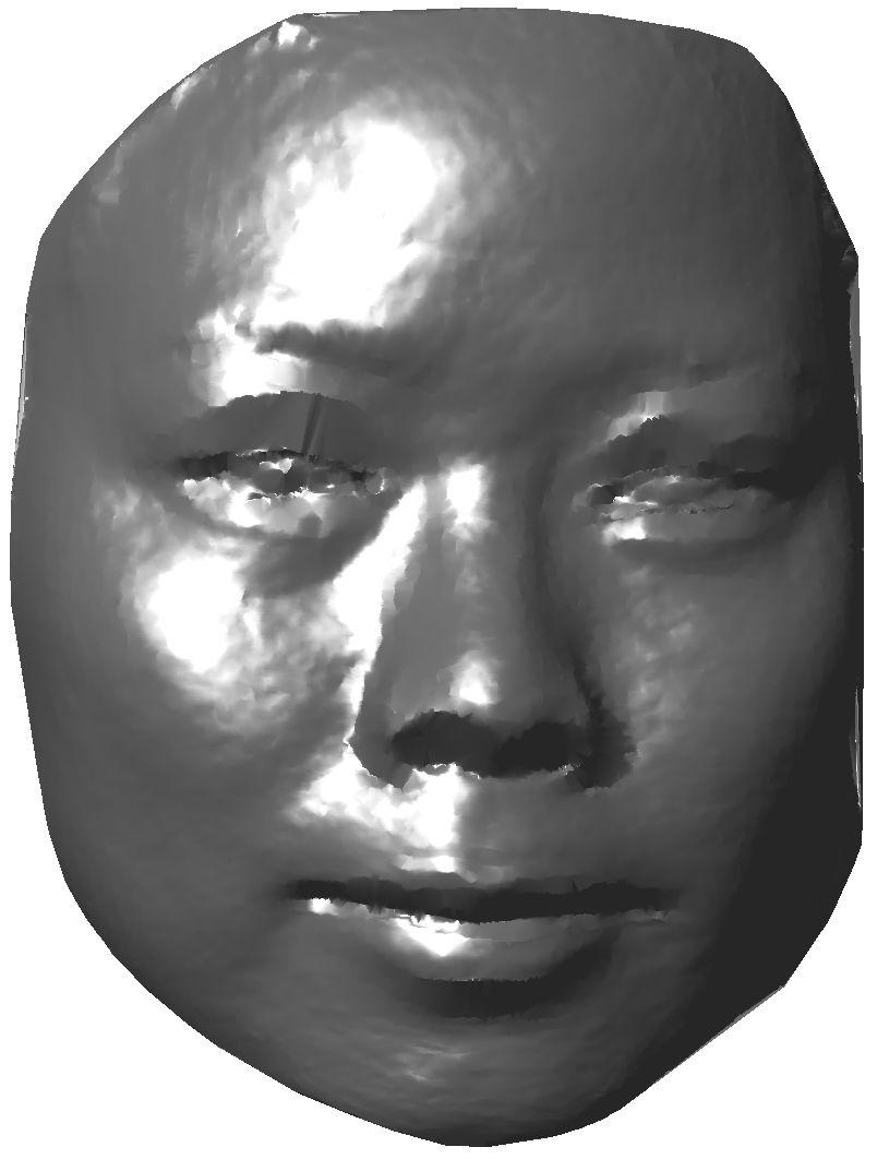
81 65 (a) (b) (c) (d) Figure 4.4

82 vertex pairs of the conformed generic model to construct a set of weak classifiers for face recognition The Fast Marching Method on Triangulated Domains The Fast Marching Method (FMM), proposed by Sethian in [83], is a technique for computing geodesic distances across a triangulated surface. The FMM is a method for tracking the evolution of an expanding front. It computes the arrival time of a front at the vertices of a discrete lattice. Given a surface, the FMM can be used to compute its distance field, since, if the front evolves at unit speed, the arrival time corresponds to the distance. The front expands in the direction of the surface normals. At a given point, the motion of the front is described by the Eikonal equation: T F(x,y) = 1 (4.6) where T and F(x,y) 0 are the arrival time and the speed of the front at point (x, y), respectively. The aim of the FMM is to expand the front from a starting vertex. Say we are computing the distance field from a vertex, p. In this case, p would be used as the starting vertex of the expanding front. The starting vertex is tagged as frozen, and distances are computed at its neighbors. Vertices that have computed distances but are not yet frozen are designated as narrow band vertices. For each iteration of the method, the narrow band vertex having the smallest distance value is frozen, and distances are computed at its neighbors. Frozen vertices are utilized to compute the distance values of other vertices but are never computed again. Thus, the method propagates a front of narrow band points from the starting vertex, freezing points as it traverses the surface.

83 Distances are computed by solving the Eikonal equation. The distance value foranarrowbandvertex isobtainedsuch thattheestimated lengthofthegradient, T, is equal to 1/F. 67 T = 1/F (4.7) Sethian proposes the following formula (taken from the field of hyperbolic conservation laws) for the squared length of the gradient: max(v 1 V 2,V 1 V 3,0) 2 + T 2 = max(v 1 V 4,V 1 V 5,0) 2 + (4.8) max(v 1 V 6,V 1 V 7,0) 2 where V 1 is the unknown distance value and {V i } 7 i=2 are the distance values at the neighboring vertices (in the six-connected neighborhood) illustrated in Figure 4.5(a). Equation (4.7) is then substituted into (4.8), which leads to the following equation: max(v 1 V 2,V 1 V 3,0) 2 + 1/F 2 = max(v 1 V 4,V 1 V 5,0) 2 + (4.9) max(v 1 V 6,V 1 V 7,0) 2 In (4.9), terms that do not contain a minimum of one frozen vertex are discarded from the equation. Assuming V 2 < V 3,V 5 < V 4,V 6 < V 7 and that V 2, V 5, and V 6 are frozen, the following quadratic equation is formed: (V 1 V 2 ) 2 +(V 1 V 5 ) 2 +(V 1 V 6 ) 2 = 1/F 2 (4.10) The largest solution to this equation is the one sought. This follows from the fact that V 1 must be greater than the three known values (since they are frozen). The interested reader is referred to [3] for a more detailed description of the method. Figure 4.5(b) illustrates several geodesic distances that have been computed for a sample 3D face model.

84 (a) (b) Figure Implementation In our experiments, we use the geodesic distances from a set of source vertices to a subset of their surrounding vertices as features. Since there is a one-to-one correspondence between the vertices of the conformed generic model instances, the same index map applies to all models. There is a total of 328 source vertices that are uniformly distributed across the facial region and are localized on the index map, as shown in Figure 4.6(a). The destination vertices for a given source vertex (shown in Figure 4.6(d)), p src = (x,y), are computed on the index map as p des = (x+rcosθ,y +rsinθ), where four distances, r {15,30,40,60}, and 24 orientations, θ { 0, 1, 2 23,, 2π 2π 2π}, are used. The projection of these points from the index map onto the 3D face models is illustrated in Figure 4.6(b,c,e,f). 4.5 Learning the Most Discriminant Geodesic Distances Between Anatomical Point Pairs by AdaBoost We construct a set of weak classifiers for face recognition using the geodesic distances described in the previous section. We use the Adaboost learning algorithm, formulated by Freund and Schapire [35], to train a strong classifier based on a

85 69 (a) (b) (c) (d) (e) (f) Figure 4.6

86 70 weighted selection of weak classifiers. The performances of three Adaboost algorithms, namely, the original Freund and Schapire method termed Real Adaboost, and two variants, Gentle Adaboost and Modest Adaboost, are investigated. The various AdaBoost algorithms presented here primarily differ in the update scheme of the weights. The following section will describe these Adaboost methods as well as the method of constructing the weak classifiers known as classification and regression trees Real Adaboost Boosting is a method of obtaining a highly accurate classifier by combining many weak classifiers, each of which is only moderately accurate. The following briefly describes the original Adaboost algorithm, proposed by Freund and Schapire [35], which we term Real Adaboost. Let S = {(x i,y i )} M i=1 be a sequence of M training examples where sample x i R N belongs to a domain or sample space χ, and each label y i belongs to a binary label space Υ = { 1,+1}. Each sample x i is comprised of a set of N features, such as the geodesic distances between a set of anatomical point pairings employed in this work. A weak classifier is used to generate a predicted classification for a sample based on the value of a single feature. The weak classifiers in this work are constructed using the Classification and Regression Trees (CART) method, which is described in Section The idea of boosting is to use a set of weak classifiers to form a highly accurate classifier by calling the weak classifiers repeatedly with different weighting distributions over the training examples. Boosting is comprised of three key steps: 1) computing the weight distribution, 2) training the weak classifier and 3) computing a real-valued function, f t. The AdaBoost algorithm runs for T iteration, where each sample x i is assigned a weight w t (i) at each iteration t = {1,...,T}. Initially, all weights are set equally, and are redistributed at each iteration in order to ma-

87 nipulate the selection process. At each iteration t, the weak classifier produces a mapping h t (x) : χ R, where the sign of h t (x) provides the classification, and h t (x) is a measure of the confidence in the prediction. The class predictions are then used to construct a weighted class probability estimate given by: p t (x) = ˆP w (y = +1 x) [0,1] (4.11) The weights are then redistributed and normalized as follows: 71 w t+1 (i) = w t(i)exp( y i h t (x i )) Z t (4.12) Increasing the weights of samples that are misclassified by h t, in the next iteration, favors the weak classifiers that handle correctly these difficult samples. Z t denotes the normalization factor which ensures that the sum of all weights equals 1. The contribution to the final classifier is the logit-transform of the class probability estimate given by: f t (x) = 1 ( ) 2 log pt (x) 1 p t (x) (4.13) A pseudocode outline of the Real Adaboost method is given in Algorithm 3. Algorithm 3 The Real Adaboost Algorithm 1: Given M training samples {(x i,y i )} M i=1,x i R N,y i { 1,+1} 2: Initialize weights w 1 (i) = 1/M 3: for t = 1,...,T do 4: Train the weak classifier, h t (x), and compute the class probability estimate, p t (x) = ˆP w (y = +1 x) ( [0,1],) using weight distribution w t 5: Compute f t (x) = 1 log pt(x) 2 1 p t(x) 6: Update w t+1 (i) = wt(i)exp( y ih t(x i )) Z t 7: end for ( T ) 8: Strong classifier: sign(f (x)) = sign t=1 f t(x) Gentle Adaboost The main difference between the Gentle Adaboost method (proposed by Friedman et al. in [36]) and the Real Adaboost method is how it uses its weighted class

88 72 probabilities, p t (x), to compute the real-valued function, f t (x). Here the equation is given as f t (x) = P w (y = +1 x) P w (y = 1 x), rather than half the log ratio as in (4.13). It has been shown that log ratios can be numerically unstable [36], leading to very large update values, while the update here lies in the range [ 1, +1]. Additionally, fitting of the weak classifier is performed using weighted least squares, given by: h t = argmin h ( M ) w t (i) (y i h(x i )) 2 i=1 (4.14) An outline of the Gentle Adaboost method is given in Algorithm 4. Algorithm 4 The Gentle Adaboost Algorithm 1: Given M training samples {(x i,y i )} M i=1,x i R N,y i { 1,+1} 2: Initialize weights w 1 (i) = 1/M 3: for t = 1,...,T do 4: Fit the weak classifier, h t (x), by weighted least squares of y i to x i and compute the class probability estimate, p t (x) = ˆP w (y = +1 x) [0,1] 5: Compute f t (x) = p t (x) (1 p t (x)) 6: Update w t+1 (i) = wt(i)exp( y if t(x i )) Z t 7: end for 8: Strong classifier: sign(f (x)) = sign ( T ) t=1 f t(x) Modest Adaboost The Modest Adaboost algorithm, proposed by Vezhnevets and Vezhnevets in [95], has shown in certain instances to generalize better than the previously mentioned methods, sometimes at the cost of higher training error. Another advantage of the method is a natural stopping criterion, which other boosting techniques lack. Similarly to the previous two methods, we compute the values p +1 t (x) = ˆP w (y = +1 h t (x)) and p 1 t (x) = ˆP w (y = 1 h t (x)), which are measurements of the classification accuracy of the current weak classifier, weighting higher samples that have been misclassified. In contrast, the additional values p +1 t (x) =

89 ˆP w (y = +1 h t (x)) and p 1 t (x) = ˆP w (y = 1 h t (x)) are measurements of the classification accuracy, weighting higher samples that have been correctly classified. The Modest Adaboost algorithm sets f t (x) = ( ( ) ( )) p +1 t 1 p +1 t p 1 t 1 p 1 t (x) in order to decrease the contribution of weak classifiers that perform too well in classifying data that has already been correctly classified with high margin; Thus, the name Modest Adaboost. An outline of the Modest Adaboost method is given in Algorithm 5. Algorithm 5 The Modest Adaboost Algorithm 1: Given M training samples {(x i,y i )} M i=1,x i R N,y i { 1,+1} 2: Initialize weights w 1 (i) = 1/M 3: for t = 1,...,T while h t 0 do 4: Fit the weak classifier, h t (x), by weighted least squares of y i to x i 5: Compute the inverted weight distribution w t (i) = (1 w t (i)) Z t 6: Compute the class probability estimate p +1 t (x) = ˆP w (y = +1 h t (x)) [0,1] p +1 t (x) = ˆP w (y = +1 h t (x)) [0,1] p 1 t (x) = ˆP w (y = 1 h t (x)) [0,1] p 1 t (x) = ˆP w (y = 1 h t (x)) [0,1] 7: Compute f t (x) = ( ( ) p +1 t 1 p +1 t p 1 t ( )) 1 p 1 t (x) 8: Update w t+1 (i) = wt(i)exp( y if t(x i )) Z t 9: end for ( T ) 10: Strong classifier: sign(f (x)) = sign t=1 f t(x) Classification and Regression Trees CART, proposed by Breiman et al. [11], is a decision tree learning method that is typically used to generate weak classifiers for the AdaBoost algorithm. The objective is toconstruct a model thatpredicts thevalue or class ofatarget variable based on one or more input variables. CART is a form of binary recursive partitioning. The term binary implies that each tree node, containing a decision rule, can only be split into two decisions.

90 74 Thus, each node can be split into two child nodes, in which case the original node is called a parent node. The term recursive refers to the fact that the binary partitioning process can be applied repeatedly. Thus, each parent node can give rise to two child nodes and, in turn, each of these child nodes may themselves be split, forming additional children. The term partitioning refers to the fact that the dataset is split into subsets or partitioned. At the end of each tree path is a leaf node that contains the predicted class label or value of its subset. The recursion process is completed when all variables contained in a node have the same value of the target variable, or when splitting no longer adds value to the predictions. In our algorithm, we select decision stumps as weak classifiers. A decision stump is a decision tree with a root node and two leaf nodes. For each feature in the input data, a decision stump is constructed. The following points support our selection of decision stumps as the weak classifiers: 1) the model that decision stumps use is very simple and 2) there is only one matching operation in each decision stump for testing a sample; thus, the computational complexity of each decision stump is very low Intra-Class and Inter-Class Space The Adaboost algorithm works with binary (two-class) classifiers, and face recognition is effectively a multi-class problem. Therefore, the face recognition problem must be transformed from a multi-class problem to a two-class problem. We employ a statistical approach to construct two classification spaces, namely, the intra-class space and the inter-class space [78]. The intra-class space, CI, is formed by analyzing the variations in geodesic distances between the conformed generic model instances of an individual. Conversely, the inter-class space, CE, is formed by analyzing the variations in geodesic distances between the conformed generic models of different individuals. Firstly, let the set of geodesic distances

91 75 extracted from a given conformed generic model, M, be denoted by G(M) = {D(p i,p j ) i [1,...,N src ],j [1,...,des(p i )]}whered(, )representsthegeodesic distance, N src is the number of source vertices, and des(p i ) denotes the number of destination vertices associated with source vertex p i. The intra-class and interclass spaces are respectively defined as: CI ={ G(M p ) G(M q ),{M p,m q } A i } (4.15) CE={ G(M p ) G(M q ),M p A i,m q A j } (4.16) where M p and M q are the conformed generic models taken from subject p and q, respectively. In the CI case, M p and M q are two model instances that belong to the same subject class A i. Conversely, in the CE case, M p and M q are two model instances that belong to different subject classes A i and A j, where C i=1a i = (C denotes the number of subject classes). Samples of class CI are designated with label +1 and samples of class CE with Implementation Given a training set that includes N images for each of K individuals, the total number of image pair combinations is C KN 2, where the majority of pairs belong to the CE class and a small minority of K C N 2 pairs belong to the CI class. In order to select a subset of samples to represent the overwhelmingly large number of CE samples, andtomanagetheimbalancebetweenci andce samples, weemploythe re-sampling scheme proposed in [105]. Algorithm 6 outlines the training process. The final classifier, F (x), is the summation of a set of strong classifiers, F q (x) = T t=1 f t(x), where each F q (x) is a collection of weak classifiers obtained from the q th iteration s training samples. After each iteration, a re-sampling scheme is employed to replace CE samples for the subsequent iteration. Because of the limited number of CI samples, all CI samples are retained in each iteration, and

92 Algorithm 6 Training process with re-sampling scheme 1: Giventhelabeledtrainingset X, include allci samples andselect CE samples randomly at the rate of 1:2 to generate a training subset x X. 2: for q = 1,...,Q do 3: Perform AdaBoost on x for t = {1,...,T q } iterations such that FAR 2%, FRR = 0%. This produces a collection of weak classifiers F q (x) = Tq t=1 f t(x) 4: Replace the CE samples of x; if sign(f q (x i )) y i, add it to the training subset, x. 5: end for ( Q ) 6: Final classifier: sign(f (x)) = sign q=1 F q(x) 76 only CE samples are re-sampled. If at iteration q, a CE sample, x i, is misclassified bythestrongclassifier, F q (x), x i isaddedtothesetoftrainingsamplesforiteration q+1. The number of Adaboost iterations, T, is contingent on the strong classifier, F q (x), achieving an acceptable false positive and false negative classification rate. Each iteration of the training process has a False Acceptance Rate (FAR) of 2% and a False Rejection Rate (FRR) of 0%, ensuring that the trained classifier is capable of separating the CI samples from the CE samples. The ratio of CI samples to CE samples is maintained at 1:2 due to the imbalance between CI and CE samples. 4.6 Experimental Setup We evaluated the proposed method on the FRGC v1.0 2D + 3D frontal face database D collection, which is comprised of 953 registered 2D + 3D images of 277 human subjects [19]. These images were acquired at the University of Notre Dame between January and May Two four-week sessions were conducted for data collection, approximately six weeks apart. Subjects participated in one or more acquisitions, with a minimum of one week between successive acquisitions. Among 277 subjects, 200 participated in more than one acquisition. The range

93 77 scans of 15 subjects are either misaligned with their corresponding 2D images or contain occlusions within the facial region and have been excluded from our experiments. In each acquisition session, subjects were imaged using a Minolta Vivid 900 range scanner. Subjects stood approximately 1.5 meters from the camera, against a homogeneous background, with one front-above-center spotlight illuminating their face. They were instructed to maintain a neutral facial expression and to look directlyat thecamera. TheMinoltaVivid 900uses aprojected light stripetoacquire triangulation-based range data. It also captures a color image near-simultaneously with the range data capture. The result is a sampling of range data and a registered color image. 4.7 Experimental Results For the following experiments, the database was split into a training set and a testing set. The range image of subjects possessing a single range image is automatically enrolled in the training set. Subjects who underwent more than one acquisition have two of their range images enrolled in the testing set and the remainder in the training set. Subjects possessing two range images have them both enrolled in the testing set. This resulted in a training set consisting of 525 range images of 233 subjects and a testing set of 370 range images of 185 subjects. The testing set was further subdivided into a probe and gallery set, enrolling one range image of each subject into each set. The training set yielded 627 and 136,923 intra-class and inter-class range image pairs, respectively. At any given training iteration, all 627 intra-class pairs and 1,254 inter-class pairs are used, resulting in a training subset consisting of 1,881 samples.

94 78 The method described in Section 4.4 resulted in 24, 158 geodesic distance features per conformed generic model instance. A training process was performed using each of the Adaboost algorithms described in Section 4.5. For each training process, the same initial conditions were given, such as identical initial training subsets as well as the same number of re-sampling iterations. Intermediary conditions, such as the samples selected in the re-sampling scheme, differed amongst the algorithms as these conditions are algorithm-specific. Each training process iterated through 8 stages, and generated a final classifier consisting of 471, 553, and 378 weak classifiers for the Real Adaboost, Gentle Adaboost, and Modest Adaboost algorithms, respectively. To evaluate the performance of the proposed method, we applied the final classifiers obtained from each of the Adaboost algorithms to the probe and gallery sets of the testing set. Intra-class and inter-class pairs were constructed between a probe image and all images contained within the gallery. This resulted in one intra-class pair and 184 inter-class pairs for each subject in the probe set. The Adaboost classifiers were then applied to the sample set of each subject to produce the class predictions. As mentioned in Section 4.5.1, the sign of the classifier output provides the classification, and the absolute value is a measure of the confidence in the prediction. Therefore, a match score can be derived based on the absolute value of the classifier output, and since intra-class pairs are labeled as positive, the maximum match score would be the rank-one result. Algorithm 7 outlines the recognition process. The CMC curve, which illustrates the probability of identification against the returned 1:N candidate list size, is provided in Figure 4.7. The faster the CMC curve approaches 1, indicating that the subject always appears in the candidate list of specified size, the better the matching algorithm. It can be seen from this

95 79 Algorithm 7 Recognition Process 1: gallery samples (x g i,yg i ),i = 1,2,...,M,xg i RN 2: probe samples (x p i,yp i ),i = 1,2,...,L,xp i RN 3: for u = 1,...,L do 4: for v = 1,...,M do 5: F v (x p u ) = t f t( x p u xg v ) 6: end for 7: yu p = yg i,i = argmaxf v (x p u ) v=1,...,m 8: end for figure that the Gentle Adaboost algorithm, achieving a rank-one recognition rate of 95.69%, outperforms both the Real Adaboost and Modest Adaboost algorithms, achieving rank-one recognition rates of 94.59% and 91.89%, respectively. 100 Cumulative Match Characteristic (CMC) Curve Recognition Rate (%) Gentle Adaboost Real Adaboost Modest Adaboost Rank Figure 4.7 To assess the verification performance of the Adaboost algorithms, the ROC curves have been generated and are provided in Figure 4.8. An ROC curve plots, parametrically as a function of the decision threshold, the rate of false positives (i.e., impostor attempts accepted) on the x-axis, against the corresponding rate of true positives(i.e., genuine attempts accepted) on the y-axis. The Gentle Adaboost

96 80 algorithm, achieving a correct verification rate of 86.49% at a False Acceptance Rate (FAR) of 0.01 and an EER of 4.31%, outperforms both the Real and Modest Adaboost algorithms, achieving correct verification rates of 83.24% and 83.24% at a FAR of 0.01 and EERs of 4.71% and 4.87%, respectively. 100 Receiver Operating Characteristic (ROC) Curve 90 Correct Verification Rate (%) Gentle Adaboost Real Adaboost Modest Adaboost FAR Figure 4.8 Table 4.1 Authors, reference Subjects Images Matching algorithm Rank-1 Rate Kakadiaris et al., [47] Deformable model 99.3% Russ et al., [79] Hausdorff distance 98.5% Lin et al., [54] Summation-invariant features Tang et al., [88] N/A N/A Profile curve EER: 5.5% Berretti et al., [6] SIFT 70% proposed approach Geodesic distance 95.7% Ver.: 0.1% FAR For the remainder of the experiments, we only report the results of the Adaboost algorithm that demonstrated the highest rank-one identification and verification performance the Gentle Adaboost algorithm. In Figure 4.9, a plot of the rank-one identification rate as a function of the number of weak classifiers

97 comprising the final classifier is provided. As shown, the rank-one recognition rate improves from 40.54% with 60 weak classifiers to 95.68% with 553 weak classifiers Recognition Performance 90 Rank one Recognition Rate (%) Number of Weak Classifiers Figure 4.9 The weighted distribution of geodesic distance endpoint features contributing to the weak classifiers selected by the Gentle Adaboost algorithm is illustrated in Figure Both the source and destination vertices of each contributing feature areaccountedforinconstructing anaccumulator ofsize (e.g., thedimensions of a range image). For instance, if the classifier contains a geodesic distance feature comprised of source vertex p src and destination vertex p des, the index positions of the accumulator corresponding to both p src and p des will be incremented by the weight associated with the feature. A Gaussian low-pass filter with a variance of 2.0 is subsequently applied to smoothen the accumulator. The colors of the map represent the weighted proportion of selected features associated with a vertex; dark blue and dark red indicating maximal and minimal contributions, respectively. This illustrates that the most discriminant facial regions are the areas

98 around the nose, eye brows, mouth, and chin (e.g., high curvature regions) when using geodesic distance features. 82 Figure 4.10 In Table 4.1, we compare our results with the most notable systems [79, 47] systems applied to this dataset. Although the rank-one recognition rate reported here is less than those reported in [79, 47], the advantage of our approach is in the computational efficiency of the matching process. As discussed in Section 4.5.4, there is only one matching operation in each decision stump for testing a sample; thus, the computational complexity for each decision stump is extremely low. The final classifier is a weighted collection of decision stumps. As there are n weak classifiers comprising the final classifier, the computational complexity of testing a sample is O(n). In the case of the Gentle Adaboost algorithm, which generated a strong classifier based on a collection of 553 weak classifiers, the matching process requires 553 steps. The computational complexity reported in [79] is O(N), where N is approximately equal to K 30,000 vertices and K 20 denotes the number of iterations used for fine-tuning the face model registration; this results in a time complexity of approximately 30, = 600,000 steps (the proposed matching process is 1, times faster). The matching process proposed in [47] consists of computing the L 1 -norm distances between 1-channel and 3-channel deformation

99 83 images of a probe and gallery subject. The computational complexity of this method is O(N), where N denotes the number of vertices in the facial region. In the case that N = 4 30,000 vertices, the computational complexity of this method is 120,000 steps (the proposed matching process is 217 times faster). The methods presented in [54, 88, 6] are also applied to the FRGC v1.0 dataset, however, the authors do not provide a computational complexity analysis. 4.8 Conclusion In this chapter, we have presented a method for 3D face recognition using adaboosted geodesic distance features. Experiments were conducted on the publiclyavailable FRGC v1.0 2D + 3D frontal face database D collection. The classification performances of three Adaboost algorithms namely, the Real, Gentle, and Modest Adaboost algorithms were assessed on a gallery and probe set each consisting of 185 subjects. Experimental results indicate that the Gentle Adaboost algorithm outperforms the Real and Modest Adaboost algorithms in both the identification and verification tasks. The Gentle Adaboost algorithm achieved an 95.68% rank-one recognition rate and an EER of 4.31% based on a classifier containing 553 geodesic distance features. The geodesic distances selected by the Gentle Adaboost algorithm are contained primarily within the regions of the nose, eye brows, mouth, and chin. These salient facial regions are consistent with those reported in psycho-visual analyses of human face perception and recognition [39]. Conventional shape matching methods commonly used in 3D face recognition are time consuming. Such is the case with the Iterative Closest Point ICP [7] method, which has a computational complexity of O(N 2 ), where N denotes the number of vertices comprising the 3D surfaces. The proposed approach can be applied as a data reduction technique to reduce the number of vertices consid-

100 84 ered when matching 3D facial data; effectively increasing computational efficiency (executes in linear time) while maintaining an acceptable recognition rate. In this work we directly used the geodesic distance between a source and destination vertex as a feature. We acknowledge that these features are not robust to surface noise, and do not incorporate information about the shape of the geodesic curve. Future work will include investigating the use of integral invariant signatures[33] to represent the geodesic paths. These features are more robust to surface noise and incorporate shape information about the geodesic paths. To extend the proposed method to faces demonstrating facial expressions, future work will also include generating a bending-invariant canonical representation of the facial surface, as proposed in [12], prior to performing the surface registration described in Section 4.3. This representation, obtained by Multi-Dimensional Scaling (MDS), is invariant to isometric transformation of the surface, which a variety of facial expressions has been shown to adhere to [12]. The transformation of the facial surface into a bending-invariant canonical representation effectively reduces the non-rigid registration of two surfaces demonstrating different expressions into a rigid registration problem, to which the proposed method can be applied.

101 Chapter Five A Computationally Efficient Approach to 3D Ear Recognition Employing Local and Holistic Features 5.1 Overview 3D object recognition is an attractive field of research because of its theoretical merits as well as its usability in a broad range of applications. A 3D object can be represented by a complimentary set of local and holistic features. Local features are robust to clutter and small amounts of noise. In contrast, holistic features are easier to construct and retain more information about an object than local features. The majority of 3D object recognition systems focus solely on one feature category [16]. However, the use of a single feature category may be insufficient when recognizing highly similar objects. It is therefore desirable in these scenarios to develop a system that incorporates local and holistic features in a scalable and efficient manner. In this chapter, we present a 3D object recognition system capable of discriminating between highly similar 3D objects. An evaluation of the proposed system is conducted on a 3D ear recognition task. The ear provides a challenging case study because of its high degree of inter-subject similarity. The system is comprised of four primary components: 1) object segmentation, 2) local feature extraction and matching, 3) holistic feature extraction and matching, and 4) a fusion framework combining local and holistic features at the match score level. For the segmentation component, we employ the method presented in [111]. For the local feature extraction and representation component, we extend the Histogram of Indexed 85

102 86 Shapes (HIS) feature descriptor, proposed in [111], to an object-centered 3D shape descriptor, termed SPHIS, for surface patch representation and matching. For the holistic feature extraction and matching component, we propose voxelizing the object surface to generate a representation from which an efficient, voxel-wise comparison of gallery-probe model pairs can be made. The match scores obtained from both the local and holistic matching components are fused to generate the final match scores. An overview of our system is provided in Figure 5.1. The remainder of this chapter is organized as follows: Sections 5.2 and 5.3 present the local and holistic feature extraction and matching components, respectively. Section 5.4 details the match score level fusion framework used. Section 5.5 provides the experimental results obtained from an identification and verification task. Lastly, conclusions and future research directions are discussed in Section Local Feature Representation Preprocessing Prior to extracting the local feature representation from a range image, a series of preprocessing steps is performed. Firstly, we apply the 3D ear detection system proposed in [111]. This system outputs a Bounding Box (BB) from which the ROI can be cropped and used as input for the feature extraction stage. Secondly, to reduce noise in the input image (e.g., spikes and holes), preprocessing is also necessary before performing the feature extraction. The data preprocessing in our implementation consists of three successive steps: 1) median

103 Figure

104 88 filtering to remove spikes, 2) cubic interpolation to fill the holes in the data, and 3) a Gaussian filter to smooth the data. Thirdly, the surface is normalized to a standard pose. The centroid of the surface is firstly mapped to the origin of the coordinate system. Then, the principal components corresponding to the two largest eigenvalues of the surface are calculated. The surface is then rotated such that the two principal components are aligned with the x and y axes of the coordinate system. The utility of the pose normalization becomes evident in Section Histogram of Indexed Shapes (HIS) Feature Descriptor Objects can be characterized by their distinct 3D surface shapes. The human ear, for instance, contains areas around the helix ring and anti-helix that possess both prominent saddle and ridge shapes, while the inner ear regions are comprised of rut and trough shapes Shape Index and Curvedness A quantitative measure of the shape of a surface at a point p, called the shape index S I, is defined as [30]: S I (p) = ( ) π arctan kmax (p)+k min (p) k max (p) k min (p) (5.1) where k max and k min are the principal curvatures of the surface at point p, with k max > k min defined as: k max (p) = H(p)+ H 2 (p) K(p) (5.2) k min (p) = H(p) H 2 (p) K(p) (5.3) where H(p) and K(p) are the mean and Gaussian curvatures, respectively. Note that with the definition of S I in equation (5.1), all shapes can be mapped on the interval S I = [0,1]. Every distinct surface shape corresponds to a unique

105 89 value of S I, except for the planar shape. Vertices on a planar surface have an indeterminate shape index, since k max = k min = 0. The shape index value captures the intuitive notion of the local shape of a surface. Nine well-known shape categories and their corresponding shape index values are shown in Table 5.1 [30]. Table 5.1 Shape category S I Shape category S I Spherical cup (0, 1/16) Spherical cap (15/16, 1) Trough (1/16, 3/16) Dome (13/16, 15/16) Rut (3/16, 5/16) Ridge (11/16, 13/16) Saddle Rut (5/16, 7/16) Saddle Ridge (9/16, 11/16) Saddle (7/16, 9/16) The shape index of a rigid object is not only independent of its position and orientation in space, but also independent of its scale. To encode the scale information, we utilize the curvedness, which is also known as the bending energy, to capture the scale differences [30]. Mathematically, the curvedness of a surface at a point p is defined as: C v (p) = k 2 max (p)+k 2 min (p) 2 (5.4) It measures the intensity of the surface curvature and describes how gently or strongly curved a surface is HIS Descriptor To build the histogram descriptor, firstly, the curvedness and shape index values are computed at each point contained within the surface region to be encoded. Each point contributes a weighted vote for a histogram bin based on its shape index value, with a strength that depends on its curvedness. The votes of all

106 90 points are then accumulated into the evenly spaced shape index bins forming the HIS descriptor. The HIS descriptor is normalized with respect to its total energy D Keypoint Detection To generate the set of local features, the input image is initially searched to identify potential keypoints that are both robust to the presence of image variations and highly distinctive, allowing for correct matching. The keypoint detection method proposed here is inspired by the 3D face matching approach proposed by Mian et al. in[60], but with significant enhancements tailored towards improved robustness and applicability to objects with salient curvature, such as the ear. In the method presented by Mian et al., the input point cloud of the range image is sampled at uniform intervals. By observing 3D ear images, we found that the majority of these salient points are located in surface regions containing large curvedness values. This signifies that sampling in regions containing large curvedness values will result in a higher probability of obtaining repeatable keypoints. Instead of uniformly sampling the range image to obtain the candidate keypoints, we propose using a local b b (b = 1mm in our case) window to locate the candidate keypoints; the center point of the window is marked as a candidate keypoint only if its curvedness value is higher than those of its neighbors in the window. The keypoint repeatability experiment presented at the end of this section will demonstrate that by enforcing the keypoints to have a locally maximum curvedness value, more repeatable keypoints can be found. Once a candidate keypoint has been located, a local surface patch surrounding the candidate keypoint is cropped from the ear image using a sphere centered at the candidate keypoint. The purpose of examining its nearby surface data is to further reject candidate keypoints that are less discriminative or less stable due to their location in noisy data or along the image boundary. If the cropped surface

107 91 data contains boundary points, the candidate keypoint is automatically rejected as being close to the image boundary. Otherwise, PCA is applied to the cropped surface data, and the eigenvalues and eigenvectors are computed to evaluate its discriminative potential. A candidate keypoint is kept only if the eigenvalues computed from its associated surface region satisfy the following criteria: 3 3 λ 3 / λ i > t 1 and λ 1 / λ i < t 2 (5.5) i=1 i=1 where λ 1 and λ 3 are the largest and smallest eigenvalues. The threshold t 1 ensures that the cropped region associated with a keypoint has a certain amount of depth variation. Similarly, the threshold t 2 ensures that the keypoint is not located in a noisy region or edge where the data variation is mostly carried by one principal direction. In our implementation, t 1 and t 2 are chosen as t 1 = 0.01 and t 2 = 0.8. Figure 5.2 provides an overview of the keypoint detection procedure. Firstly, a set of candidate keypoints are sampled on the surface based on their curvedness values as shown in Figure 5.2(b). Secondly, PCA is performed on these keypoints neighboring points to reject inadequately distinctive and noisy candidate keypoints. Figure 5.2(c) demonstrates this PCA step, where the example candidate keypoints 1 (a less distinctive point), 2 (a noisy point) and3(a boundary point) are rejected, and the retained keypoints are shown in Figure 5.2(d). To demonstrate the effectiveness of our keypoint detection algorithm, a repeatability experiment is performed on the keypoints extracted from 200 3D ear images of 100 individuals in which each subject has a pair of ear images. Since the range images contain real data, the ground truth correspondences of the keypoints are unknown. In this experiment, an approximation of the ground truth correspondences is obtained using an ICP-based registration algorithm as suggested in [60]. The pair of ear models from the same subject is firstly registered using all

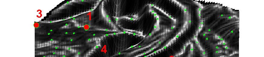
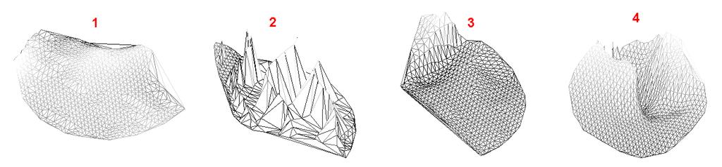
108 92 (a) (b) (c) (d) Figure 5.2

109 93 of the points comprising the models. A keypoint s nearest neighboring keypoint in the counterpart image is considered as its correspondence after the alignment. When the correspondence is located within a distance of the keypoint, it is considered as a repeatable keypoint. Figure 5.3 illustrates the cumulative repeatability percentage as a function of the increasing distance of the correspondences, where the line represents the mean performance across the dataset and the bars indicate a 90% confidence range. The repeatability reaches 28.6% at 1mm by sampling points with locally maximum curvedness values, compared to 20.1% obtained by a uniform sampling method. Notice that we only consider the repeatability at distances within the resolution of the data. Overall, our keypoint detection algorithm achieves a higher repeatability by sampling points possessing larger curvedness values. 60 Repeatability of Keypoints 50 Repeatability (%) % at 1 mm 20.7% at 1 mm 10 Local maxium curvedness points Uniform sampling Closest Point Error (mm) Figure 5.3

110 Local Feature Representation The locations of the detected keypoints provide repeatable local 3D coordinate systems to describe the local ear surfaces. The next step is to construct a feature descriptor to represent the local ear surface that is highly distinctive while remaining invariant to other changes, such as pose, background clutter and noise. Our local feature representation described below is an extension of the Histogram of Indexed Shapes (HIS) feature introduced in Section The extension includes a different computational mechanism that renders the feature representation more accurate and informative, allowing for the capture of more subtle inter-ear shape variations among different subjects Surface Patch Histogram of Indexed Shape (SPHIS) Descriptor As mentioned in Section 5.2.4, the HIS descriptor can be used to encode shape information of any surface region. In addition, we can form a HIS of arbitrary size by uniformly spacing the shape index values over the range [0,1]. The larger the dimensionality of the HIS, the more descriptive it is. However, too large of a descriptor may be sensitive to noise. Based on the HIS descriptor, the SPHIS descriptor is employed to represent the keypoint, and is built from the surface patch surrounding it. Figure 5.4 illustrates the procedure for constructing the SPHIS feature descriptor. Firstly, the surface patch surrounding a keypoint is cropped using a sphere cut that is centered on the keypoint with a radius r. The value of r determines the locality of the surface patch representation and offers a trade off between its distinctiveness and robustness. The smaller the value is, the less distinctive the surface patch while more resistant to pose variation and background clutter. Thus, the choice of r is dependent on the applied object. In

111 our 3D ear recognition implementation, the radius is set to r = 14mm, which is empirically determined based on the size of the human ear. 95 Figure 5.4 Secondly, the points contained within the cropped surface patch are further divided into four subsets using three additional concentric sphere cuts with radii of r i = i r,i = 1,2,3, which are all centered on the keypoint, forming four sub- 4 surface patches as shown in the second and third rows of Fig 5.4. The motivation behind dividing the cropped surface patch into sub-surface patches is to derive spatial information of the surface patch. After forming the four adjacent sub-surface patches, a HIS descriptor is built from each of the four sub-surface patches by voting their points curvedness values into the shape index bins as described in Section The SPHIS descriptor construction generates an array of 1 4 HIS descriptors with 16 bins (16 indexed shapes) from the four sub-surface patches, where the length of each bin corresponds to the magnitude of that histogram entry. This histogram is shown in the forth row of Figure 5.4. The four HIS descriptors are then concatenated to form a

112 96 64-dimensional feature vector. Lastly, the shape index value of the keypoint is appended to the feature vector to increase its discriminative potential and reduce the probability that keypoints exhibiting different shape types are matched in the feature matching stage. This results in a = 65 dimensional feature vector used to represent a local surface patch Local Surface Matching Engine In our local feature representation, a 3D ear surface is described by a sparse set of keypoints, and associated with each keypoint is a descriptive SPHIS feature descriptor that encodes the local surface information in an object-centered coordinate system. The objective of the local feature matching engine is to match these individual keypoints in order to match the entire surface. To allow for efficient matching between gallery and probe models, all gallery images are first processed. The extracted keypoints and their respective SPHIS feature descriptors are stored in the gallery. Each feature represents the local surface information in a manner that is invariant to surface transformation. A typical 3D ear image will produce approximately 100 overlapping features at a wide range of positions that form a redundant representation of the original surface. In the local feature matching stage, given a probe image, a set of keypoints and their respective SPHIS descriptors are extracted using the same parameters as those used in the feature extraction of the gallery images. For every feature in the probe image, its closest feature in the gallery image is determined based on the L 2 distance between the feature descriptors. A threshold t (t = 0.1 in our implementation) is then applied to discard the probe features that do not have an adequate match. This procedure is repeated for every probe keypoint, resulting in a set of initial keypoint correspondences. Outlier correspondences are then filtered using geometrical constraints. We apply the iterative orthogonal Procrustes

113 analysis method, described in Algorithm 8, to align the two sets of keypoints and eliminate outlier correspondences by assessing their geometric consistency. After applying this method, the local surface matching engine outputs the number of matched keypoints M for every probe-gallery pair as the similarity score. Figure 5.5 illustrates an example of recovering the keypoint correspondences from a pair of gallery and probe ear models. Algorithm 8 Iterative orthogonal Procrustes analysis for removing outliers 1: Given a set of M initial keypoint correspondences. Let gallery points g i = (x g i,yg i,zg i )T and probe points p i = (x p i,yp i,zp i )T, where i = 1,2,...,M 2: repeat 3: Align the keypoints of the gallery and probe models Calculate the centroids of the probe and gallery keypoints: g c = 1 M M i g i,p c = 1 M M i p i Find the rotation matrix R using singular value decomposition: C = 1 M i (p i p c )(g i g c ) T, C = UΛV T, R = VU T M Derive the translation vector t = g c Rp c Align the keypoints of the gallery and probe models using R,t: p i = Rp i +t Update the keypoint distances: d i = g i p i 2 4: Find the largest value in d i. If d max > 1.5mm, then the correspondence is removed and set to M M 1. 5: until d max < 1.5mm or M < 3 6: Output M as the similarity match score Holistic Feature Extraction Preprocessing The preceding section described the method by which to establish correspondences between a probe-gallery pair. The probe model is then registered onto the gallery model by applying the transformation obtained in the local matching stage to each point on the probe model. In the event that the number of established correspondences is below three, we rely on the pose normalization scheme, described in Section 5.2.1, for the model registration.

114 98 (a) (b) Figure 5.5

115 Surface Voxelization The holistic representation employed in this work is a voxelization of the surface. The motivation behind using such a feature is to explore alternative methods that are more efficient than computing the Mean Squared Error (MSE) between the registered probe and gallery models. Although employing the MSE measure to calculate surface similarity is often encountered in the literature [23, 104], it is a computationally expensive technique because it requires obtaining the nearest neighboring points of a surface on its counterpart(the complexity of a linear nearest neighbor search is O(N g N p ), where N g and N p denote the number of points comprising the gallery and probe models, respectively). A voxelization is defined as a process of approximating a continuous surface in a 3D discrete domain [96]. It is represented by a structured array of volume elements (voxels) in a 3D space. A voxel is analogous to a pixel, which represents 2D image data in a bitmap. Advantages of such a representation include a robustness to surface noise, which may occur when there is specularity on the surface upon acquisition. Its robustness to noise is enabled by the flexibility to vary the quantization step (i.e., the size of the voxel) used to discretize the surface. Furthermore, a voxelization may provide a condensed representation of the surface (depending on the size of the voxel used), which reduces the storage requirements of the database. Thirdly, voxelization methods are capable of producing normalized, fixed-sized representations across a set of varying objects. This enables efficient voxel-wise comparisons between representations (e.g., computing the dot product between them). Fourthly, it can encode attributes of a surface such as presence (i.e., whether a point on the surface is contained within a voxel), density (i.e., the number of points contained within a voxel), and surface characteristics (e.g., the mean curvedness of points contained within a voxel).

116 In this work, we propose to encode presence (a binary representation) to define the surface voxelization and investigate its efficacy Binary Voxelization The representation employed in this work is known as the binary voxelization. This representation simply encodes the presence of a vertex within a voxel. A voxel that has a point enclosed within it is assigned a value of 1 and 0, otherwise. Algorithm 9 describes the voxelization process using this feature. The inputs of this 100 algorithm are the points of the surface to be voxelized, {p i } N i=1, the voxel dimensions, {r x,r y,r z }, and the spatial extent of the voxel grid, {x lo,y lo,z lo,x hi,y hi,z hi }. The variable ɛ is used to ensure that points along the boundary of the voxel grid are assigned to voxels. Its value should be greater than zero but less than the minimum voxel dimension size (in our experiments, ɛ = ). A sample ear Algorithm 9 Binary Voxelization 1: Given surface vertices {p i } N i=1 = {x i,y i,z i } N i=1, voxel dimensions {r x,r y,r z }, and spatial extents {x lo,y lo,z lo,x hi,y hi,z hi } 2: Initialize: V = [v i,j,k ] sx s y s z = 0, where: 3: for i = 1,...,N do 4: v ψx(xi ),ψ y(y i ),,ψ = 1, where: z(z i ) 5: end for s x = (x hi +ɛ x lo )/r x s y = (y hi +ɛ y lo )/r y s z = (z hi +ɛ z lo )/r z ψ x (x i ) = (x i x lo )/r x +1 ψ y (y i ) = (y i y lo )/r y +1 ψ z (z i ) = (z i z lo )/r z +1 model before and after undergoing binary voxelization is illustrated in Figure 5.6.

117 101 (a) (b) (c) (d) Figure 5.6