Multiple View Geometry in Computer Vision
|
|
|
- Jemimah Floyd
- 5 years ago
- Views:
Transcription


1 Multiple View Geometry in Computer Vision

2 2
3 3
4 4
5 5

6 Visual 3D Modeling from Images 6


7 AutoStitch 7

8 Image Composite Editor redmond/groups/ivm/ice/ 8

9 Deep Zoom & HD View 9

10 Photosynth 10

11 PhotoCity 11
12 Projective Transformations
13 Homogeneous coordinates Homogeneous representation of lines ax by c 0 a,b,c T ka a,b,c T ~ ka,b,c T ( ) x ( kb) y kc 0, k 0 equivalence class of vectors, any vector is representative Set of all equivalence classes in R 3 (0,0,0) T forms P 2 Homogeneous representation of points x xy,,1 on l a,b,c T if and only if ax by c 0 T x,y, 1 a,b,c x,y, 1 l 0 T T x, y,1 ~ kx, y,1, k 0 The point x lies on the line l if and only if x T l=l T x=0 Homogeneous coordinates x, y, z T Inhomogeneous coordinates x, y T but only 2DOF 13
14 Points from lines and vice-versa Intersections of lines The intersection of two lines l and l' is x l l' Line joining two points The line through two points x and x' is l x x' Example y 1 x 1 14
15 Ideal points and the line at infinity Intersections of parallel lines l a, b, c T and l' a, b, c' T l l' b, a,0 T Example b, a a,b tangent vector normal direction x 1 x 2 Ideal points x, 2,0 T 1 x 0,0,1 Line at infinity T l P 2 R 2 l Note that in P 2 there is no distinction between ideal points and others 15
16 A model for the projective plane exactly one line through two points exactly one point at intersection of two lines 16
17 Duality x l x T l 0 l T x 0 x l l' l x x' Duality principle: To any theorem of 2-dimensional projective geometry there corresponds a dual theorem, which may be derived by interchanging the role of points and lines in the original theorem 17
18 Projective 2D Geometry 18
19 Projective transformations Definition: A projectivity is an invertible mapping h from P 2 to itself such that three points x 1,x 2,x 3 lie on the same line if and only if h(x 1 ),h(x 2 ),h(x 3 ) do. Theorem: A mapping h:p 2 P 2 is a projectivity if and only if there exist a non-singular 3x3 matrix H such that for any point in P 2 reprented by a vector x it is true that h(x)=hx Definition: Projective transformation x' x' x' h h h h h h h h h x x x or x' H x 8DOF projectivity=collineation=projective transformation=homography 19
20 Mapping between planes central projection may be expressed by x =Hx (application of theorem) 20
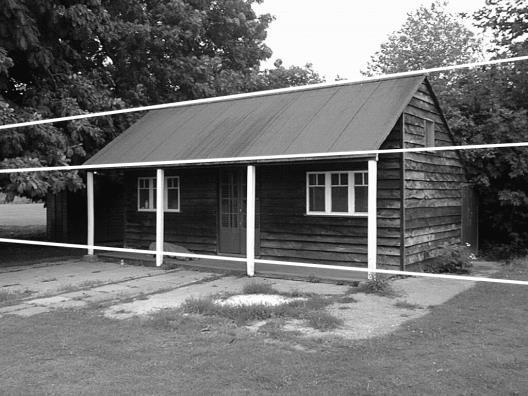
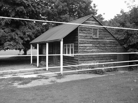
21 Removing projective distortion select four points in a plane with know coordinates x' 1 h11x h12y h13 x' 2 h21x h22y h x' y' x' h x h y h x' h x h y h x' y' h31x h32y h33 h11x h12y h13 h31x h32y h33 h21x h22y h (linear in h ij ) (2 constraints/point, 8DOF 4 points needed)

22 22
23 More Examples 23
24 Transformation for lines For a point transformation x' H x Transformation for lines l' H -T l 24
25 Isometries x' y' 1 cos sin 0 sin cos 0 tx x t y y orientation preserving: orientation reversing: 1 1 x' H E x R T 0 t x 1 R T R I 3DOF (1 rotation, 2 translation) special cases: pure rotation, pure translation Invariants: length, angle, area 25
26 Similarities cos sin sin cos 1 ' ' y x t s s t s s y x y x x 0 x x' 1 t T R H s S I R R T also know as equi-form (shape preserving) metric structure = structure up to similarity (in literature) 4DOF (1 scale, 1 rotation, 2 translation) Invariants: ratios of length, angle, ratios of areas, parallel lines
27 Affine transformations ' ' y x t a a t a a y x y x x 0 x x' 1 t T A H A non-isotropic scaling! (2DOF: scale ratio and orientation) 6DOF (2 scale, 2 rotation, 2 translation) Invariants: parallel lines, ratios of parallel lengths, ratios of areas DR R R A D
28 Projective transformations 28 x v x x' v P T t A H Action non-homogeneous over the plane 8DOF (2 scale, 2 rotation, 2 translation, 2 line at infinity) Invariants: cross-ratio of four points on a line (ratio of ratio) T 2 1, v v v v v s P A S T T T T v t v t A I K R H H H H T RK tv A s K 1 det K upper-triangular, decomposition unique (if chosen s>0)
29 Overview Transformations Projective 8dof Affine 6dof Similarity 4dof Euclidean 3dof h h h a a 0 sr sr 0 r11 r h h h a a r r sr sr h13 h 23 h 33 tx t y 1 tx t y 1 tx t y 1 Concurrency, collinearity, order of contact (intersection, tangency, inflection, etc.), cross ratio Parallellism, ratio of areas, ratio of lengths on parallel lines (e.g midpoints), linear combinations of vectors (centroids). The line at infinity l Ratios of lengths, angles. The circular points I,J lengths, areas. 29
30 Line at infinity v x v x v x x x x v A A T t x x x x v A A T t Line at infinity becomes finite, allows to observe vanishing points, horizon, Line at infinity stays at infinity
31 The line at infinity 31 v 1 v 2 l 1 l 2 l 4 l 3 l v 1 v 2 l l l v l l v The line at infinity l is a fixed line under a projective transformation H if and only if H is an affinity l t 0 l l A A H T T A
32 Affine properties from images projection rectification H PA 1 0 l1 0 1 l H l 3 A T l l l, l 0 l


33 Affine Rectification v 1 v 2 l l 1 l 3 l 2 l 4 v v l l1 2 l3 4 v 1 v 2 1 l 2 l 33


34 Projective 3D geometry Projective 15dof A T v t v Intersection and tangency Affine 12dof A T 0 t 1 Parallellism of planes, Volume ratios, centroids, The plane at infinity π Similarity 7dof s R T 0 t 1 The absolute conic Ω Euclidean 6dof R 0 T t 1 Volume 34
35 Camera Calibration
36 Pinhole Camera Model 36 T T Z fy Z fx Z Y X ) /, / ( ),, ( Z Y X f f Z fy fx Z Y X Z Y X f f Z fy fx
37 Pinhole Camera Model x K I 0X cam K f f px p y 1 Principal point offset Calibration Matrix 37
38 Internal Camera Parameters 38
39 Camera rotation and translation X ~ R X~ -C ~ cam RC ~ X R Y X cam 0 1 Z 1 R 0 RC X 1 x K I 0X cam x KR I C ~ X x PX P K R t t RC ~ 39
40 Camera Parameter Matrix P 40


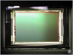

41 CCD Cameras 41

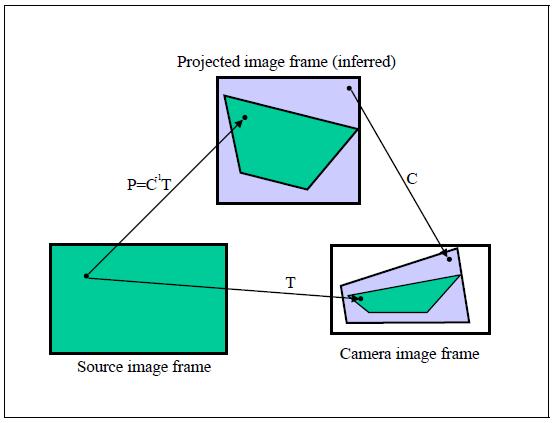
42 Correcting Radial Distortion of Cameras 42

43 43

44 Calibration Process 44
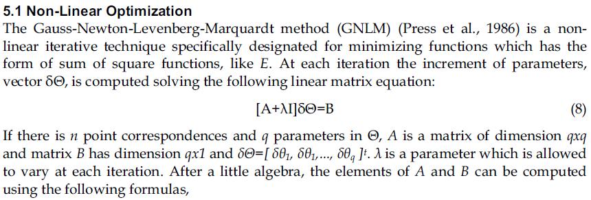
(1 k r k")
(1 k r k r k r )sin 2 4 6 u y")
cos 2 4 6 d y 1 d 2 d 3 d x y p p")

45 x c ( x c )(1 k r k r k r )cos u x d x 1 d 2 d 3 d ( y c )(1 k r k r k r )sin d y 1 d 2 d 3 d y c ( x c )(1 k r k r k r )sin u y d x 1 d 2 d 3 d ( y c )(1 k r k r k r )cos d y 1 d 2 d 3 d x y p p m x m y m m x 0 u 1 u 2 6 u m7yu 1 m x m y m m x 3 u 4 u 5 6 u m7yu 1 45


46 OpenCV alibration_and_3d_reconstruction.html 46

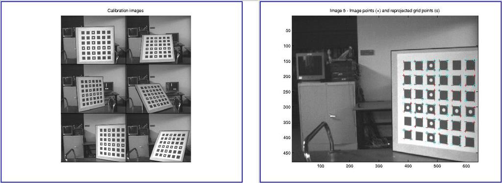
47 Camera Calibration Toolbox 47
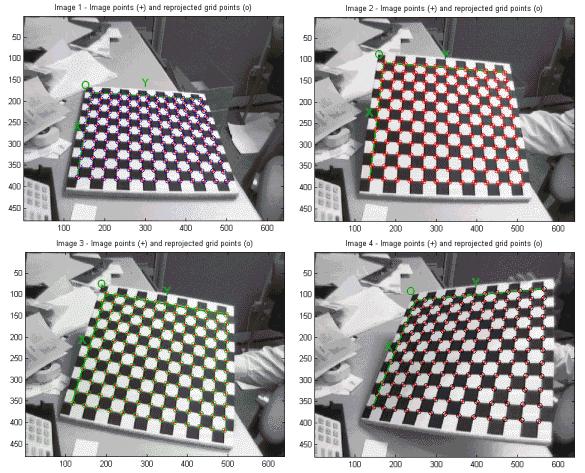
48 Camera Calibration 48
49 Calibrating a Stereo System 49

50 Robust Multi-camera Calibration 50

51 Multi-Camera Self Calibration 51
52 Multi-Camera Self Calibration 52
53 ARToolKit Camera Calibration 53
54 Epipolar Geometry and 3D Reconstruction.
55 Introduction Computer vision is concerned with the theory behind artificial systems that extract information from images. The image data can take many forms, such as video sequences, views from multiple cameras. Computer vision is, in some ways, the inverse of computer graphics. While computer graphics produces image data from 3D models, computer vision often produces 3D models from image data. Today one of the major problems in Computer vision is correspondence search. 55

56 Epipolar Geometry C,C,x,x and X are coplanar 56

57 Epipolar Geometry epipole 57
58 Epipolar Geometry All points on p project on l and l 58

59 Epipolar Geometry Family of planes p and lines l and l Intersection in e and e 59
 an epipolar line = intersection of epipolar plane with image (always come in corresponding")
60 Epipolar Geometry epipoles e,e = intersection of baseline with image plane = projection of projection center in other image = vanishing point of camera motion direction an epipolar plane = plane containing baseline (1-D family) an epipolar line = intersection of epipolar plane with image (always come in corresponding pairs) 60
61 The Fundamental Matrix F x' H π x l' e' x' e' H x Fx π H : projectivity=collineation=projective transformation=homography 61
62 Cross Products 62


63 Epipolar Lines 63
64 Three Questions (i) Correspondence geometry: Given an image point x in the first view, how does this constrain the position of the corresponding point x in the second image? (ii) Camera geometry (motion): Given a set of corresponding image points {x i x i }, i=1,,n, what are the cameras P and P for the two views? (iii) Scene geometry (structure): Given corresponding image points x i x i and cameras P, P, what is the position of (their pre-image) X in space? 64
65 Parameter estimation 2D homography Given a set of (x i,x i ), compute H (x i =Hx i ) 3D to 2D camera projection Given a set of (X i,x i ), compute P (x i =PX i ) Fundamental matrix Given a set of (x i,x i ), compute F (x i T Fx i =0) 65
66 The fundamental matrix F Algebraic Derivation X λ F e' P P' P x λc l' e' x' e' H x Fx l' P'C P'P x π P x P P I X λ (note: doesn t work for C=C F=0) 66
67 The fundamental matrix F Correspondence Condition The fundamental matrix satisfies the condition that for any pair of corresponding points x x in the two images x' T Fx 0 67


68 The Fundamental Matrix Song 68

69 The Fundamental Matrix 69
70 Epipolar geometry: basic equation 70 0 Fx x' T separate known from unknown 0 ' ' ' ' ' ' f yf xf f y yf y xf y f x yf x xf x 0,,,,,,,,,1, ',, ', ' ',, ', ' T f f f f f f f f f y x y y y x y x y x x x (data) (unknowns) Af 0 0 f 1 ' ' ' ' ' ' 1 ' ' ' ' ' ' n n n n n n n n n n n n y x y y y x y x y x x x y x y y y x y x y x x x
71 the NOT normalized 8-point algorithm f f f f f f f f f y x y y y y x x x y x x y x y y y y x x x y x x y x y y y y x x x y x x n n n n n n n n n n n n ~10000 ~10000 ~10000 ~10000 ~100 ~100 1 ~100 ~100! Orders of magnitude difference Between column of data matrix least-squares yields poor results
72 the normalized 8-point algorithm Transform image to ~[-1,1]x[-1,1] (0,500) (700,500) (-1,1) (0,0) (1,1) (0,0) (700,0) (-1,-1) (1,-1) Least squares yields good results (Hartley, PAMI 97) 72
73 The fundamental matrix F F is the unique 3x3 rank 2 matrix that satisfies x T Fx=0 for all x x (i) Transpose: if F is fundamental matrix for (P,P ), then F T is fundamental matrix for (P,P) (ii) Epipolar lines: l =Fx & l=f T x (iii) Epipoles: on all epipolar lines, thus e T Fx=0, x e T F=0, similarly Fe=0 (iv) F has 7 d.o.f., i.e. 3x3-1(homogeneous)-1(rank2) (v) F is a correlation, projective mapping from a point x to a line l =Fx (not a proper correlation, i.e. not invertible) 73
74 Fundamental matrix for pure translation 74


75 Fundamental matrix for pure translation 75
76 Fundamental matrix for pure translation e' e' F H 1 H K RK Example: 0 e' 1,0,0 T F 0 0 x' T Fx 0 y y' x x' PX K[I 0]X -1 P'X K[I t] K x Z ( X,Y,Z ) T -1 K x/z x' x Kt/Z motion starts at x and moves towards e, faster depending on Z pure translation: F only 2 d.o.f., x T [e] x x=0 auto-epipolar 76

77 General Motion x' x' T T x' e' Hx 0 e' xˆ 0 K'RK -1 x K't/Z 77
78 Projective transformation and invariance Derivation based purely on projective concepts xˆ x Hx, xˆ' H'x' Fˆ PX H' -1 PH H X Pˆ Xˆ -1 P'H H X Pˆ' Xˆ -T FH -1 F invariant to transformations of projective 3-space x' P'X P, P' F F P,P' unique not unique Canonical form P [I 0] P' [M m] F m M F e' P' P 78
79 Projective ambiguity of cameras given F 79 previous slide: at least projective ambiguity this slide: not more! Show that if F is same for (P,P ) and ~ (P,P ), ~ there exists a projective transformation H so that P=HP and P =HP P [I 0] P' [A a] F a A ~ a lemma: ~ a A ~ ka A ~ k 1 A av ~ ~ P [I 0] P' [A ~ ~ a] T af a a A 0 ~ af rank 2 T a A ~ a a ka ~ - A 0 ka ~ - A av A ~ 1 H k I 0 1 T k v k 1 P'H [A a] k I 1 k v T 0 k [ k ~ ~ 1 ~ T A -av ka] P' ~ a ka (22-15=7, ok)
80 Canonical cameras given F F matrix corresponds to P,P iff P T FP is skew-symmetric X T P' T FPX 0, X F matrix, S skew-symmetric matrix P [I 0] [SF e' ] T Possible choice: P [I 0] P' [SF e' ] T T F[I 0] F S F T e' F P' [[e'] F (fund.matrix=f) e' ] T 0 F S 0 0 T F 0 0 Canonical representation: P [I 0] P' [[e'] F e' v T λe'] 80
81 The Essential matrix ~ Fundamental matrix for calibrated cameras (remove K) t T E R R[R t] xˆ ' T E Exˆ K' T 0 FK xˆ 5 d.o.f. (3 for R; 2 for t up to scale) K -1 x; xˆ' K -1 x' E is essential matrix if and only if two singularvalues are equal (and third=0) T E Udiag(1,1,0)V 81
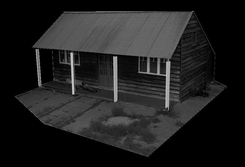


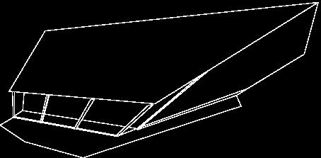
82 3D Reconstruction 82
83 Epipolar Geometry Underlying structure in set of matches for rigid scenes l T 1 l 2 T m F m1 2 0 Fundamental matrix (3x3 rank 2 matrix) C1 m1 l m1 1 e 1 e 2 P m2 l2 m2 C 2 M L2 L1 Canonical representation: P [I 0] P' [[e'] F e' v T λe'] 1. Computable from corresponding points 2. Simplifies matching 3. Allows to detect wrong matches 4. Related to calibration 83
84 3D reconstruction of cameras and structure Reconstruction Problem: given x i x i, compute P,P and X i xi PX i x i PX i for all i without additional informastion possible up to projective ambiguity 84
85 Outline of 3D Reconstruction (i) (ii) (iii) Compute F from correspondences Compute camera matrices P,P from F Compute 3D point for each pair of corresponding points computation of F use x i Fx i =0 equations, linear in coeff. F 8 points (linear), 7 points (non-linear), 8+ (least-squares) computation of camera matrices T use P [I 0] P' [[e'] F e' v λe' ] triangulation compute intersection of two backprojected rays 85
86 Reconstruction ambiguity: similarity x i PX i -1 PH H X S S i PH -1 S K[R t] R' 0 T - R' λ T t' K[RR' T RR' T t' λt] 86

87 Reconstruction ambiguity: projective x i PX i -1 PH H X P P i 87
88 Terminology x i x i Original scene X i Projective, affine, similarity reconstruction = reconstruction that is identical to original up to projective, affine, similarity transformation Literature: Metric and Euclidean reconstruction = similarity reconstruction 88
89 The projective reconstruction theorem If a set of point correspondences in two views determine the fundamental matrix uniquely, then the scene and cameras may be reconstructed from these correspondences alone, and any two such reconstructions from these correspondences are projectively equivalent x i x i P P P H P,P ', P,P ', 1 1 X1i P theorem from last class 2 2 X2i X except :Fx xf P 1H 2 HX1-1 HX1 i P1 H HX1 i P1 X1 i xi P2 2i 2 X along same ray of P 2, idem for P 2 two possibilities: X 2i =HX 1i, or points along baseline key result : allows reconstruction from pair of uncalibrated images i i 89

90 90
91 Stratified reconstruction (i) (ii) (iii) Projective reconstruction Affine reconstruction Metric reconstruction 91
92 Projective to affine Remember 2-D case 92
93 Projective to affine P,P', π T H - A, B, C, D T 0,0,0, 1 T X i π I 0 H π 0,0,0,1 T (if D 0) theorem says up to projective transformation, but projective with fixed p is affine transformation can be sufficient depending on application, e.g. mid-point, centroid, parallellism 93
94 Translational motion points at infinity are fixed for a pure translation reconstruction of x i x i is on p F [e] [e' ] P [I 0] P [I e'] 94
95 Scene constraints Parallel lines parallel lines intersect at infinity reconstruction of corresponding vanishing point yields point on plane at infinity 3 sets of parallel lines allow to uniquely determine p remark: in presence of noise determining the intersection of parallel lines is a delicate problem remark: obtaining vanishing point in one image can be sufficient 95
96 Scene constraints 96
97 Scene constraints Distance ratios on a line known distance ratio along a line allow to determine point at infinity (same as 2D case) 97
98 The infinity homography P [M m] P' [M' m' ] -1 H M' M unchanged under affine transformations P [M m] A a 0 1 H M' AA -1 M -1 [MA Ma m] X X ~,0 T affine reconstruction P [I 0] P [H e] x MX ~ x' M' X ~ 98
99 One of the cameras is affine According to the definition, the principal plane of an affine camera is at infinity to obtain affine recontruction, compute H that maps third row of P to (0,0,0,1) T and apply to cameras and reconstruction e.g. if P=[I 0], swap 3 rd and 4 th row, i.e. H


100 Affine to metric identify absolute conic transform so that : X Y Z 0, on π then projective transformation relating original and reconstruction is a similarity transformation 2 in practice, find image of W image w back-projects to cone that intersects p in W 2 2 * note that image is independent of particular reconstruction * 100
101 Affine to metric given P [M m] ω possible transformation from affine to metric is H A AA T T M ωm 1 (cholesky factorisation) proof: P ω M * M -1 ω PH M -1 M M -1 M -T [MA m] T M AA MAA T T M T * I
102 Orthogonality vanishing points corresponding to orthogonal directions T v ωv2 1 0 vanishing line and vanishing point corresponding to plane and normal direction l ωv 102
103 Correspondence and RANSAC Algorithm.
104 Correspondence Search 104
105 Feature Matching To match the points in one image to the points in the other image by exhaustive search(to match one point in one image to all the points in the other image) is a difficult and long process so some constraints are applied. As geometric constraint to minimize the search area for correspondence. The geometric constraints is provided by the epipolar geometry 105
106 Harris Detector: Mathematics Change of intensity for the shift [x,y]: E( x, y) w( u, v)[ I( x u, y v) I( x, y)] uv, 2 Window function Shifted intensity Intensity Window function w(u,v) = or 1 in window, 0 outside Gaussian 106
107 E x y I x y I x x y y 2 (, ) [ (, ) (, )] u x,v y w x I( x, y) I( x, y) [ I x( x, y) I y( x, y)] w y x [ I x( x, y) I y( x, y)] w y 2 2 ( I x( x, y)) I x( x, y) I y( x, y) w w x y x 2 I x( x, y) I y( x, y) ( I y( x, y)) y w w x x yc( x, y) y 2 107
108 Harris Detector: Mathematics For small shifts [u,v] we have a bilinear approximation: u E( u, v) u, v M v where M is a 22 matrix computed from image derivatives: M 2 I x I xi y w( x, y) 2 xy, I xi y I y 108
109 ( max ) -1/2 ( min) -1/2 Harris Detector: Mathematics Intensity change in shifting window: eigenvalue analysis u E( u, v) u, v M v 1, 2 eigenvalues of M If we try every possible orientation n, the max. change in intensity is 2 Ellipse E(u,v) = const 109
110 Harris Detector: Mathematics Classification of image points using eigenvalues of M: 2 Edge 2 >> 1 Corner 1 and 2 are large, 1 ~ 2 ; E increases in all directions 1 and 2 are small; E is almost constant in all directions Flat region Edge 1 >>
111 Harris Detector: Mathematics Measure of corner response: trace 2 R det M k M det M trace M (k empirical constant, k = ) 111
112 Harris Detector: Mathematics R depends only on eigenvalues of M R is large for a corner R is negative with large magnitude for an edge R is small for a flat region 2 Edge R < 0 Corner R > 0 Flat R small Edge R <
113 Harris Detector The Algorithm: Find points with large corner response function R Take the points of local maxima of R 113

114 Harris Detector : Workflow 114

115 Compute corner response R Harris Detector : Workflow 115

116 Find points with large corner response: R>threshold Harris Detector : Workflow 116

117 Take only the points of local maxima of R Harris Detector : Workflow 117
118 Harris Detector : Workflow 118
119 Correlation for Correspondence Search i 0,0 j 7,7 Left image: 1. From the left feature point image we select one feature point. 2. Draw the window(n*n) around, with feature point in the center. 3. Calculate the normalized window using the formula s 1 N N i1 j1 w 1 ( i, j)* w 1 ( i, j) N is the size of window w 1( nor) w ( i, j) 1 ( i, j) s 119 1
120 Correlation Algorithm Select one feature point from the first image. Draw the window across it(7*7). Normalize the window using the given formula. s w ( i, j)* w ( i, j) N is the size of window i1 j1 w 1( nor) N N ( i, j) w1 ( i, j) s 1 Find the feature in the right image, that are to be considered in the first image,(this should be done by some distance thresholding) After finding the feature point the window of same dimension should be selected in the second image. The normalized correlstion measure should be calculated using the formula N N s w ( i, j)* w ( i, j) i1 j1 cormat N N i1 j1 s 2 w ( i, j)* w ( i, j)
121 RANSAC 121
122 RANSAC Select sample of m points at random 122
123 RANSAC Select sample of m points at random Calculate model parameters that fit the data in the sample 123
124 RANSAC Select sample of m points at random Calculate model parameters that fit the data in the sample Calculate error function for each data point 124
125 RANSAC Select sample of m points at random Calculate model parameters that fit the data in the sample Calculate error function for each data point Select data that support current hypothesis 125
126 RANSAC Select sample of m points at random Calculate model parameters that fit the data in the sample Calculate error function for each data point Select data that support current hypothesis Repeat sampling 126
127 RANSAC Select sample of m points at random Calculate model parameters that fit the data in the sample Calculate error function for each data point Select data that support current hypothesis Repeat sampling 127
128 RANSAC ALL-INLIER SAMPLE RANSAC time complexity k number of samples drawn N number of data points t M time to compute a single model m S average number of models per sample 128

129 Feature-space outliner rejection Can we now compute H from the blue points? No! Still too many outliers What can we do?
130 Matching features What do we do about the bad matches?
131 RAndom SAmple Consensus Select one match, count inliers
132 RAndom SAmple Consensus Select one match, count inliers

133 Least squares fit Find average translation vector
134 RANSAC for estimating homography RANSAC loop: 1. Select four feature pairs (at random) 2. Compute homography H (exact) 3. Compute inliers where SSD(p i, H p i) < ε 4. Keep largest set of inliers 5. Re-compute least-squares H estimate on all of the inliers
135 RANSAC for Fundamental Matrix Step 1. Extract features Step 2. Compute a set of potential matches Step 3. do Step 3.1 select minimal sample (i.e. 7 matches) Step 3.2 compute solution(s) for F (verify hypothesis) Step 3.3 determine inliers until (#inliers,#samples)<95% Step 4. Compute F based on all inliers Step 5. Look for additional matches Step 6. Refine F based on all correct matches (generate hypothesis)

136 RANSAC 136


137 RANSAC 137
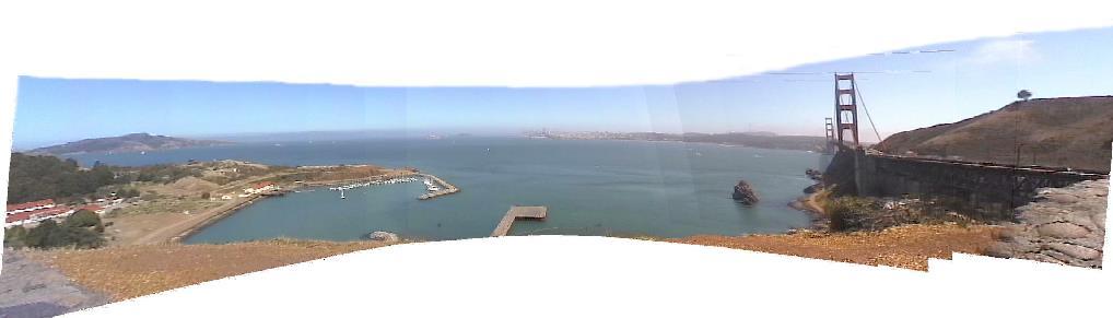


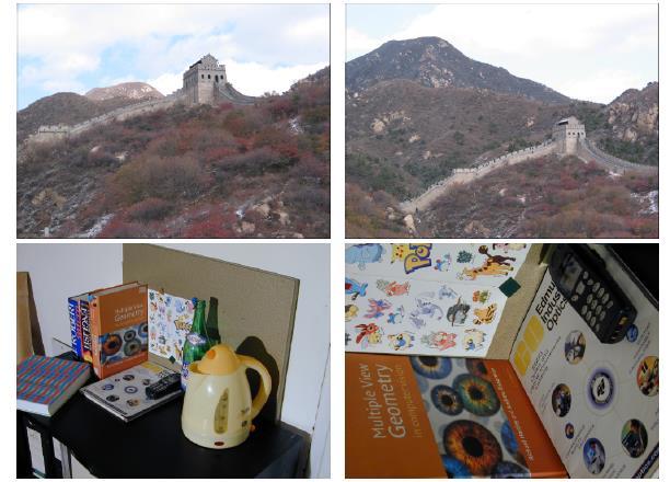
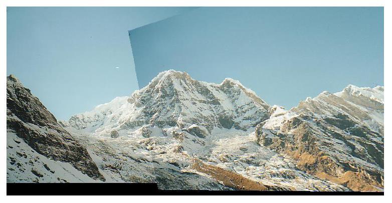
138 Example: Mosaicking with homographies 138

139 Recognizing Panoramas 139
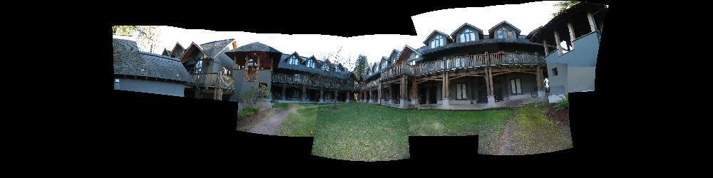
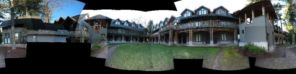
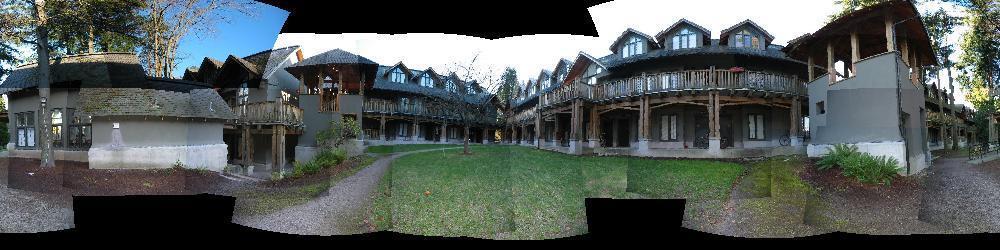

140 Recognizing Panoramas 140
141 THANK YOU!! 141
142 9/28 10/5 10/12 10/19 Liu Chang photosynth create account Take pictures Construct photosynth Markus Photomodeller Select one small object Make 3d model data Yang Yun PhotoCity Select one small object Make 3d model data Wang Ping PhotoCity Presentation file How to install & use Cygwin, bunder, Matlab CC Liu Pengxin Zhu Zi Jian 142 Wang Yuo Remove Perspective distortion Load image Choose feature points SIFT & ASIFT OpenCV CC PhotoTourism ARToolkit Camera Calibration PhotoTourism Matlab CC OpenCV CC Search others photosynth works Select one point in DSU, take pictures Projector Price? Matlab CC Lab Image Data SIFT Fundamental Matrix Remove PT OpenCV CC PT PhotoTourism ARToolkit Camera Calibration Fundamental Matrix M C C led lamp
143 Topics in Image Processing
144
145 145
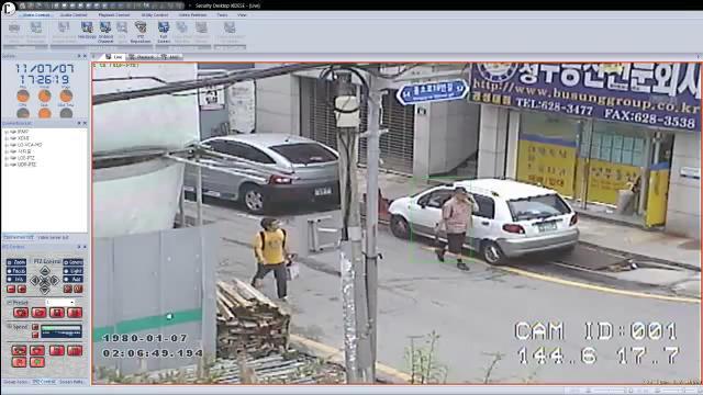
146 146
147
148


149 illisis 149


150 LYYN 150
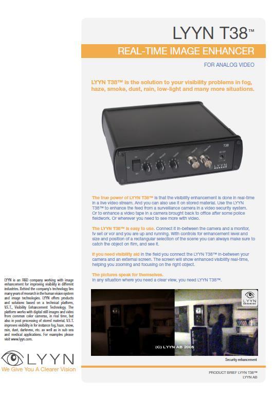
151


152 faceapi 152

153 Total Immersion - D Fusion Pro 153


154 D Fusion Pro - Markless Tracking 154
155 155

156 Monitoring System 156


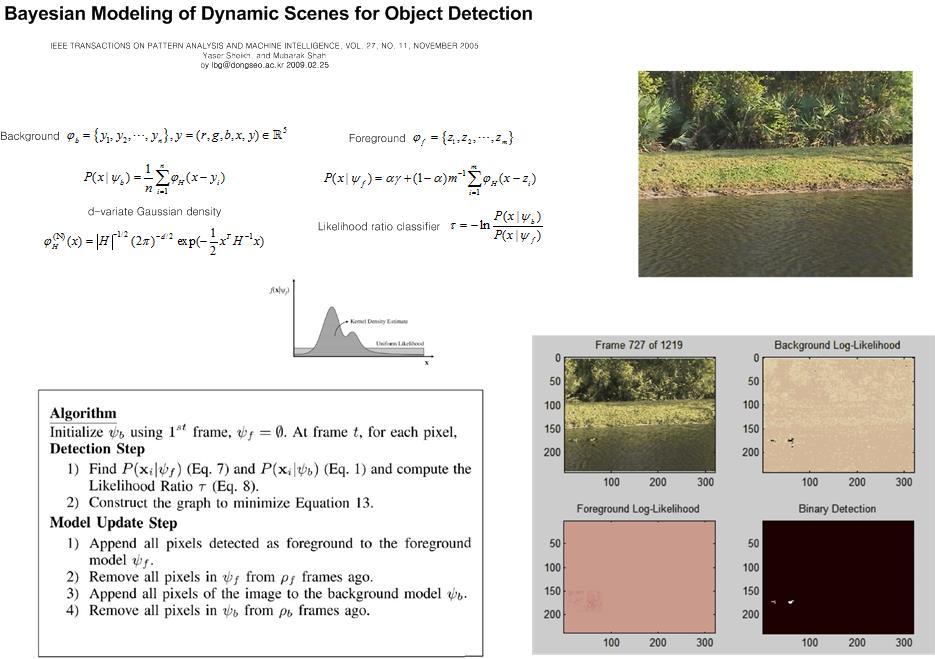
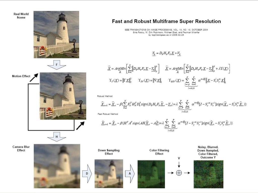
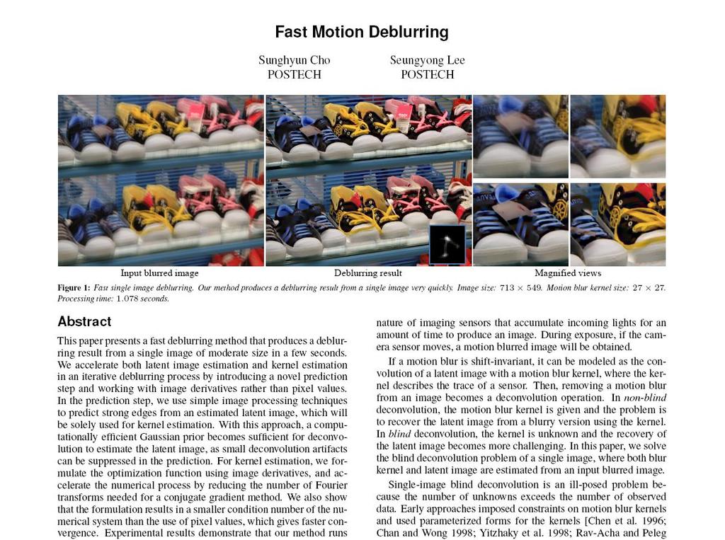
157 Scenarios Clear Vision - Denoising Motion Deblurring SuperResolution Panoramic View Background Modeling 157


158 Around View Monitor 158
159 Projective Transformations


160 Projective 2D Geometry 160
161 Projective transformations Definition: A projectivity is an invertible mapping h from P 2 to itself such that three points x 1,x 2,x 3 lie on the same line if and only if h(x 1 ),h(x 2 ),h(x 3 ) do. Theorem: A mapping h:p 2 P 2 is a projectivity if and only if there exist a non-singular 3x3 matrix H such that for any point in P 2 reprented by a vector x it is true that h(x)=hx Definition: Projective transformation x' x' x' h h h h h h h h h x x x or x' H x 8DOF projectivity=collineation=projective transformation=homography 161
162 Mapping between planes central projection may be expressed by x =Hx (application of theorem) 162

 (2 constraints/point, 8DOF 4 points needed) 23")
163 Removing projective distortion select four points in a plane with know coordinates x' 1 h11x h12y h13 x' 2 h21x h22y h x' y' x' h x h y h x' h x h y h x' y' h31x h32y h33 h11x h12y h13 h31x h32y h33 h21x h22y h (linear in h ij ) (2 constraints/point, 8DOF 4 points needed)
Epipolar Geometry class 11
 Epipolar Geometry class 11 Multiple View Geometry Comp 290-089 Marc Pollefeys Multiple View Geometry course schedule (subject to change) Jan. 7, 9 Intro & motivation Projective 2D Geometry Jan. 14, 16
3D reconstruction class 11
 3D reconstruction class 11 Multiple View Geometry Comp 290-089 Marc Pollefeys Multiple View Geometry course schedule (subject to change) Jan. 7, 9 Intro & motivation Projective 2D Geometry Jan. 14, 16
Projective 2D Geometry
 Projective D Geometry Multi View Geometry (Spring '08) Projective D Geometry Prof. Kyoung Mu Lee SoEECS, Seoul National University Homogeneous representation of lines and points Projective D Geometry Line
3D Photography: Epipolar geometry
 3D Photograph: Epipolar geometr Kalin Kolev, Marc Pollefes Spring 203 http://cvg.ethz.ch/teaching/203spring/3dphoto/ Schedule (tentative) Feb 8 Feb 25 Mar 4 Mar Mar 8 Mar 25 Apr Apr 8 Apr 5 Apr 22 Apr
Camera models and calibration
 Camera models and calibration Read tutorial chapter 2 and 3. http://www.cs.unc.edu/~marc/tutorial/ Szeliski s book pp.29-73 Schedule (tentative) 2 # date topic Sep.8 Introduction and geometry 2 Sep.25
Structure from motion
 Structure from motion Structure from motion Given a set of corresponding points in two or more images, compute the camera parameters and the 3D point coordinates?? R 1,t 1 R 2,t R 2 3,t 3 Camera 1 Camera
METR Robotics Tutorial 2 Week 2: Homogeneous Coordinates
 METR4202 -- Robotics Tutorial 2 Week 2: Homogeneous Coordinates The objective of this tutorial is to explore homogenous transformations. The MATLAB robotics toolbox developed by Peter Corke might be a
Epipolar Geometry Prof. D. Stricker. With slides from A. Zisserman, S. Lazebnik, Seitz
 Epipolar Geometry Prof. D. Stricker With slides from A. Zisserman, S. Lazebnik, Seitz 1 Outline 1. Short introduction: points and lines 2. Two views geometry: Epipolar geometry Relation point/line in two
Structure from motion
 Structure from motion Structure from motion Given a set of corresponding points in two or more images, compute the camera parameters and the 3D point coordinates?? R 1,t 1 R 2,t 2 R 3,t 3 Camera 1 Camera
Computer Vision I - Appearance-based Matching and Projective Geometry
 Computer Vision I - Appearance-based Matching and Projective Geometry Carsten Rother 05/11/2015 Computer Vision I: Image Formation Process Roadmap for next four lectures Computer Vision I: Image Formation
Structure from Motion
 11/18/11 Structure from Motion Computer Vision CS 143, Brown James Hays Many slides adapted from Derek Hoiem, Lana Lazebnik, Silvio Saverese, Steve Seitz, and Martial Hebert This class: structure from
Robot Vision: Projective Geometry
 Robot Vision: Projective Geometry Ass.Prof. Friedrich Fraundorfer SS 2018 1 Learning goals Understand homogeneous coordinates Understand points, line, plane parameters and interpret them geometrically
calibrated coordinates Linear transformation pixel coordinates
 1 calibrated coordinates Linear transformation pixel coordinates 2 Calibration with a rig Uncalibrated epipolar geometry Ambiguities in image formation Stratified reconstruction Autocalibration with partial
Multiple Views Geometry
 Multiple Views Geometry Subhashis Banerjee Dept. Computer Science and Engineering IIT Delhi email: suban@cse.iitd.ac.in January 2, 28 Epipolar geometry Fundamental geometric relationship between two perspective
Computer Vision I - Algorithms and Applications: Multi-View 3D reconstruction
 Computer Vision I - Algorithms and Applications: Multi-View 3D reconstruction Carsten Rother 09/12/2013 Computer Vision I: Multi-View 3D reconstruction Roadmap this lecture Computer Vision I: Multi-View
Camera Calibration. Schedule. Jesus J Caban. Note: You have until next Monday to let me know. ! Today:! Camera calibration
 Camera Calibration Jesus J Caban Schedule! Today:! Camera calibration! Wednesday:! Lecture: Motion & Optical Flow! Monday:! Lecture: Medical Imaging! Final presentations:! Nov 29 th : W. Griffin! Dec 1
Homogeneous Coordinates. Lecture18: Camera Models. Representation of Line and Point in 2D. Cross Product. Overall scaling is NOT important.
 Homogeneous Coordinates Overall scaling is NOT important. CSED44:Introduction to Computer Vision (207F) Lecture8: Camera Models Bohyung Han CSE, POSTECH bhhan@postech.ac.kr (",, ) ()", ), )) ) 0 It is
Projective geometry for Computer Vision
 Department of Computer Science and Engineering IIT Delhi NIT, Rourkela March 27, 2010 Overview Pin-hole camera Why projective geometry? Reconstruction Computer vision geometry: main problems Correspondence
3D Photography. Marc Pollefeys, Torsten Sattler. Spring 2015
 3D Photography Marc Pollefeys, Torsten Sattler Spring 2015 Schedule (tentative) Feb 16 Feb 23 Mar 2 Mar 9 Mar 16 Mar 23 Mar 30 Apr 6 Apr 13 Apr 20 Apr 27 May 4 May 11 May 18 Apr 6 Introduction Geometry,
Automatic Image Alignment (feature-based)
") Automatic Image Alignment (feature-based) Mike Nese with a lot of slides stolen from Steve Seitz and Rick Szeliski 15-463: Computational Photography Alexei Efros, CMU, Fall 2006 Today s lecture Feature
Automatic Image Alignment (feature-based) Mike Nese with a lot of slides stolen from Steve Seitz and Rick Szeliski 15-463: Computational Photography Alexei Efros, CMU, Fall 2006 Today s lecture Feature
Last lecture. Passive Stereo Spacetime Stereo
 Last lecture Passive Stereo Spacetime Stereo Today Structure from Motion: Given pixel correspondences, how to compute 3D structure and camera motion? Slides stolen from Prof Yungyu Chuang Epipolar geometry
Agenda. Rotations. Camera models. Camera calibration. Homographies
 Agenda Rotations Camera models Camera calibration Homographies D Rotations R Y = Z r r r r r r r r r Y Z Think of as change of basis where ri = r(i,:) are orthonormal basis vectors r rotated coordinate
Agenda. Rotations. Camera calibration. Homography. Ransac
 Agenda Rotations Camera calibration Homography Ransac Geometric Transformations y x Transformation Matrix # DoF Preserves Icon translation rigid (Euclidean) similarity affine projective h I t h R t h sr
Computer Vision I - Appearance-based Matching and Projective Geometry
 Computer Vision I - Appearance-based Matching and Projective Geometry Carsten Rother 01/11/2016 Computer Vision I: Image Formation Process Roadmap for next four lectures Computer Vision I: Image Formation
Vision par ordinateur
 Epipolar geometry π Vision par ordinateur Underlying structure in set of matches for rigid scenes l T 1 l 2 C1 m1 l1 e1 M L2 L1 e2 Géométrie épipolaire Fundamental matrix (x rank 2 matrix) m2 C2 l2 Frédéric
Lecture 9: Epipolar Geometry
 Lecture 9: Epipolar Geometry Professor Fei Fei Li Stanford Vision Lab 1 What we will learn today? Why is stereo useful? Epipolar constraints Essential and fundamental matrix Estimating F (Problem Set 2
Invariance of l and the Conic Dual to Circular Points C
 Invariance of l and the Conic Dual to Circular Points C [ ] A t l = (0, 0, 1) is preserved under H = v iff H is an affinity: w [ ] l H l H A l l v 0 [ t 0 v! = = w w] 0 0 v = 0 1 1 C = diag(1, 1, 0) is
3D Reconstruction from Two Views
 3D Reconstruction from Two Views Huy Bui UIUC huybui1@illinois.edu Yiyi Huang UIUC huang85@illinois.edu Abstract In this project, we study a method to reconstruct a 3D scene from two views. First, we extract
Multiple View Geometry in Computer Vision Second Edition
 Multiple View Geometry in Computer Vision Second Edition Richard Hartley Australian National University, Canberra, Australia Andrew Zisserman University of Oxford, UK CAMBRIDGE UNIVERSITY PRESS Contents
Stereo and Epipolar geometry
 Previously Image Primitives (feature points, lines, contours) Today: Stereo and Epipolar geometry How to match primitives between two (multiple) views) Goals: 3D reconstruction, recognition Jana Kosecka
Structure from Motion CSC 767
 Structure from Motion CSC 767 Structure from motion Given a set of corresponding points in two or more images, compute the camera parameters and the 3D point coordinates?? R,t R 2,t 2 R 3,t 3 Camera??
Unit 3 Multiple View Geometry
 Unit 3 Multiple View Geometry Relations between images of a scene Recovering the cameras Recovering the scene structure http://www.robots.ox.ac.uk/~vgg/hzbook/hzbook1.html 3D structure from images Recover
Index. 3D reconstruction, point algorithm, point algorithm, point algorithm, point algorithm, 253
 Index 3D reconstruction, 123 5+1-point algorithm, 274 5-point algorithm, 260 7-point algorithm, 255 8-point algorithm, 253 affine point, 43 affine transformation, 55 affine transformation group, 55 affine
3D Computer Vision. Structure from Motion. Prof. Didier Stricker
 3D Computer Vision Structure from Motion Prof. Didier Stricker Kaiserlautern University http://ags.cs.uni-kl.de/ DFKI Deutsches Forschungszentrum für Künstliche Intelligenz http://av.dfki.de 1 Structure
CS 664 Slides #9 Multi-Camera Geometry. Prof. Dan Huttenlocher Fall 2003
 CS 664 Slides #9 Multi-Camera Geometry Prof. Dan Huttenlocher Fall 2003 Pinhole Camera Geometric model of camera projection Image plane I, which rays intersect Camera center C, through which all rays pass
Computer Vision Projective Geometry and Calibration. Pinhole cameras
 Computer Vision Projective Geometry and Calibration Professor Hager http://www.cs.jhu.edu/~hager Jason Corso http://www.cs.jhu.edu/~jcorso. Pinhole cameras Abstract camera model - box with a small hole
Camera Geometry II. COS 429 Princeton University
 Camera Geometry II COS 429 Princeton University Outline Projective geometry Vanishing points Application: camera calibration Application: single-view metrology Epipolar geometry Application: stereo correspondence
55:148 Digital Image Processing Chapter 11 3D Vision, Geometry
 55:148 Digital Image Processing Chapter 11 3D Vision, Geometry Topics: Basics of projective geometry Points and hyperplanes in projective space Homography Estimating homography from point correspondence
Index. 3D reconstruction, point algorithm, point algorithm, point algorithm, point algorithm, 263
 Index 3D reconstruction, 125 5+1-point algorithm, 284 5-point algorithm, 270 7-point algorithm, 265 8-point algorithm, 263 affine point, 45 affine transformation, 57 affine transformation group, 57 affine
Stereo Vision. MAN-522 Computer Vision
 Stereo Vision MAN-522 Computer Vision What is the goal of stereo vision? The recovery of the 3D structure of a scene using two or more images of the 3D scene, each acquired from a different viewpoint in
BIL Computer Vision Apr 16, 2014
 BIL 719 - Computer Vision Apr 16, 2014 Binocular Stereo (cont d.), Structure from Motion Aykut Erdem Dept. of Computer Engineering Hacettepe University Slide credit: S. Lazebnik Basic stereo matching algorithm
3D Computer Vision II. Reminder Projective Geometry, Transformations
 3D Computer Vision II Reminder Projective Geometry, Transformations Nassir Navab" based on a course given at UNC by Marc Pollefeys & the book Multiple View Geometry by Hartley & Zisserman" October 21,
Week 2: Two-View Geometry. Padua Summer 08 Frank Dellaert
 Week 2: Two-View Geometry Padua Summer 08 Frank Dellaert Mosaicking Outline 2D Transformation Hierarchy RANSAC Triangulation of 3D Points Cameras Triangulation via SVD Automatic Correspondence Essential
Rectification and Distortion Correction
 Rectification and Distortion Correction Hagen Spies March 12, 2003 Computer Vision Laboratory Department of Electrical Engineering Linköping University, Sweden Contents Distortion Correction Rectification
Feature Based Registration - Image Alignment
 Feature Based Registration - Image Alignment Image Registration Image registration is the process of estimating an optimal transformation between two or more images. Many slides from Alexei Efros http://graphics.cs.cmu.edu/courses/15-463/2007_fall/463.html
55:148 Digital Image Processing Chapter 11 3D Vision, Geometry
 55:148 Digital Image Processing Chapter 11 3D Vision, Geometry Topics: Basics of projective geometry Points and hyperplanes in projective space Homography Estimating homography from point correspondence
Multiple View Geometry in Computer Vision
 Multiple View Geometry in Computer Vision Prasanna Sahoo Department of Mathematics University of Louisville 1 Projective 3D Geometry (Back to Chapter 2) Lecture 6 2 Singular Value Decomposition Given a
Multiple View Geometry in computer vision
 Multiple View Geometry in computer vision Chapter 8: More Single View Geometry Olaf Booij Intelligent Systems Lab Amsterdam University of Amsterdam, The Netherlands HZClub 29-02-2008 Overview clubje Part
Structure from Motion
 Structure from Motion Outline Bundle Adjustment Ambguities in Reconstruction Affine Factorization Extensions Structure from motion Recover both 3D scene geoemetry and camera positions SLAM: Simultaneous
A Summary of Projective Geometry
 A Summary of Projective Geometry Copyright 22 Acuity Technologies Inc. In the last years a unified approach to creating D models from multiple images has been developed by Beardsley[],Hartley[4,5,9],Torr[,6]
Projective geometry, camera models and calibration
 Projective geometry, camera models and calibration Subhashis Banerjee Dept. Computer Science and Engineering IIT Delhi email: suban@cse.iitd.ac.in January 6, 2008 The main problems in computer vision Image
Part 0. The Background: Projective Geometry, Transformations and Estimation
 Part 0 The Background: Projective Geometry, Transformations and Estimation La reproduction interdite (The Forbidden Reproduction), 1937, René Magritte. Courtesy of Museum Boijmans van Beuningen, Rotterdam.
Augmented Reality II - Camera Calibration - Gudrun Klinker May 11, 2004
 Augmented Reality II - Camera Calibration - Gudrun Klinker May, 24 Literature Richard Hartley and Andrew Zisserman, Multiple View Geometry in Computer Vision, Cambridge University Press, 2. (Section 5,
Computer Vision. 2. Projective Geometry in 3D. Lars Schmidt-Thieme
 Computer Vision 2. Projective Geometry in 3D Lars Schmidt-Thieme Information Systems and Machine Learning Lab (ISMLL) Institute for Computer Science University of Hildesheim, Germany 1 / 26 Syllabus Mon.
Computing F class 13. Multiple View Geometry. Comp Marc Pollefeys
 Computing F class 3 Multiple View Geometr Comp 90-089 Marc Pollefes Multiple View Geometr course schedule (subject to change) Jan. 7, 9 Intro & motivation Projective D Geometr Jan. 4, 6 (no class) Projective
CS231A Midterm Review. Friday 5/6/2016
 CS231A Midterm Review Friday 5/6/2016 Outline General Logistics Camera Models Non-perspective cameras Calibration Single View Metrology Epipolar Geometry Structure from Motion Active Stereo and Volumetric
Two-view geometry Computer Vision Spring 2018, Lecture 10
 Two-view geometry http://www.cs.cmu.edu/~16385/ 16-385 Computer Vision Spring 2018, Lecture 10 Course announcements Homework 2 is due on February 23 rd. - Any questions about the homework? - How many of
CS231M Mobile Computer Vision Structure from motion
 CS231M Mobile Computer Vision Structure from motion - Cameras - Epipolar geometry - Structure from motion Pinhole camera Pinhole perspective projection f o f = focal length o = center of the camera z y
CS-9645 Introduction to Computer Vision Techniques Winter 2019
 Table of Contents Projective Geometry... 1 Definitions...1 Axioms of Projective Geometry... Ideal Points...3 Geometric Interpretation... 3 Fundamental Transformations of Projective Geometry... 4 The D
CSE 252B: Computer Vision II
 CSE 252B: Computer Vision II Lecturer: Serge Belongie Scribe: Sameer Agarwal LECTURE 1 Image Formation 1.1. The geometry of image formation We begin by considering the process of image formation when a
COMPARATIVE STUDY OF DIFFERENT APPROACHES FOR EFFICIENT RECTIFICATION UNDER GENERAL MOTION
 COMPARATIVE STUDY OF DIFFERENT APPROACHES FOR EFFICIENT RECTIFICATION UNDER GENERAL MOTION Mr.V.SRINIVASA RAO 1 Prof.A.SATYA KALYAN 2 DEPARTMENT OF COMPUTER SCIENCE AND ENGINEERING PRASAD V POTLURI SIDDHARTHA
Epipolar Geometry and the Essential Matrix
 Epipolar Geometry and the Essential Matrix Carlo Tomasi The epipolar geometry of a pair of cameras expresses the fundamental relationship between any two corresponding points in the two image planes, and
Camera model and calibration
 and calibration AVIO tristan.moreau@univ-rennes1.fr Laboratoire de Traitement du Signal et des Images (LTSI) Université de Rennes 1. Mardi 21 janvier 1 AVIO tristan.moreau@univ-rennes1.fr and calibration
Structure from Motion. Introduction to Computer Vision CSE 152 Lecture 10
 Structure from Motion CSE 152 Lecture 10 Announcements Homework 3 is due May 9, 11:59 PM Reading: Chapter 8: Structure from Motion Optional: Multiple View Geometry in Computer Vision, 2nd edition, Hartley
Computer Vision cmput 428/615
 Computer Vision cmput 428/615 Basic 2D and 3D geometry and Camera models Martin Jagersand The equation of projection Intuitively: How do we develop a consistent mathematical framework for projection calculations?
Epipolar Geometry and Stereo Vision
 Epipolar Geometry and Stereo Vision Computer Vision Jia-Bin Huang, Virginia Tech Many slides from S. Seitz and D. Hoiem Last class: Image Stitching Two images with rotation/zoom but no translation. X x
Structure from Motion
 /8/ Structure from Motion Computer Vision CS 43, Brown James Hays Many slides adapted from Derek Hoiem, Lana Lazebnik, Silvio Saverese, Steve Seitz, and Martial Hebert This class: structure from motion
Structure from motion
 Structure from motion Structure from motion Given a set of corresponding points in two or more images, compute the camera parameters and the 3D point coordinates?? R 1,t 1 R 2,t 2 R 3,t 3 Camera 1 Camera
Recovering structure from a single view Pinhole perspective projection
 EPIPOLAR GEOMETRY The slides are from several sources through James Hays (Brown); Silvio Savarese (U. of Michigan); Svetlana Lazebnik (U. Illinois); Bill Freeman and Antonio Torralba (MIT), including their
C / 35. C18 Computer Vision. David Murray. dwm/courses/4cv.
 C18 2015 1 / 35 C18 Computer Vision David Murray david.murray@eng.ox.ac.uk www.robots.ox.ac.uk/ dwm/courses/4cv Michaelmas 2015 C18 2015 2 / 35 Computer Vision: This time... 1. Introduction; imaging geometry;
Epipolar geometry. x x
 Two-view geometry Epipolar geometry X x x Baseline line connecting the two camera centers Epipolar Plane plane containing baseline (1D family) Epipoles = intersections of baseline with image planes = projections
Visual Recognition: Image Formation
 Visual Recognition: Image Formation Raquel Urtasun TTI Chicago Jan 5, 2012 Raquel Urtasun (TTI-C) Visual Recognition Jan 5, 2012 1 / 61 Today s lecture... Fundamentals of image formation You should know
Instance-level recognition I. - Camera geometry and image alignment
 Reconnaissance d objets et vision artificielle 2011 Instance-level recognition I. - Camera geometry and image alignment Josef Sivic http://www.di.ens.fr/~josef INRIA, WILLOW, ENS/INRIA/CNRS UMR 8548 Laboratoire
More on single-view geometry class 10
 More on single-view geometry class 10 Multiple View Geometry Comp 290-089 Marc Pollefeys Multiple View Geometry course schedule (subject to change) Jan. 7, 9 Intro & motivation Projective 2D Geometry Jan.
Multiple View Geometry in Computer Vision
 Multiple View Geometry in Computer Vision Prasanna Sahoo Department of Mathematics University of Louisville 1 More on Single View Geometry Lecture 11 2 In Chapter 5 we introduced projection matrix (which
Projective geometry for 3D Computer Vision
 Subhashis Banerjee Computer Science and Engineering IIT Delhi Dec 16, 2015 Overview Pin-hole camera Why projective geometry? Reconstruction Computer vision geometry: main problems Correspondence problem:
CS201 Computer Vision Camera Geometry
 CS201 Computer Vision Camera Geometry John Magee 25 November, 2014 Slides Courtesy of: Diane H. Theriault (deht@bu.edu) Question of the Day: How can we represent the relationships between cameras and the
MAPI Computer Vision. Multiple View Geometry
 MAPI Computer Vision Multiple View Geometry Geometry o Multiple Views 2- and 3- view geometry p p Kpˆ [ K R t]p Geometry o Multiple Views 2- and 3- view geometry Epipolar Geometry The epipolar geometry
Robust Geometry Estimation from two Images
 Robust Geometry Estimation from two Images Carsten Rother 09/12/2016 Computer Vision I: Image Formation Process Roadmap for next four lectures Computer Vision I: Image Formation Process 09/12/2016 2 Appearance-based
EXAM SOLUTIONS. Image Processing and Computer Vision Course 2D1421 Monday, 13 th of March 2006,
 School of Computer Science and Communication, KTH Danica Kragic EXAM SOLUTIONS Image Processing and Computer Vision Course 2D1421 Monday, 13 th of March 2006, 14.00 19.00 Grade table 0-25 U 26-35 3 36-45
Part I: Single and Two View Geometry Internal camera parameters
 !! 43 1!???? Imaging eometry Multiple View eometry Perspective projection Richard Hartley Andrew isserman O p y VPR June 1999 where image plane This can be written as a linear mapping between homogeneous
Visual Odometry. Features, Tracking, Essential Matrix, and RANSAC. Stephan Weiss Computer Vision Group NASA-JPL / CalTech
 Visual Odometry Features, Tracking, Essential Matrix, and RANSAC Stephan Weiss Computer Vision Group NASA-JPL / CalTech Stephan.Weiss@ieee.org (c) 2013. Government sponsorship acknowledged. Outline The
N-Views (1) Homographies and Projection
 Homographies and Projection") CS 4495 Computer Vision N-Views (1) Homographies and Projection Aaron Bobick School of Interactive Computing Administrivia PS 2: Get SDD and Normalized Correlation working for a given windows size say
CS 4495 Computer Vision N-Views (1) Homographies and Projection Aaron Bobick School of Interactive Computing Administrivia PS 2: Get SDD and Normalized Correlation working for a given windows size say
Multiple View Geometry in Computer Vision
 Multiple View Geometry in Computer Vision Prasanna Sahoo Department of Mathematics University of Louisville 1 Structure Computation Lecture 18 March 22, 2005 2 3D Reconstruction The goal of 3D reconstruction
3D Geometry and Camera Calibration
 3D Geometry and Camera Calibration 3D Coordinate Systems Right-handed vs. left-handed x x y z z y 2D Coordinate Systems 3D Geometry Basics y axis up vs. y axis down Origin at center vs. corner Will often
Pin Hole Cameras & Warp Functions
 Pin Hole Cameras & Warp Functions Instructor - Simon Lucey 16-423 - Designing Computer Vision Apps Today Pinhole Camera. Homogenous Coordinates. Planar Warp Functions. Motivation Taken from: http://img.gawkerassets.com/img/18w7i1umpzoa9jpg/original.jpg
Camera model and multiple view geometry
 Chapter Camera model and multiple view geometry Before discussing how D information can be obtained from images it is important to know how images are formed First the camera model is introduced and then
Auto-calibration. Computer Vision II CSE 252B
 Auto-calibration Computer Vision II CSE 252B 2D Affine Rectification Solve for planar projective transformation that maps line (back) to line at infinity Solve as a Householder matrix Euclidean Projective
Automatic Image Alignment
 Automatic Image Alignment Mike Nese with a lot of slides stolen from Steve Seitz and Rick Szeliski 15-463: Computational Photography Alexei Efros, CMU, Fall 2010 Live Homography DEMO Check out panoramio.com
Automatic Image Alignment
 Automatic Image Alignment with a lot of slides stolen from Steve Seitz and Rick Szeliski Mike Nese CS194: Image Manipulation & Computational Photography Alexei Efros, UC Berkeley, Fall 2018 Live Homography
Motion Estimation and Optical Flow Tracking
 Image Matching Image Retrieval Object Recognition Motion Estimation and Optical Flow Tracking Example: Mosiacing (Panorama) M. Brown and D. G. Lowe. Recognising Panoramas. ICCV 2003 Example 3D Reconstruction
Robotics - Projective Geometry and Camera model. Matteo Pirotta
 Robotics - Projective Geometry and Camera model Matteo Pirotta pirotta@elet.polimi.it Dipartimento di Elettronica, Informazione e Bioingegneria Politecnico di Milano 14 March 2013 Inspired from Simone
EM225 Projective Geometry Part 2
 EM225 Projective Geometry Part 2 eview In projective geometry, we regard figures as being the same if they can be made to appear the same as in the diagram below. In projective geometry: a projective point
Lecture 10: Multi-view geometry
 Lecture 10: Multi-view geometry Professor Stanford Vision Lab 1 What we will learn today? Review for stereo vision Correspondence problem (Problem Set 2 (Q3)) Active stereo vision systems Structure from
Multi-view geometry problems
 Multi-view geometry Multi-view geometry problems Structure: Given projections o the same 3D point in two or more images, compute the 3D coordinates o that point? Camera 1 Camera 2 R 1,t 1 R 2,t 2 Camera
Structure from Motion. Prof. Marco Marcon
 Structure from Motion Prof. Marco Marcon Summing-up 2 Stereo is the most powerful clue for determining the structure of a scene Another important clue is the relative motion between the scene and (mono)
Homographies and RANSAC
 Homographies and RANSAC Computer vision 6.869 Bill Freeman and Antonio Torralba March 30, 2011 Homographies and RANSAC Homographies RANSAC Building panoramas Phototourism 2 Depth-based ambiguity of position
CEE598 - Visual Sensing for Civil Infrastructure Eng. & Mgmt.
 CEE598 - Visual Sensing for Civil Infrastructure Eng. & Mgmt. Session 4 Affine Structure from Motion Mani Golparvar-Fard Department of Civil and Environmental Engineering 329D, Newmark Civil Engineering
Robotics - Single view, Epipolar geometry, Image Features. Simone Ceriani
 Robotics - Single view, Epipolar geometry, Image Features Simone Ceriani ceriani@elet.polimi.it Dipartimento di Elettronica e Informazione Politecnico di Milano 12 April 2012 2/67 Outline 1 Pin Hole Model
CS231A Course Notes 4: Stereo Systems and Structure from Motion
 CS231A Course Notes 4: Stereo Systems and Structure from Motion Kenji Hata and Silvio Savarese 1 Introduction In the previous notes, we covered how adding additional viewpoints of a scene can greatly enhance