Department of Electrical and Computer Systems Engineering

Transcription

1 Department of Electrical and Computer Systems Engineering Technical Report MECSE Scan Matching in Polar Coordinates with Application to SLAM A. Diosi and L. Kleeman

2 Scan Matching in Polar Coordinates with Application to SLAM Albert Diosi and Lindsay Kleeman ARC Centre for Perceptive and Intelligent Machines in Complex Environments Department of Electrical and Computer Systems Engineering Monash University, Clayton, VIC 3168, Australia July 22, 2005 Abstract This report presents a novel method for 2D laser scan matching called Polar Scan Matching (PSM). The method belongs to the family of point to point matching approaches. Our method avoids searching for point associations by simply matching points with the same bearing. This association rule enables the construction of an algorithm faster than the iterative closest point (ICP). Firstly the PSM approach is tested with simulated laser scans. Then the accuracy of our matching algorithm is evaluated from real laser scans from known relative positions to establish a ground truth. Furthermore, to demonstrate the practical usability of the new PSM approach, experimental results from a Kalman filter implementation of simultaneous localization and mapping (SLAM) are provided. 1

3 Contents 1 Introduction 3 2 Scan Preprocessing Median Filtering Long Range Measurements Segmentation Motion Tracking Current Scan Pose in Reference Scan Coordinate Frame Scan Matching Scan Projection Translation Estimation Pose Estimation in Cartesian Frame Orientation Estimation Error Estimation Covariance Estimate of Weighted Least Squares Heuristic Covariance Estimation SLAM using Polar Scan Matching 26 6 Experimental Results Simple Implementation of ICP Simulated Room Ground Thruth Experiment Convergence Map SLAM Extensions to 3D 48 8 Discussion 48

4 1 INTRODUCTION 3 1 Introduction Localization and map making is an important function of mobile robots. One possible way to assist with this functionality is to use laser scan matching. In laser scan matching, the position and orientation or pose of the current scan is sought with respect to a reference laser scan by adjusting the pose of the current scan until the best overlap with the reference scan is achieved. In the literature there are methods for 2D and 3D scan matching. This report restricts discussion to 2D laser scan matching. Scan matching approaches can be local [Lu and Milios, 1997] or global [Tomono, 2004]. When performing local scan matching, two scans are matched while starting from an initial pose estimate. When performing global scan matching the current scan is aligned with respect to a map or a database of scans without the need to supply an initial pose estimate. Scan matching approaches also can be categorized based on their association method such as feature to feature, point to feature and point to point. In feature to feature matching approaches, features such as line segments [Gutmann, 2000], corners or range extrema [Lingemann et al., 2004] are extracted from laser scans, and then matched. Such approaches interpret laser scans and require the presence of chosen features in the environment. In point to feature approaches, such as one of the earliest by Cox [1991], the points of a scan are matched to features such as lines. The line features can be part of a predefined map. Features can be more abstract as in [Biber and Straßer, 2003], where features are Gaussian distributions with their mean and variance calculated from scan points falling into cells of a grid. Point to point matching approaches such as the approach presented in this report, do not require the environment to be structured or contain predefined features. Examples of point to point matching approaches are the following: iterative closest point (ICP), iterative matching range point (IMRP) and the popular iterative dual correspondence (IDC). Besl and Mac Kay [1992] proposed ICP, where for each point of the current scan, the point with the smallest Euclidean distance in the reference scan is selected. IMPR was proposed by Lu and Milios [1997], where corresponding points are selected by choosing a point which has the matching range from the center of the reference scan s coordinate system. IDC, also proposed by Lu and Milios [1997] combines ICP and IMRP by using the ICP to calculate translation and IMPR to calculate rotation. The mentioned point to point methods can find the correct pose of the current scan in one step provided the correct associations are chosen. Since the correct associations are unknown, several iterations are performed. Matching may not always converge to the correct pose, since they can get stuck in a local minima. Due to the applied association rules, matching points have to be searched across 2 scans, resulting in O(n 2 ) com-

5 1 INTRODUCTION 4 plexity 1, where n is the number of scan points. All three approaches operate in a Cartesian coordinate frame and therefore do not take advantage of the native polar coordinate system of a laser scan. However, as shown later in this report, a scan matching algorithm working in the polar coordinate system of a laser scanner can eliminate the search for corresponding points thereby achieving O(n) computational complexity for translation estimation. O(n) computational complexity is also achievable for orientation estimation if a limited orientation estimation accuracy is acceptable. These point to point matching algorithms apply a so called projection filter [Gutmann, 2000] prior to matching. The objective of this filter is to remove those points from the reference and current scan not likely to have a corresponding point. The computational complexity of this filter is also O(n 2 ). There are other scan matching approaches such as the method of Weiss and Puttkamer [1995]. Here for both reference and current scans, an angle-histogram of the orientation of line segments connecting consecutive points is generated. The orientation of the current scan with respect to the reference scan is obtained by finding the phase with the maximum cross correlation of the 2 angle histograms. The translation is found similarly by calculating x and y histograms, and calculating cross correlations. In scan matching, not all approaches use only that information in a scan, which describes where objects are located. Thrun et al. [2000] in their scan matching method utilize the idea, that free space in a scan is unlikely to be occupied in future scans. In scan matching another important task, apart from finding the current scans pose, is the estimation of the quality of the match. Lu and Milios [1997] calculate the uncertainty of the match results by assuming white Gaussian noise in the x,y coordinates of scan points. This implicitly assumes that correct associations are made that results in optimistic error estimates, especially in corridors. Bengtsson and Baerveldt in [2001] developed more realistic approaches. In their first approach the pose covariance matrix is estimated from the Hessian of the scan matching error function. In their second approach, the covariance matrix is estimated off-line by simulating current scans and matching them to the reference scan. Mapping with scan matching has been done for example by minimizing an energy function [Lu, 1995], using a combination of maximum likelihood with posterior estimation [Thrun et al., 2000], using local registration and global cor- 1 Lu and Milios [1997] claim that the IDC is of O(n) complexity if the search for corresponding points is restricted to a window consisting of a fixed number of points. However if the angular resolution of laser scans is increased then the use of such a search window results in a decrease in the performance of the IDC due to the shrinking size of the search window expressed in angles. Therefore as it is correctly pointed out in [Gutmann, 2000] the computational complexity of IDC is O(n 2 ).

6 2 SCAN PREPROCESSING 5 relation [Gutmann, 2000] and using FastSLAM [Hähnel et al., 2003]. A Kalman filter implementation can be found in [Bosse et al., 2004]. In this report the Polar Scan Matching (PSM) approach is described which works in the laser scanner s polar coordinate system, therefore taking advantage of the structure of the laser measurements by eliminating the search for corresponding points. It assumed that in the 2D laser measurements range readings are ordered by their bearings. Laser range measurements of current and reference scans are associated with each other using the matching bearing rule, which makes translation estimation of the PSM approach O(n) complexity unlike IDC s O(n 2 ). The orientation estimation s computational complexity is also O(n) if limited accuracy is acceptable, otherwise O(kn), where k is proportional to the number of range readings per unit angle i.e. to the angular resolution of the scan. Note that k is introduced to differentiate between increasing the number of scan points by increasing the field of view or the angular resolution of the laser range finder. An O(mn) complexity scan projection algorithm working in polar coordinates is also described in this report. The variable m equals to one added to the maximum number of objects occluding each other in the current scan viewed from the reference scan s pose. However this projection filter is of O(n) complexity if no occlusions occur in the scan, therefore being more efficient than that of [Gutmann, 2000]. The rest of this report is organized as follows; first scan preprocessing steps, followed by the PSM algorithm is described. A heuristic scan match error model is presented next followed by a Kalman filter SLAM implementation utilizing our scan matching approach. Details of experimental results follow that include simulation, ground truth measurements and an implementation of SLAM. SLAM results with PSM are compared with results from SLAM using laser range finder and advanced sonar arrays [Diosi et al., 2005; Diosi and Kleeman, 2004]. Finally conclusions and future work are presented. Part of the work presented in this report is published as [Diosi and Kleeman, 2005]. 2 Scan Preprocessing Prior to matching, the current and the reference scans are preprocessed. Preprocessing helps to remove erroneous measurements, clutter or to group measurements of the same object to increase the accuracy and robustness of scan matching. In fig. 1 a laser scan is depicted in a Cartesian coordinate system. Corresponding raw range measurements are shown in fig. 2. Laser scans can have points which are not suitable matching. Such points are: Points representing moving objects such as the legs of a person in fig 1. Table and chair legs are also such points, since they are less likely to be

7 2 SCAN PREPROCESSING 6 person mixed pixel hanging cable Figure 1: Laser scan in a Cartesian coordinate frame. Grid is 1m. hanging cable mixed pixel person Figure 2: Scan of fig. 1 in the laser s polar coordinate frame. Horizontal grid size is 10, vertical grid size is 1m.

8 2 SCAN PREPROCESSING 7 static in the long term. Mixed pixels. At range discontinuities laser scanners often generate measurements which are located in the free space between two objects [Ye and Borenstein, 2002]. Measurements with maximum range. Such readings are returned, when there is no object withing the range of the scanner. Also some surfaces (for example clean clear glass) do not illuminate well and show a laser spot, therefore they can appear as measurements with maximum range. Instead of only removing range readings which are out of the range of the sensor, it was found useful to artificially restrict the sensor to a distance PM MAX RANGE = 10m (1) and disregard (tag) any more distant readings. When having a sensor with 1 angular resolution, the minimum distance between two readings at 10 meters is 17cm. A large distance between neighboring points complicates the segmentation of scans, since if the distance between measured points is large it is hard to decide if the points belong to the same object. Interpolating between two neighboring points belonging to 2 different objects can be a source of error. In addition by artificially restricting the range of the sensor, difficulties may be introduced in large rooms with a lot of open space. In the following subsections we will focus on how to exclude these unwanted points from the scan matching process. 2.1 Median Filtering Median filters are used to replace outliers with suitable measurements [Gutmann, 2000]. After the application of a median filter to the range readings, objects such as chair and table legs are likely to be removed. Similarly to [Gutmann, 2000], a window size of PM MEDIAN WINDOW = 5 (2) for the median filter was found satisfactory since it can replace at most 2 neighborings outliers. Mixed pixels are unlikely to be replaced by a median filter. The result after applying median filter to the scan of fig. 1 can be seen in figures 3 and 4. From fig. 4 it is clear, that at least 4 spikes were replaced, but all the mixed pixels still remain.

9 2 SCAN PREPROCESSING 8 mixed pixel Figure 3: Laser scan of fig. 1 in a Cartesian coordinate frame after median filtering. Grid is 1m. mixed pixel Figure 4: Scan of fig. 1 in the laser s polar coordinate frame after median filtering. Horizontal grid size is 10, vertical grid size is 1m.

10 2 SCAN PREPROCESSING 9 Figure 5: Laser scan of fig. 3 in a Cartesian coordinate frame after segmentation. Grid is 1m. Segments are assigned numbers. 0 is assigned to segments having only one point. 2.2 Long Range Measurements After the application of a median filter all points further than a threshold PM MAX RANGE are tagged. These tagged points are used only in segmentation described next and not in scan matching. Range measurements larger than a PM MAX RANGE are not used in the scan matching because distance between such measurements is large, which makes it hard to decide if they belong to the same object or not. 2.3 Segmentation Segmenting range measurements can have two advantages. The first advantage is that interpolation between 2 separate objects can be avoided if one knows that the objects are separate. Such interpolation is useful when one wants to know how a scan would look from a different location (scan projection). The second advantage is that if laser scans are segmented and the segments are tracked in consecutive scans then certain types of moving objects can be identified. Tracking moving objects can make scan matching more robust. Two criteria are used in the segmentation process. According to the first criterion, a range reading, not differing more than PM MAX DIFF = 20cm (3)

11 2 SCAN PREPROCESSING 10 Figure 6: Scan of fig. 3 in the laser s polar coordinate frame after segmentation. Horizontal grid size is 10, vertical grid size is 1m. Segments are assigned numbers. 0 is assigned to segments having only one point. from the previous range reading, belongs to the same segment. This criterion fails to correctly segment out points which are for example on a wall oriented towards the laser. Therefore a second criterion is also applied according to which if 3 consecutive range readings lie approximately on the same polar line, then they belong to the same segment. Note that a mixed pixel can only then connect two objects if the distance between first object and mixed pixel and second object and mixed pixel is less than PM MAX DIFF. Tagged range readings also break segments. Segmentation results can be seen in fig. 5 and 6. Different segments are assigned different numbers, except 0, which is assigned to segments consisting of only one point. Segments assigned 0 are also tagged, therefore they are not used in the scan matching process. Note that most of the mixed pixels get assigned 0. Note that this simple segmentation is of O(n) complexity. 2.4 Motion Tracking One of the problems of point to point scan matching is that moving objects can cause wrong associations thus reducing the accuracy of the scan matching results, or can even cause divergence. It is therefore advisable to track and tag moving objects in laser scans. Motion tracking constitutes future work and is beyond the scope of this report.

12 2 SCAN PREPROCESSING 11 Y Ref. scan frame Cur. scan frame Laser centre Odometry centre Robot ref. frame T1 y TL y x reference x T3 T2 y TLy x x current World frame X Figure 7: Reference and current coordinate frames. 2.5 Current Scan Pose in Reference Scan Coordinate Frame To make scan matching simpler, let us set the goal of scan matching to find the position and orientation (or pose) of the current laser scan s coordinate frame with respect to the reference scans coordinate frame (see fig. 7). Otherwise the introduction of a world frame in which to relate the current and reference frame would make the equations describing the relation of current and reference scan points more complicated. The reference scans coordinate frame is the coordinate frame of the laser scanner at the reference location. To find out the position and orientation of the current frame with respect to reference frame, from fig. 7 we can write: T 1 T L T 3 = T 2 T L (4) where T 1 is the homogeneous transformation matrix from robot frame at reference location to world frame, T 2 is the transformation from robot frame at current location to world frame, T 3 is the transformation from current laser scan frame to reference laser scan frame and T L is the transformation from laser frame into robot frame. With the multiplication of the matrices it is assumed that coordinates of points are stored in column vectors therefore the transformations are applied from right to left. From (4), the transformation from current into reference frame is: T 3 = T 1 L T 1 1 T 2T L. (5)

13 3 SCAN MATCHING 12 If (x rr,y rr,θ rr ) describes the robot s pose at the reference location expressed in world frame, (x cr,y cr,θ cr ) describes the robot pose the current location expressed in world frame, (x c,y c,θ c ) describes the laser scanner s pose at the current location expressed in the reference frame, and if the laser scanners pose is described with (x l,y l,θ l ) in the robots frame, then: T 3 = T L = cosθ c sinθ c x c sinθ c cosθ c y c cosθ l sinθ l x l sinθ l cosθ l y l T 1 = T 2 = cosθ rr sinθ rr x rr sinθ rr cosθ rr y rr cosθ cr sinθ cr x cr sinθ cr cosθ cr y cr By substituting (6) into (5) and comparing the left and right sides, the current pose (x c,y c,θ c ) expressed in the reference frame can be determined as: (6) θ c = θ cr θ rr (7) x c = x l (cosβ cosθ l ) + y l (sinβ sinθ l ) + (x cr x rr )cos γ + (y cr y rr )sinγ (8) y c = x l (sin β sinθ l ) + y l (cos β cosθ l ) (x cr x rr )sin γ + (y cr y rr )cos γ (9) where β = θ l + θ rr θ cr and γ = θ l + θ rr. 3 Scan Matching The laser scan matching method described next aligns the current scan with respect to the reference scan so that the sum of square range residuals is minimized. It is assumed that an initial pose of the current scan is given, expressed in the coordinate frame of the reference scan. The coordinate frame of a laser scan is centered at the point of rotation of the mirror of a laser scanner. The X axis or zero angle of the laser s Cartesian coordinate system coincides with the direction of the first reported range measurement. The current scan is described as C = (x c,y c,θ c,{r ci,φ ci } n i=1 ), where x c,y c,θ c describe position and orientation, {r ci,φ ci } n i=1 describe n range measurements r ci at bearings φ ci, expressed in the current scan s coordinate system. {r ci,φ ci } n i=1 are ordered by the bearings in ascending order as they are received from a SICK laser scanner. The reference scan is described as R = {r ri,φ ri } n i=1. Note that if bearings where range measurements are taken are unchanged in current and reference scans then φ ri = φ ci. The scan matching works as follows: after preprocessing the scans, scan projection followed by a translation estimation or orientation estimation are iterated. In

14 3 SCAN MATCHING 13 Figure 8: a) projection of measured points taken at C to location R. b) points projected to R shown in polar coordinates. Dashed lines represent bearings which the scanner would have sampled. the polar scan matching (PSM) of this report, one orientation step is followed by one translation step. More details on these steps are given in the following sub sections. 3.1 Scan Projection An important step in scan matching is finding out how the current scan would look if it were taken from the reference position. For example in fig. 8, the current scan is taken at location C and the reference scan is taken at position R. The range and bearings of the points from point R (see fig. 8b) are calculated: r ci = (r ci cos(θ c + φ ci ) + x c ) 2 + (r ci sin(θ c + φ ci ) + y c ) 2 (10) φ ci = atan2(r ci sin(θ c + φ ci ) + y c, r ci cos(θ c + φ ci ) + x c ) (11) where atan2 is the four quadrant version of arctan. In fig. 8b the dashed vertical lines represent sampling bearings (φ ri ) of the laser at position R in fig. 8a. Since the association rule is to match bearings of points, next ranges r ci at the reference scan bearings φ ri are calculated using interpolation. The aim is to estimate what the laser scanner would measure from pose R. This re-sampling step consists of checking (r ci,φ ci ) (i.e. 1,2,..10 in fig. 8b) of each segment if there are one or more sample bearings between 2 consecutive points (i.e.

15 3 SCAN MATCHING 14 between 1 and 2 there is one, between 6 and 7 there are 2). By linear interpolation a range value is calculated for each sample bearing. If a range value is smaller than an already stored range value at the same bearing, then the stored range is overwritten with the new one to handle occlusion. As in [Lu and Milios, 1997] a new range value is tagged as invisible if the bearings of the 2 segment points are in decreasing order. A pseudo code implementation of the described scan projection is shown in fig. 9. Note that unlike the equations in this report, the indexes of vector elements in fig. 9 start from 0. Also note that this particular implementation assumes that laser scans have 1 bearing resolution. However this assumption is used only in the transformation of bearings from radians to indexes into range arrays and can be easy changed to work with scans of arbitrary resolution. The pseudo code on lines transforms the current scan readings (φ i,r ci ) into the reference scan s coordinate frame, while using the current frame pose (x c,y c,θ c ) expressed in the reference frame. Since the projected current scan (φ ci,r ci ) is re-sampled next at the sample bearings φ i of the reference scan, the data structures associated with the re-sampled current scan are also initialized. Status registers tagged ci contain flags describing if re-sampled range readings r ci have been tagged or if they contain a range reading. All flags of the status registers are cleared except the flag PM EMPTY which indicates that no range reading has been re-sampled into the particular position of the range array r c. Re-sampled current scan range readings r ci are set to a value which is larger than the maximum range of the laser scanner. The re-sampling of the projected current scan readings (φ ci,r ci ) takes place on lines in a loop which goes through neighboring pairs of (φ ci,r ci ). Pairs of measurements are only re-sampled if they belong to the same segment and none of them are tagged. Next, on lines the measurement pair is checked if it is viewed from behind by testing if φ ci > φ ci 1. Then depending on their order, φ ci and φ ci 1 are converted into indexes φ 0, φ 1 into the re-sampled ranges array, so that φ 0 <= φ 1. This is done to simplify the following interpolation step where the re-sampled ranges r c are calculated in a while loop (lines 31-43) at index φ 0 which is incremented until it reaches φ 1. In the while loop first range r corresponding to φ 0 is calculated using linear interpolation. Then if φ 0 is within the bounds of the array r c and if r is smaller than the value already stored at r cφ 0 then the empty flag of tagged cφ 0 is cleared and r cφ 0 is overwritten by r. This last step filters out those projected current scan readings which are occluded by other parts of the current scan. Finally the occluded flag of tagged cφ 0 is cleared or set, depending on if φ ci was greater than φ ci 1, and φ 0 is incremented. The body of the while loop (lines 32-40) of the pseudo code is executed at most 2n times for scans with no occlusion, where n is the number of points. However

16 3 SCAN MATCHING 15 /**************Scan Projection********************/ 00 //Transform current measurements into reference frame 01 for i = 0 number of points-1 { 02 x = r ci cos(θ c + φ i ) + x c 03 y = r ci sin(θ c + φ i ) + y c 04 r ci = x 2 + y 2 05 φ ci = atan2(y,x) 06 tagged ci = PM EMPTY 07 r ci = LARGE VALUE 08 } 09 //Given the projected measurements (r ci,φ ci ), calculate what would have been 10 measured with the laser scanner at the reference pose. 11 for i = 1 number of points-1 { 12 if segment ci 0 & segment ci = segment ci 1 13!tagged ci &!tagged ci 1 & φ ci > 0 & φ ci 1 > 0 { 14 if φ ci > φ ci 1 { //Is it visible? 15 occluded = f alse 16 a 0 = φ ci 1 17 a 1 = φ ci 18 φ 0 = ceil(φ ci π ) π ) 19 φ 1 = f loor(φ ci r 0 = r ci 1 21 r 1 = r ci 22 }else{ 23 occluded = true 24 a 0 = φ ci 25 a 1 = φ ci 1 26 φ 0 = ceil(φ ci 180 π ) 27 φ 1 = f loor(φ ci π ) 28 r 0 = r ci 29 r 1 = r ci 1 30 } 31 while φ 0 φ 1 { 32 r = r 1 r 0 a1 a0 (φ π 0) + r 0 33 ifφ 0 0 & φ 0 < number o f points & r cφ 0 > r { 34 r cφ 0 = r 35 tagged cφ 0 & = PM EMPTY 36 if occluded 37 tagged cφ 0 = PM OCCLUDED 38 else 39 tagged cφ 0 & = PM OCCLUDED 40 φ 0 = φ }//while 42 }//if 43 }//for Figure 9: Scan projection pseudo code for 1 resolution.

17 3 SCAN MATCHING 16 reference scan current scan Figure 10: Example for the worst case scenario for scan projection. it is easy to contrive a scenario where the inside of the while loop would execute at most n 2 times. For example fig. 10 depicts a situation where the noise in the current scan readings (drawn with connected circles) is large and the scan readings are aligned with the reference scan s frame so that most of the reference scan s laser beams go through in between the points of the current scan. In a such case for each pair of current scan points the while loop would execute almost n times resulting in a total number of executions between 2n and n 2. The computational complexity of this projection filter is O(mn) where m is the maximum number of objects occluding each other in the current scan viewed from the reference scan s pose incremented by one. For example if there is no occlusion then m is 1. If there is at least one object which occludes another object, while the occluded object does not occlude any other object, then m is 2. If there are objects A,B and C where A occludes B and B occludes C then m is 3. The scan projection filter described in [Gutmann, 2000] is of O(n 2 ) complexity, because a double loop is employed to check for occlusion. That occlusion check consists of checking whether any current scan point in XY coordinates is obscured by any other pair of consecutive current or reference scan points. Since the scan projection implementation in fig. 9 is of O(n) complexity when there are no occlusions in the current scan, it is reasonable to believe that under normal circumstances it is more efficient than that described in [Gutmann, 2000]. Due to its efficiency the projection filter of fig. 9 is applied in each iteration of the PSM scan matching algorithm. Note that the Cartesian projection filter in [Gutmann, 2000] removes all current scan points which are further than one meter from all reference scan points and vice versa. In PSM associated current and reference scan measurements with a residual larger than a preset threshold are ignored in the position estimation process and not in the projection filter. This eliminates the need for performing

18 3 SCAN MATCHING 17 the computationally expensive removal of points without correspondence in the projection filter. 3.2 Translation Estimation After scan projection, for each bearing φ ri there is at most one r ci from the projected current scan and a corresponding r ri from the reference scan. The aim is to find (x c,y c ) which minimizes w i (r ri r ci )2, where w i is a weight used to reduce weighting 2 of bad matches. To minimize the weighted sum of square residuals linear regression was applied to the linearized eq. 10: r i r ci x c + r ci y c = cos(φ ri ) x c + sin(φ ri ) y c (12) x c y c r ci x c = cos(φ ri ) has been derived from (10) the following way: = 1 2(r c j cos(θ c + φ c j ) + x c ) x c 2 (rc j cos(θ c + φ c j ) + x c ) 2 + (r c j sin(θ c + φ c j ) + y c ) 2 r ci = (r c j cos(θ c + φ c j ) + x c ) r ci = r ci cosφ ri r ci = cosφ ri (13) Where φ c j,r c j is a virtual, unprojected reading which would correspond to an uninterpolated φ ri,r ci r ci. The derivation of y c is analogous to the derivation of r ci x c. If range differences between projected current range and reference range readings are modeled as [ ] (r xc c r r ) = H + v (14) y c where v is the noise vector and H = r c1 r c1 x c y c r c2 r c2 x c y c......, (15) then position correction x c, y c of the current scan is then calculated by minimizing the sum of weighted range residuals w i (r ri r ci )2 using the well known equation for weighted least squares [Kay, 1993]: [ ] xc = (H T WH) 1 H T W(r y c r r ) (16) c 2 Note that there is also an implicit weighting of closer objects, since they cover a larger angle.

19 3 SCAN MATCHING 18 where r c,r r are vectors containing r ci and r ri and W is a diagonal matrix of weights. The elements of W are calculated according to the recommendations of Dudek and Jenkin in [Dudek and Jenkin, 2000]: w i = 1 dm i d m i + c m (17) where d i = r ci r ri is the error between projected current scan range measurements and reference scan range measurements and c is a constant. Equation (17) describes a sigmoid function with weight 1 at d i = 0 and a small weight for large d i. Parameter c determines where the sigmoid changes from 1 to 0, and m determines how quickly the sigmoid function changes from 1 to 0. In [Dudek and Jenkin, 2000] (17) was used to weight the distance of a laser scan point to a line in a point-to-feature scan matching method. To reduce the effects of association errors in the implementation of equation (16), only those visible measurements are taken into consideration which are not tagged (see section 2). Also the errors between reference and current scan range measurements have to be smaller than a preset threshold PM MAX ERROR to be included. An example implementation for one step of the translation estimation can be seen in fig. 11. In the implementation first H T WH and H T W r are calculated for untagged associated reference and current scan measurements, which are closer to each other than a threshold. Note that elements h1, h2 of the Jacobian matrix H on lines have to be calculated only once, since φ ri depends only on the type of laser scanner. Matrix H T WH is inverted on lines followed by the calculation of pose corrections. As one can see from fig. 11, translation estimation is of O(n) complexity. The translation estimation step of IDC and ICP is of O(n 2 ) complexity. Note that the equation used in other point-to-point scan matching methods which operate in XY coordinate systems such as ICP or IDC find the correct translation and rotation of the current scan in one step if the correct associations are given. The PSM approach, due to the use of linearization, requires multiple iterations. Since the correct associations are in general not known multiple iterations are necessary for the other methods as well. Also note that the PSM approach for translation estimation is most accurate if the correct orientation of the current scan is known. Estimating the orientation of the current scan is described in section 3.3. A negative property of this translation estimation approach is apparent when matching scans which were taken of long featureless corridors - the position error along the corridor can drift. In fig. 12 the reference and current scan contain only a wall. The associations are depicted with an arrow pointing from the current scan point to the reference scan point. The direction of the arrows also coincide with the

20 3 SCAN MATCHING 19 /**************Polar Translation Estimation*****************/ 00 //Matrix multiplications for linearized least squares 01 for i = 0 number of points-1 { 02 r = r ri r ci 03 if!tagged ci &!tagged ri & r < PM MAX ERROR { 04 w = C //weight calculation r 2 +C 05 h1 = cosφ ri 06 h2 = sinφ ri 07 //calculating H T W r 08 hwr1 = hwr1 + w h1 r 09 hwr2 = hwr2 + w h2 r 10 hwh11 = hwh11 + w h1 2 //calculating H T WH 11 hwh12 = hwh12 + w h1 h2 12 hwh21 = hwh21 + w h1 h2 13 hwh22 = hwh22 + w h }//if 15 }//for 16 D = hwh11 hwh22 hwh12 hwh21 17 inv11 = hwh22 D 18 inv12 = hwh12 D 19 inv21 = hwh21 D 20 inv22 = hwh11 D 21 x = inv11 hw1 + inv12 hw2 22 y = inv21 hw1 + inv22 hw2 23 x c = x c + x 24 y c = y c + y Figure 11: Pseudo code for translation estimation in polar coordinates.

21 3 SCAN MATCHING 20 Resulting drift Wall in reference scan R Wall in current scan Figure 12: Cause of drift in for translation estimation in corridor like environments. corresponding Jacobians which project into the x and y corrections. From fig. 12 it can be observed, that all the arrows have a positive x component, therefore the translation correction will drift to the right. There are two reasons why polar scan matching estimates translation separately from orientation. First reason: if the partial derivatives r ci θ c = y c cosφ ri x c sinφ ri are appended to matrix H (15), matrix H T WH can become ill-conditioned and the estimation process can diverge. The cause of ill-conditioning lies in the structure of H: H =... cosφ ri sinφ ri y c cosφ ri x c sinφ ri..., (18) where two columns contain small numbers in the range of 1,1 and the third column contains potentially large numbers depending on the value of x c and y c. As an example let us assume that x c = 100, y c = 100, φ ri = 0,1,2,...,180 and W is a diagonal matrix with 1 s on the diagonal. Then the largest eigenvalue of H T WH is about 2x10 6 and the smallest eigenvalue is about 3x10 33 which means the matrix H T WH is ill-conditioned and will likely cause numerical instability. On the other hand if x c and y c are 0, then the right column of H will consist of 0 s and H T WH will have 0 determinant and will not have an inverse which is necessary for the computation of (16). The second reason why polar scan matching estimates translation separately from orientation is that estimating orientation as described later is much more efficient. Note, that if uniform weights were used, and all measurements were used in each scan matching, then matrix (H T WH) is a constant matrix and as such it has to be calculated only once.

22 3 SCAN MATCHING 21 It is interesting to investigate how the matching bearing association rule performs with the pose estimation equations described in Lu and Milios [1997]. The details are given next Pose Estimation in Cartesian Frame Lu and Milios in [1997] minimize the sum of square distance between current and actual scan points. To increase robustness it is recommended in [Gutmann, 2000], that only the best 80% of matches take part in the estimation process. Here instead of sorting the matches, each match is weighted based on its goodness, as in the previous subsection. The original objective function in [Lu and Milios, 1997] expressed using the notation used in this report is: E = n (x i=1 ci cos θ c y ci sin θ c + x c x ri ) 2 + (x ci sin θ c + y ci cos θ c + y c y ri ) 2 (19) Where (x ci,y ci ) correspond to the projected and interpolated current scans (φ ri,r ci ) in Cartesian coordinate frame. (x ri,y ri ) corresponds to (φ ri,r ri ) of the reference scan. The weighted version used in this report: E = n i=1 w i [ (x ci cos θ c y ci sin θ c + x c x ri ) 2 + (x ci sin θ c + y ci cos θ c + y c y ri ) 2] (20) Since (x ci,y ci ) belong to the same bearing as (x ri,y ri ), (20) is equivalent to the sum of weighted square range residuals w i (r ri r ci )2 used in the previous subsection. A solution to (20) can be obtained by solving E x c = 0, E y c = 0 and E θ c = 0: θ c = atan2 ( x r ȳ c x cȳ r +W(S yr x c x r y ), ȳ c rȳ c x c x r +W(S xr x c y r y )) (21) c x c = x r x c cos θ c + ȳ c sinθ c W (22) y c = ȳr x c sin θ c ȳ c cosθ c W (23) where S xr y S xr x x r = w i x ri, ȳ r = w i y ri x c = w i x ci, ȳ c = w i y = w ci c ix ri y ci, S x c y = w r ix = w c ix ri x ci, S y c y r = w i y W = w i ci y ri ci y ri (24)

23 3 SCAN MATCHING 22 e +1 e 1 e 0 1 m 0 +1 Figure 13: Orientation estimate improvement by interpolation. Even though the objective function here is equivalent to the objective function in the previous subsection, the solutions are not equivalent. In the previous subsection, one iteration returns an approximate solution for x c,y c. Linearization was necessary due to the square root in (10). Here on the other hand a solution is calculated without linearization and without the need for multiple iterations (assuming known associations), which also contains θ c and not just x c,y c. In experiments it was found that if only (21-23) are used to estimate pose, then the convergence speed is unsatisfactory, and the estimation process is more likely to get stuck in a local minima. Therefore just as in the previous subsection, it is best to interleave the described way of estimating x c,y c,θ c with the orientation estimation described in the following subsection. Note that the advantage of using (21)-(23) for calculating a solution of w i (r ri r ci )2 in one step opposed to the multiple iteration needed when using (16) is not important since the unknown associations of the reference and current scan points require an iterative pose estimation process. Also note that from now on using (21)-(23) together with the orientation estimation approach described next will be called PSM-C. 3.3 Orientation Estimation Change of orientation of the current scan is represented in a polar coordinate system by a left or right shift of the range measurements. Therefore assuming that the correct location of the current scan is known and the reference and current scans contain measurements of the same static objects, the correct orientation of the current scan can be found by shifting the projected current scan (r ci,φ ri) until it covers the reference scan. A ±20 shift was implemented at 1 intervals of the projected current scan, and for each shift angle the average absolute range residual is calculated. Orientation correction is estimated by fitting a parabola to the 3 closest points to the smallest average absolute error, and calculating the abscissa

24 3 SCAN MATCHING 23 of the minimum. The calculation of the abscissa of the minimum is performed as follows. Assume that the 3 points of the error function are ( 1,e 1 ), (0,e 0 ) and (+1,e +1 ) (see fig. 12). Then the abscissa m of the minimum e m of the parabola described as e = at 2 + bt + c is sought. Given the equation of the parabola, the abscissa of the minimum can be found at: e t = 0 = 2am + b = 0 m = b 2a To find a,b let us substitute the 3 known points into the equation of the parabola: (25) a b + c = e 1 (26) c = e 0 (27) a + b + c = e +1 (28) By substituting (27) into (26) and (27), and adding (26) and (27), one gets: 2a + 2e 0 = e 1 + e +1 a = e 1 + e +1 2e 0 2 Similarly b can be calculated by subtracting (26) from (27): Then the abscissa of the minimum is: 2b = e +1 + e 1 b = e +1 e 1 2 (29) (30) m = b 2a = e+1 e e 1+e +1 2e 0 2 = e +1 e 1 2(2e 0 e 1 e +1 ) (31) Assuming the orientation correction corresponding to 0 in fig. 13 is θ 1, the distance between 0 and 1 in fig. 13 is φ, then the estimated orientation correction will be θ c = θ 1 + m φ (32) A simple pseudo code implementation of the orientation estimation is shown in fig 14. In fig 14 on lines average absolute range residuals are calculated while shifting the reference range readings left and right by i. The value of i changes in the range of ±W INDOW. The value of WINDOW is chosen so, that the range of shift is around ±20. On lines those indexes into the current range readings array are calculated which overlap with the shifted reference range array. In a for loop average absolute range residuals are calculated only for untagged range readings. The average range residuals for the corresponding shift values are then stored in error k and in β k. Then the minimum error and the

25 4 ERROR ESTIMATION 24 corresponding shift value is found on lines 21-25, which is improved by fitting a parabola on line φ on line 27 is the angle corresponding to changes of i. The computational complexity of this orientation estimation approach depends on how the increments of i are chosen. If the reference scan is shifted by constant increments for example by 1 then the computational complexity is O(n). The justifications for using constant increments, opposed to the smallest possible increment which is the angular resolution of the scan are the following: The orientation estimates are improved by quadratic interpolation. When performing scan matching in real environments the error in orientation due to fixed i increments will likely to be much smaller than errors caused by incorrect associations. If the increments of i are chosen to be equal to the bearing resolution of the scans, then assuming constant size of search window in angles, the orientation estimation will be of O(kn) complexity, where k is proportional to the number of range measurements per unit angle, i.e. to the angular resolution of the scan. The last possibility discussed here in the choice of the increments of i is when one starts from a coarse increment of i and iteratively reduce i together with the size of the search window. In this case the computational complexity of O(nlogn) may be achieved. 4 Error Estimation 4.1 Covariance Estimate of Weighted Least Squares If correct associations are assumed, then the covariance estimate for the translation estimate of the polar scan matching algorithm is the same as the covariance estimate for weighted least squares [Kay, 1993]: C = σ 2 r (HT WH) 1, (33) where σ 2 r is estimated range error variance. σ 2 r can be estimated based on the range residuals similarly to [Cox, 1991] as σ 2 r = [r c r r ] T [r c r r ] n 4 (34) Unfortunately even if the current and reference scan were taken of the same scene, there can always be incorrect associations for example due to moving objects, or due to objects which appear differently from different location (e.g. vertically non uniform objects observed from a slightly tilted laser scanner). For this reason a heuristic error estimation usually yields more accurate results.

26 4 ERROR ESTIMATION 25 /**************Orientation estimation*****************/ 00 for i = W INDOW +W INDOW { 01 n = 0, e = 0 02 if i <= 0 03 min i = i 04 max i = number o f points 05 else 06 min i = 0 07 max i = number o f points i 08 for i = min i max i 1 { 09 if!tagged ci ri+ i 10 e = e + r ci ri+ i 11 n = n } 13 if n > 0 14 error k = n e 15 else 16 error k = β k = i 18 k = k } 20 e min = LARGE VALUE 21 for i = 0 k-1 { 22 if error i < e min 23 e min = error i 24 i min = i 25 } 26 m = e imin +1 e imin 1 2(2e imin e imin 1 e imin +1) 27 θ c = θ c + (β im in + m) φ Figure 14: Pseudo code for orientation estimation in polar coordinates.

27 5 SLAM USING POLAR SCAN MATCHING Heuristic Covariance Estimation A simple heuristic error estimation approach was chosen to circumvent overoptimistic error estimates arising from incorrect associations. A preset covariance C 0 matrix is scaled with the square of average absolute range residual from which an offset S 0 is subtracted: ( C = max ( 1 ) n r ) 2 S 0,1 C 0 (35) If the mean error is smaller than S 0 then C = C 0 to ensure, that the covariance estimate does not get too small. It is assumed that smaller range residuals are the result of better association and better scan matching results. However on a featureless corridors, one can have a small mean absolute range residual error, and a large along corridor error. Therefore different C 0 are chosen for corridor like areas and for non-corridor like areas. For scans of non corridor like areas, a diagonal covariance matrix is chosen. A non-diagonal covariance matrix is chosen for corridors which expresses the larger along corridor error. Classification of scans into corridors is done by calculating the variance of orientations (measured as angles of the normals) of line segments obtained by connecting neighboring points. If this variance is smaller than a threshold, then the scan is classified as a corridor. The orientation of the corridor necessary for the covariance matrix generation is estimated by calculating an angle histogram [Weiss and Puttkamer, 1995] from the line segment orientations. The angle perpendicular to the location of the maximum of the histogram will correspond to the corridor orientation. 5 SLAM using Polar Scan Matching A simple implementation of Kalman filter SLAM was programmed in C++ to evaluate the practical usability of the described scan matching method. As in [Bosse et al., 2004] laser scanner poses are used as landmarks. With each landmark the associated laser scan is also stored. Each time the robot gets to a position which is further than one meter from the closest landmark, a new landmark is created. Each time the robot gets closer than 50cm and 15 to a landmark not updated in the previous step, an update of the landmark is attempted. Note that consecutive scans are not matched. This is because it is assumed that short term odometry of the robot when traveling on flat floor is much more accurate than scan matching. When updating a landmark, the observation is obtained by scan matching. The laser measurement is passed to scan matching as the reference scan, and the scan stored with the landmark is passed as the current scan. The result of scan matching is the position of the landmark expressed in the laser s coordinate system at the robot s current position.

28 5 SLAM USING POLAR SCAN MATCHING 27 A few details follow next. Following the notation and equations of Davison [Davison, 1998], a new feature is appended to the state as x v y 1 x new = (36). y i y T P xx P xy1 P i xx x v P y1 x P y1 y 1 P y1 x y T i x v P new = (37) P yi 1 x P yi 1 y 1 P yi 1 x y T i x v y i y x v P i y xx x v P xy1 i y T x v P i xx x v + y i h R y T i h Where x v is the vehicle pose, y n = [x n,y n,θ n ] is the n-th landmark, y i is new landmark in world frame, h is the measurement of the new landmark expressed in robot frame and R is the estimated covariance of h. Since the measurement h corresponding to the new landmark y i is simply the accurately known pose of the laser on the mobile robot, the measurement noise covariance R is a null matrix. The transformation of the measurement into world frame is as following: x i = x v y L sin(θ v ) (38) y i = y v + y L cos(θ v ) (39) θ i = θ v (40) where it is assumed that the laser scanner s X axis is parallel to the robot s X axis and that the laser scanner s center is placed to (0,y L ) on the robot. The Jacobian y i x v is then the following: y i x v = 1 0 cos(θ v )x L 0 1 sin(θ v )y L (41) Next the specifics for update are described. The prediction h i = [x hi,y hi,θ i ] T of the i-th landmark, i.e. the i-th landmark expressed in the lasers frame is calculated as: x hi = (x i x v )cos(θ v ) + (y i y v )sin(θ v ) (42) y hi = (x i x v )sin(θ v ) + (y i y v )cos(θ v ) y L (43) θ hi = θ i θ v (44)

29 6 EXPERIMENTAL RESULTS 28 PM MAX ERROR 100 cm PM MAX RANGE 1000 cm PM MAX ITER 30 PM MIN VALID POINTS 40 PM MAX DIFF 20cm C 70 cm reduced to 10 cm after 10 iterations Table 1: Parameters used in scan matching during the experiment. Then the Jacobian on h i necessary for the update is: h i x = [ hi x v 0 T 0 T h i y i 0 T cosθ v sinθ v sin(θ v )(x v x i ) + cos(θ v )(y v y i ) cosθ v sinθ v 0 sinθ v cosθ v cos(θ v )(x v x i ) sin(θ v )(y v y i ) sinθ v cosθ v ] = (45) 6 Experimental Results The results of 4 experiments are presented where the performance of PSM, PSM- C (polar scan matching using Cartesian coordinates) and a simple implementation of ICP are compared. In the first experiment simulated laser scans are matched and evaluated. The remaining experiments use a SICK LMS 200 laser range finder at a 1 bearing resolution in indoor environments. In the second experiment, laser scan measurements are matched at 10 different scenes by positioning the laser manually in known relative poses and the results are compared with the known relative poses. In the third experiment, the area of convergence for a particular pair of scans are investigated. The scan matching algorithms are evaluated in a SLAM experiment in the fourth experiment. The parameters used in all scan matching experiments are shown in table 1. Every scan matching variant was stopped and divergence declared if the number of matches sank bellow PM MIN VALID POINTS. The terminating condition for PSM and PSM-C was that either in 4 consecutive iterations ε = x c [cm] + y c [cm] + θ c [ ] (46) was smaller than 1 or the maximum number of iterations PM MAX ITER has been reached. The need for a hard limit on the number of iterations is necessary, since PSM position estimate often drifts along corridors. Another reason for a hard limit is, that both PSM and PSM-C can enter a limit cycle. This limit cycle

30 6 EXPERIMENTAL RESULTS 29 is not a problem however if the terminating condition is chosen as 1. In the case of ICP, terminating condition had to be chosen as ε < 0.1, because of the low convergence speed of ICP. In the case of ε < 1, ICP often terminated with a too large error. Due to the slow convergence speed, the maximum number of iterations was chosen 60 for ICP, which is twice as much as that for PSM. In PSM one position estimated step was followed by one orientation estimation step. These 2 steps are considered as 2 iterations. In PSM-C 3 pose estimation steps are followed by 1 orientation step. These 4 steps were considered as 4 iterations. Note that this counting of iterations is different to [Lu and Milios, 1997] where one position estimation step followed by an orientation estimation step was considered as one iteration for IDC. In the following results, all the run times were measured on a 900Mhz Celeron laptop. 6.1 Simple Implementation of ICP In the ICP implementation, initially a median filter is applied to the range readings of the reference and current scan. Then in each iteration the projection of the current scan follows similarly to [Lu and Milios, 1997]. First each current scan point is transformed into the reference scan s Cartesian coordinate system. Current scan points are then checked if they are visible from the reference position by checking the order of points. This is followed by checking if two neighboring (in a bearing sense) reference or current scan points occlude the current scan point being checked. Occluded current scan points are then removed, if they are at least one meter further back than their interpolated reference counterparts. Current scan points not in the field of view of the laser at the reference location are also removed. Note that none of the reference scan points are removed like in the projection filter in [Gutmann, 2000]. Reference scan points are not searched in this projection filter implementation, therefore this implementation is simpler but faster than of [Gutmann, 2000]. After scan projection, the implementation of the closest point association rule follows. For each remaining current scan point the closest reference scan point is sought in a ±20 window. Unlike in [Lu and Milios, 1997], there is no interpolation between neighboring reference scan points, which increases speed, but reduces accuracy. Associated points with larger than PM MAX ERROR distance are ignored. Then the worst 20% percent of associations are found and excluded. From the remaining associated point pairs pose corrections are calculated using equations from [Lu and Milios, 1997] and the current pose is updated. The ICP algorithm is simpler than that described in [Lu and Milios, 1997] since at the corresponding point search there is no interpolation between two neighboring reference scan points and the search window size is not reduced ex-

31 6 EXPERIMENTAL RESULTS 30 Figure 15: Current and reference scan prior to matching. Grid size in 1x1m. Figure 16: PSM, PSM-C and ICP results in the simulated experiment.grid size in 1x1m. ponentially with the number of iterations. However, projection of the current scan with occlusion testing has been implemented without expensive searches and therefore it has been included at the beginning of each iteration. Performing an occlusion check in each iteration opposed to once at the beginning can increase the accuracy of the results in the case of large initial errors where many visible points may be removed incorrectly or many invisible points are left in the scan incorrectly. 6.2 Simulated Room Figure 15 shows two simulated scans of a room. The scans were taken of the same location, but the x and y position of the current scan was altered by 100 cm. Orientation was altered by 15. Figure 16 shows the results after scan matching

32 6 EXPERIMENTAL RESULTS 31 a) b) c) Figure 17: Evolution of x (circles),y (triangles) and orientation (crosses) error expressed in [cm] and [ ], respectively of PSM, PSM-C and ICP in the simulated experiment. Grid size is 1ms x 10cm and 1ms x 10, respectively. The horizontal resolution of the grid for ICP is 10 ms. Iterations are marked with small vertical lines on the horizontal axis. Each 10-th iteration is marked with a longer vertical line.. iterations time [ms] x [cm] y [cm] θ [ ] PSM PSM-C ICP Table 2: Scan matching results of the simulated room. using PSM, PSM-C and ICP. Figure 17 shows the evolution of errors. The final errors can be see on tab. 2. From fig. 17 and tab. 2 it is clear that the PSM algorithm reached the most accurate result in shortest time, and ICP was the slowest and least accurate. 6.3 Ground Thruth Experiment To determine how the polar scan matching algorithm variants cope with different types of environments, an experiment with ground truth information was conducted. On 4 corners of a 60x90cm plastic sheet, 4 Sick LMS 200 laser scanner outlines were drawn with different orientations. This sheet was then placed into different scenes ranging from rooms with different degrees of clutter to corridors. At each scene, laser scans were recorded from all 4 corners of the sheet, and matched against each other with initial positions and orientations deliberately set to 0 in the iterative procedure. The combinations of scans taken at corners which

33 6 EXPERIMENTAL RESULTS 32 take part in the scan matching are shown in tab. 3. Ground truth values have been determined by first measuring the left bottom corners of each outline with respect to an accurate grid printed on the plastic sheet. Then the measurement of outline orientations followed using ruler and the inverse tangent relationship. The determined orientations were also checked using a protractor. Finally a Matlab script was written which calculated the ground truth values by utilizing the relationship of the laser range finder s left bottom corner and the center of rotation of the mirror determined from the technical drawings of the Sick LMS s manual [SICK AG, 2002]. The carefully determined ground truth values for current scan poses in reference scan frames which also correspond to the initial errors are also displayed in tab. 3. From tab. 3 one can see, that the initial errors were up to 80cm displacement and up to 27 orientation. During the experiments the environment remained static. A photo of each scene numbered 0-9 is shown on fig. 18. A matched current and reference scan from each scene is displayed in fig. 19 for PSM, fig. 21 for PSM-C and fig. 23 for ICP. The evolution of pose error is shown in fig. 20 for PSM, fig. 22 for PSM-C and fig. 24 for ICP. The displayed scans have all undergone median filtering. Only results for match 3 for each scene are displayed because match 3 contains a large initial error in displacement (77 cm) and a large initial error in orientation ( 27 ) as can be seen from tab. 3. Absolute residual between ground truth and match results together with number of iterations and runtime are shown in tables 5-7. There are 6 error vectors corresponding to each match for each scene. In Table 5 ERROR denotes a situation, when scan matching stopped due to the lack of corresponding points and divergence was declared. Scene 0 is a room with a small degree of clutter. Current and reference scans were quite similar, and the matching results are good. Scene 1 is in a more cluttered room where laser scans from different locations look different as one can see in Fig. 19. The reason why the current scan differs from the reference scan so much is not clear. Perhaps the objects in the room were not uniform in the vertical direction and the laser beam is not a small spot or the laser was slightly tilted. The results for scene 1 (see Table 5-7, row 1) are not good for all 3 implementations, but they are still usable for example in a Kalman filter with an appropriate error estimate. In scene 2 the sheet was placed in front of a door to a corridor. The results are excellent. Scene 3 is a corridor without features. While the orientation error and the error in the cross corridor direction were quite small, the along corridor errors are large. PSM has the largest along corridor error of all, since the solution can drift in the direction of the corridor. With a proper error model (small orientation and cross corridor error, large along corridor error) the results are still useful when used with a Kalman filter. Scenes 4,5 and 6 are similar to 3. In scene 4 PSM diverged once. When observing the results for 4,5 and 6 in Fig. 19, there are phantom readings appearing at the corridor ends, even though the real corridor

34 6 EXPERIMENTAL RESULTS 33 match ref. scan current scan x y θ number recorded at corner recorded at corner [cm] [cm] [ ] Table 3: Combinations of scans taken at different corners (numbered 0-3) of the plastic sheet for the ground truth experiment. These combinations marked as match number 0-5 were used for each scene. The pose of current scan with respect to reference scan is also shown. These poses correspond to the initial errors as well. iterations time [ms] orientation err. [ ] displacement err. [cm] PSM PSM-C ICP Table 4: Summary of average scan matching results in the ground truth experiment. ends were 30 meters away. The likely reason for the phantom readings is a slight tilt of the laser beams causing and readings from the floor to be obtained. Scene 7 is situated on the border of a room and a corridor. The results are good for all 3 scan matching methods. Scenes 8 and 9 were situated in a room. The results are quite good except those of ICP. To compare the 3 scan matching approaches average of errors, number of iterations and run times were calculated and shown on tab 4. Average orientation error, iteration and run time were calculated for all scenes except for the scenes 4,5,6 with the large phantom objects. In the average displacement error calculation, all corridor like environments (3,4,5,6) were left out, due to the large along corridor errors. In the ground truth experiment, the implemented PSM and PSM-C clearly outperformed the implemented ICP. According to tab. 4 the performance of PSM and PSM-C are almost the same, with PSM being slightly more accurate but slower.

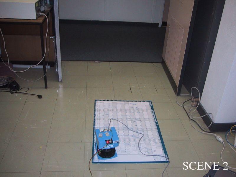
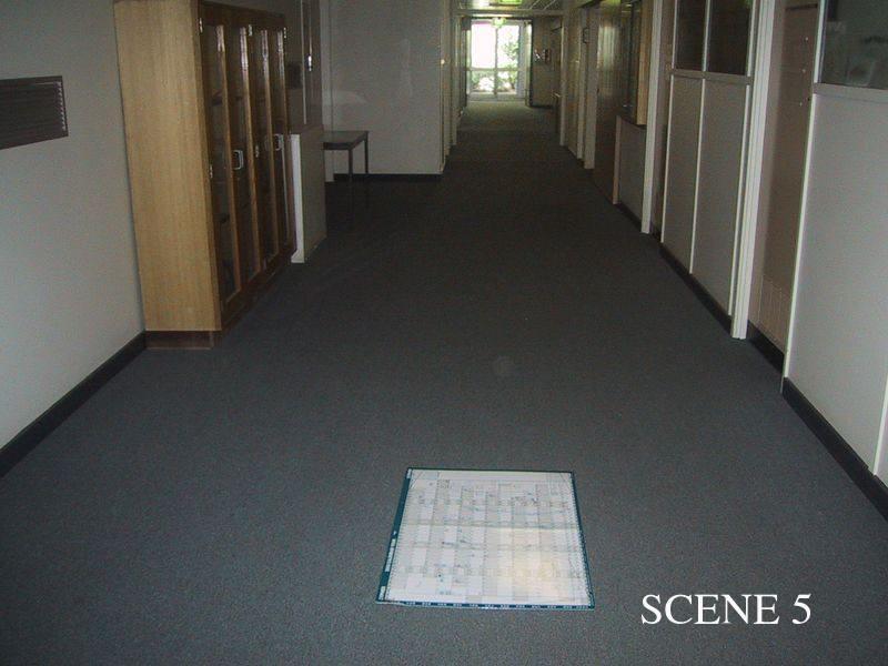
35 6 EXPERIMENTAL RESULTS 34 Figure 18: A photo of each scene with the plastic sheet in the foreground.

36 6 EXPERIMENTAL RESULTS 35 Figure 19: Scan match result for each scene for match number 3 in the experiment with ground truth using PSM.

37 6 EXPERIMENTAL RESULTS 36 Figure 20: Match 3 scan match error evolution for each scene in the experiment with ground truth using PSM. Error in x (circles),y (triangles) and orientation (crosses) are expressed in [cm] and [ ], respectively. Grid size is 1ms x 10cm and 1ms x 10, respectively. Iterations are marked with small vertical lines on the horizontal axis. Each 10-th iteration is marked with a longer vertical line.

38 6 EXPERIMENTAL RESULTS 37 Figure 21: Scan match result for each scene for match number 3 in the experiment with ground truth using PSM-C.

39 6 EXPERIMENTAL RESULTS 38 Figure 22: Match 3 scan match error evolution for each scene in the experiment with ground truth using PSM-C. Error in x (circles),y (triangles) and orientation (crosses) are expressed in [cm] and [ ], respectively. Grid size is 1ms x 10cm and 1ms x 10, respectively. Iterations are marked with small vertical lines on the horizontal axis. Each 10-th iteration is marked with a longer vertical line.

40 6 EXPERIMENTAL RESULTS 39 Figure 23: Scan match result for each scene for match number 3 in the experiment with ground truth using ICP.

41 6 EXPERIMENTAL RESULTS 40 Figure 24: Match 3 scan match error evolution for each scene in the experiment with ground truth using ICP. Error in x (circles),y (triangles) and orientation (crosses) are expressed in [cm] and [ ], respectively. Grid size is 1ms x 10cm and 1ms x 10, respectively. The horizontal resolution of the grid for scene 0 is 10ms. Iterations are marked with small vertical lines on the horizontal axis. Each 10-th iteration is marked with a longer vertical line.

42 6 EXPERIMENTAL RESULTS 41 0 (0.9, 1.5, 0.3) (0.7, 0.4, 1.3) (1.1, 0.2, 0.1) (1.5, 0.4, 2.4) (0.6, 7.4, 0.2) (3.6, 0.1, 1.3) 14, , , , , , (5.1, 17.3, 5.5) (7.7, 13.1, 5.8) (0.4, 24.8, 8.3) (1.0, 1.5, 0.4) (0.3, 5.0, 0.6) (2.4, 0.5, 0.6) 20, , , , , , (0.4, 0.3, 0.3) (0.2, 0.6, 0.1) (0.5, 1.0, 0.3) (0.2, 0.9, 0.3) (0.2, 4.8, 0.3) (1.0, 2.7, 0.3) 8, , , , , , (9.7, 5.0, 0.2) (51.8, 25.3, 0.2) (22.1, 11.1, 0.3) (90.8, 19.4, 0.0) (24.3, 11.2, 0.1) (55.3, 46.3, 0.1) 18, , , , , , ERROR (4.2, 47.9, 1.3) (0.9, 4.3, 0.0) (61.6, 160.3, 4.7) (73.8, 210.5, 1.5) (1.0, 6.1, 0.1) 20, , , , , (0.6, 20.3, 0.4) (0.2, 24.0, 0.4) (1.3, 10.7, 0.4) (12.6, 49.3, 0.5) (3.6, 6.6, 0.9) (1.6, 4.6, 1.5) 24, , , , , , (1.4, 30.7, 0.3) (2.0, 63.0, 0.1) (2.7, 79.1, 0.2) (23.0, 85.2, 0.4) (21.8, 86.6, 0.3) (0.8, 4.7, 0.0) 18, , , , , 3.0 9, (0.2, 0.1, 0.0) (1.5, 0.2, 0.2) (0.1, 0.3, 0.1) (0.8, 2.6, 0.3) (0.9, 4.9, 0.1) (0.0, 0.6, 0.3) 26, , , , , , (0.7, 0.0, 0.0) (1.3, 2.1, 0.1) (0.1, 0.4, 0.3) (0.6, 0.6, 1.9) (0.0, 5.6, 0.9) (0.6, 0.4, 0.1) 11, , , , , , (3.7, 1.7, 0.8) (2.0, 0.4, 0.4) (1.4, 0.9, 0.2) (2.8, 3.0, 0.5) (1.6, 9.5, 0.7) (1.1, 1.6, 0.2) 10, , , , , , 2.4 Table 5: Absolute errors in x[cm], y[cm], θ[ ], number of iterations and runtime [ms] of the PSM algorithm in the experiments with ground truth. 0 (0.7, 1.4, 0.2) (0.8, 0.4, 1.3) (1.0, 0.3, 0.2) (1.6, 0.0, 2.4) (0.8, 6.5, 0.4) (3.0, 0.3, 1.1) 13, , , , , , (7.7, 19.3, 5.4) (7.4, 15.0, 6.2) (1.4, 26.7, 8.5) (1.2, 1.3, 0.3) (4.9, 16.3, 2.8) (1.0, 0.1, 0.4) 12, , , , , , (0.4, 0.1, 0.3) (0.8, 0.5, 0.1) (0.3, 0.7, 0.4) (0.3, 1.0, 0.3) (0.2, 4.6, 0.4) (1.0, 2.5, 0.3) 9, , , , , , (13.2, 6.9, 0.3) (49.4, 24.0, 0.2) (34.1, 17.2, 0.2) (71.5, 14.5, 0.0) (23.2, 10.9, 0.0) (29.1, 24.7, 0.1) 9, 1.5 5, 0.9 6, , 2.8 6, 1.0 9, (2.6, 44.4, 2.5) (6.0, 57.3, 1.6) (0.9, 1.5, 0.0) (53.8, 133.5, 5.3) (65.4, 169.9, 5.8) (6.1, 23.8, 0.2) 17, , , , , , (1.2, 17.8, 0.6) (0.1, 39.7, 0.5) (0.9, 25.8, 0.4) (13.8, 54.6, 0.4) (3.2, 2.8, 1.3) (0.9, 0.5, 0.7) 17, , , , , , (1.3, 24.1, 0.4) (1.5, 58.1, 0.4) (2.7, 74.1, 0.0) (19.6, 71.1, 0.3) (20.3, 79.9, 0.1) (1.3, 4.3, 0.3) 17, , , , , 2.9 9, (0.6, 0.1, 0.1) (0.9, 0.3, 0.1) (0.6, 0.0, 0.1) (1.5, 2.5, 0.3) (1.2, 4.9, 0.2) (0.2, 0.8, 0.1) 17, , , , , , (0.6, 0.7, 0.1) (1.1, 2.0, 0.3) (0.1, 0.3, 0.2) (0.5, 0.1, 2.2) (8.5, 13.3, 6.6) (0.3, 0.1, 0.0) 13, , , , , , (1.5, 1.4, 0.6) (1.5, 1.1, 0.2) (1.3, 2.5, 0.0) (2.3, 2.4, 0.1) (0.2, 5.2, 0.5) (0.8, 1.4, 0.2) 13, , , , , , 2.9 Table 6: Absolute errors in x[cm], y[cm], θ[ ], number of iterations and runtime [ms] of the PSM C algorithm in the experiments with ground truth.

43 6 EXPERIMENTAL RESULTS 42 0 (0.4, 0.1, 0.5) (0.2, 0.5, 1.3) (0.9, 0.2, 0.4) (0.4, 1.5, 4.1) (0.7, 5.3, 0.7) (1.4, 0.8, 1.0) 56, , , , , , (7.2, 16.5, 6.4) (2.1, 1.6, 1.0) (13.0, 29.9, 9.6) (11.0, 88.9, 27.0) (13.5, 53.3, 0.6) (24.7, 5.5, 22.6) 18, , , , , , (0.2, 1.1, 1.3) (0.1, 0.6, 0.4) (1.2, 1.7, 1.8) (0.1, 1.1, 1.6) (1.3, 5.4, 1.1) (2.1, 4.4, 4.6) 25, , , , , , (3.0, 1.3, 0.2) (40.5, 19.9, 0.1) (37.8, 19.6, 0.3) (30.7, 4.5, 0.2) (30.5, 12.8, 0.0) (6.9, 5.7, 0.1) 8, , 9.1 9, , 4.6 8, , (0.5, 2.7, 1.3) (5.5, 61.3, 1.5) (6.2, 55.5, 1.5) (9.4, 54.3, 1.4) (10.7, 70.1, 1.3) (5.8, 22.4, 0.1) 21, , , , , , (0.1, 1.4, 0.1) (7.8, 89.4, 4.3) (0.6, 47.4, 0.4) (15.4, 98.7, 6.3) (14.6, 67.7, 0.0) (0.3, 2.2, 0.1) 35, , , , , , (0.1, 1.4, 0.1) (1.6, 65.4, 0.5) (2.4, 63.7, 0.1) (14.7, 56.7, 1.1) (17.0, 68.6, 0.2) (0.6, 0.5, 0.4) 23, , , , , , (0.2, 0.1, 0.0) (0.4, 0.0, 0.1) (0.1, 0.2, 0.3) (0.5, 3.1, 0.3) (1.6, 6.5, 3.0) (0.0, 0.2, 0.6) 19, , , , , , (1.9, 0.3, 2.0) (0.2, 0.1, 0.5) (28.0, 89.1, 11.6) (45.5, 55.9, 22.6) (2.1, 7.2, 1.9) (0.3, 0.4, 0.7) 28, , , , , , (1.1, 0.8, 0.8) (19.5, 55.6, 11.8) (1.0, 0.4, 0.6) (23.4, 42.0, 28.6) (0.5, 4.8, 0.4) (0.4, 1.8, 1.4) 43, , , , , , 17.7 Table 7: Absolute errors in x[cm], y[cm], θ[ ], number of iterations and runtime [ms] of the ICP algorithm in the experiments with ground truth. 6.4 Convergence Map The purpose of this experiment is to find those initial poses from which scan matching converges to an acceptable solution. Ideally one varies the initial position and orientation of the current scan in a systematic way and observes if the found solution is close enough to the true solution. Areas of convergence can be visualized by drawing the trajectory of the current scan into an image. To make visualization simpler just like in [Dudek and Jenkin, 2000] only the initial pose was changed. Scan pairs from scenes 0-9, match 2 were selected for the convergence map experiment. Match 2 was selected in this experiment because the point of view for the current and reference scan differed the most from all matches. The initial orientation error was always 12. The initial position varied from -250cm to 250cm for x and y in 10cm increments. The resulting convergence plots for scene 9 can be seen in fig. 25. Dark circles represent initial positions where the scan matching algorithms failed for the lack of associated points. Light colored circles represent final positions. Black lines correspond to the trajectories of the scans. Gray crosses mark the correct current scan positions. When examining fig. 25, one has to keep in mind that in all scan matching implementations, associations having a larger error than one meter were discarded. To get an objective value for the performance of the implementations, the total number of matches and the number of successful matches were counted. Successful matches were matches with less than 10cm error in position and 2 in orienta-

44 6 EXPERIMENTAL RESULTS 43 Figure 25: PSM, PSM-C and ICP convergence maps.