ME 261: Numerical Analysis Lecture-12: Numerical Interpolation

Transcription

1 1 ME 261: Numerical Analysis Lecture-12: Numerical Interpolation Md. Tanver Hossain Department of Mechanical Engineering, BUET

2 2 Inverse Interpolation Problem : Given a table of values Find x such that : f ( x) y k, where y k is given x i x 0 x 1. x n y i y0 y1. yn One approach: Use polynomial interpolation to obtain f n (x) to interpolate the data then use Newton s method to find a solution to x f ( x) n y k

3 3 Inverse Interpolation Inverse interpolation: 1. Exchange the roles of x and y. x i y i x 0 x1 y0 y1.. xn yn 2. Perform polynomial Interpolation on the new table. 3. Evaluate yi y0 y1 xi x0 x1.. yn xn x f n ( y k )

4 4 Inverse Interpolation Example x Problem : y Given the table. Find x such that f ( x) x x f f 2 2 ( y) ( y 3.2) ( y 3.2)( y 2) (2.5) ( 0.7) ( 0.7)(0.5)

5 5 Why Spline Interpolation? Apply lower-order polynomials to subsets of data points. Spline provides a superior approximation of the behavior of functions that have local, abrupt changes.

6 6 Why Splines? 17 th Order Polynomial Original Function 5 th Order Polynomial 9 th Order Polynomial Figure : Higher order polynomial interpolation is a bad idea

7 7 Spline Interpolation Polynomials are the most common choice of interpolants. There are cases where polynomials can lead to erroneous results because of round off error and overshoot. Alternative approach is to apply lower-order polynomials to subsets of data points. Such connecting polynomials are called spline functions.

8 Spline provides a superior approximation of the behavior of functions that have local, abrupt changes (d). 8

9 Spline Interpolation The concept of spline is using a thin, flexible strip (called a spline) to draw smooth curves through a set of points.natural spline (cubic) 9

10 10

11 11 Linear Spline The first order splines for a group of ordered data points can be defined as a set of linear functions: f ( x)= f ( x 0 )+m 0 ( x x 0 ) x 0 x x 1 f ( x)= f ( x 1 )+m 1 ( x x 1 ) x 1 x x 2 f ( x)= f ( x n 1 )+m n 1 ( x x n 1 ) x n 1 x x n m i = f ( x i+1 ) f ( x i ) x i+1 x i

12 Linear spline - Example 12 Fit the following data with first order splines. Evaluate the function at x = 5. x f(x) m= = 0.6 f (5)= f (4.5)+m(5 4.5) = = 1.3

13 Linear Spline 13 The main disadvantage of linear spline is that they are not smooth. The data points where 2 splines meets called (a knot), the changes abruptly. The first derivative of the function is discontinuous at these points. Using higher order polynomial splines ensure smoothness at the knots by equating derivatives at these points.

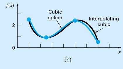
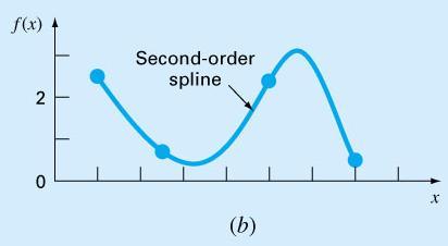
14 Quadric Splines 14 Objective: to derive a second order polynomial for each interval between data points. f i ( x )= a i x 2 +b i x+c i Terms: Interior knots and end points For n+1 data points: i = (0, 1, 2, n), n intervals, 3n unknown constants (a s, b s and c s)

15 Quadric Splines 15 The function values of adjacent polynomial must be equal at the interior knots 2(n-1). a i 1 x 2 +b i 1 x i 1 +c i 1 = f i ( x i 1 ) i= 2, 3, 4,..., n i 1 a i x i 1 2+b i x i 1 +c i = f i ( x i 1 ) i= 2, 3, 4,..., n The first and last functions must pass through the end points (2). a 1 x 0 2 +b 1 x 0 +c 1 = f ( x 0 ) a n x n 2+b n x n +c n = f ( x n )

16 Quadric Splines 16 The first derivatives at the interior knots must be equal (n-1). f i ' ( x)= 2a i x+b i 2a i 1 x i 1 +b i 1 = 2a i x i 1 +b i Assume that the second derivate is zero at the first point (1) a 1= 0 (The first two points will be connected by a straight line)

17 Quadric Splines - Example 17 Fit the following data with quadratic splines. Estimate the value at x = 5. Solutions: There are 3 intervals (n=3), 9 unknowns.

18 Quadric Splines - Example Equal interior points: For first interior point (4.5, 1.0) For second interior point (7.0, 2.5)

19 19 Quadric Splines - Example First and last functions pass the end points For the start point (3.0, 2.5) x 2 0 a 1 +x 0 b 1 +c 1 = f ( x 0 ) 9a 1 +3b 1 +c 1 = 2.5 For the end point (9, 0.5) x 2 3 a 1 +x 3 b 3 +c 3 = f ( x 3 ) 81a 3 +9b 3 +c 3 = 0.5

20 20 Quadric Splines - Example Equal derivatives at the interior knots. For first interior point (4.5, 1.0) For second interior point (7.0, 2.5)

21 21

22 22 Quadric Splines - Example Solving these 9 equations with 9 unknowns a 1 = 0, b 1 = 1, c 1 = 5.5 a 2 = 0.64, b 2 = 6. 76, c 2 = a 3 = 1. 6, b 3 = 24. 6, c 3 = f 1 ( x)= x+5.5, 3.0 x 4.5 f 2 ( x)= x x+18.46, 4.5 x 7.0 f 3 ( x)= 1.6x x 91.3, 7.0 x 9.0

23 23 Cubic Splines Objective: to derive a third order polynomial for each interval between data points. Terms: Interior knots and end points f i ( x )= a i x 3 +b i x 2 +c i x+d i For n+1 data points: i = (0, 1, 2, n), n intervals, 4n unknown constants (a s, b s,c s and d s)

24 Cubic Splines 24 The function values must be equal at the interior knots (2n-2). The first and last functions must pass through the end points (2). The first derivatives at the interior knots must be equal (n-1). The second derivatives at the interior knots must be equal (n-1). The second derivatives at the end knots are zero (2), (the 2 nd derivative function becomes a straight line at the end points)