A Shape-Independent-Method for Pedestrian Detection with Far-Infrared-Images

Transcription

1 A Shape-Independent-Method for Pedestrian Detection with Far-Infrared-Images Yajun Fang +, Keiichi Yamada +, Yoshiki Ninomiya*, Berthold Horn +, Ichiro Masaki + + Intelligent Transportation Research Center, Microsystems Technology Labs Massachusetts Institute of Technology, Cambridge, MA 2139, USA Toyota Central R &D Labs, Inc. Japan yjfang@mit.edu, yamakei@mit.edu, nino@milab.tytlabs.co.jp, bkph@ai.mit.edu, masaki@mit.edu Abstract Night-time driving is more dangerous than day-time driving particularly for older drivers. Three to four times as many deaths occur at night than in the day time [1]. To improve safety of night driving, automatic pedestrian detection based on infrared images has drawn increasing attention because pedestrians tend to stand out more against the background in infrared images than they do in visible light images. Nevertheless, pedestrian detection is by no means trivial in infrared images many of the known difficulties carry over from visible light images, such as image variability occasioned by pedestrians being in different poses. Typically, several different pedestrian templates have to be used in order to deal with a range of poses. Furthermore, pedestrian detection is difficult because of poor infrared image quality (low resolution, low contrast, few distinguishable feature points, little texture information, etc.) and misleading signals To address these problems, this paper introduces a shape-independent pedestrian detection method. Our segmentation algorithm first estimates pedestrians horizontal locations through Projection-based horizontal segmentation, and then determines pedestrians vertical locations through Brightness/Bodyline-based vertical segmentation. Our classification method defines multi-dimensional histogram-, inertial-, and contrast-based classification features, which are shape-independent, complementary to one another, and capture the statistical similarities of image patches containing pedestrians with different poses. Thus, our pedestrian detection system needs only one pedestrian template corresponding to a generic walking pose and avoids brute-force search for pedestrians throughout whole images, which typically involves brightness-similarity-comparisons between candidate image patches and a multiplicity of pedestrian templates. Our pedestrian detection system is not based on tracking, nor does it depend on camera calibration to determine the relationship between an object s height and its vertical image locations. Thus, it is less restricted in applicability. Even if much work is still needed to bridge the gap between present pedestrian detection performance and the high reliability required for real-world applications, our pedestrian detection system is straightforward and provides encouraging results in improving speed, reliability, and simplicity. I. Introduction Automatic detection of pedestrians at night has attracted more and more attention. Eighty percent of police reports [8] cited driver errors as the primary cause of vehicle crashes. Because depth perception, color recognition, and peripheral vision are all impaired after sundown, 3 4 times as many deaths occur during night-time driving than day-time driving. Also, people s visual capabilities deteriorate substantially as they age, as is shown in figure 1, which compares the visual ability of a driver of age 6 with those of a driver of age 2. A 5-year-old driver needs twice as much light to see as does a 3-year-old [1]. Fig. 1. Vision Degradation for Senior People. (Image Source: MIT Age Lab.) To enhance safety, current night vision systems use infrared-cameras to provide visual aids projected on a heads-up display. In the long run, however, automatic pedestrian detection and warning is envisioned so that drivers can respond promptly without being distracted by added gadgetry. Compared to the vast research on pedestrian detection based on visible light images [2][3][5][14][16][19] as summarized in [11][12][18], work on infrared-based pedestrian detection research [11][12][18] has just started. In an earlier paper [6], we systematically compared different properties of visible and infrared images and noted several unique features of infrared-based pedestrian detection. In this paper, we further investigate the statistical properties of these features and introduce a novel shape-independent pedestrian detection scheme including automatic pedestrian image size estimation and multi-dimensional shape-independent classification. In

2 this section, we first discuss how we evaluate detection performance, then review previous work and analyze challenges associated with automatic pedestrian detection using infrared images. Finally we will discuss the advantages of our design as well as differences from conventional methods. A. Performance Index Pedestrian detection [5] [14] includes two phases: segmentation locates multiple regions of interest (ROIs) from infrared images, and classification identifies pedestrians from the ROIs. In this paper, we evaluate both segmentation and classification performance. For segmentation, we define two new performance indices: segmentation side-accuracy and segmentation side-efficiency as shown in figure 2(a). Segmentation side-accuracy is defined as the square root of ratio of the detected pedestrian region area S overlap over the entire pedestrian area S pedestrian, which indicates how much of the pedestrian regions are captured. If, for example, the segmentation side-accuracy is 5%, then the width and height of the detected region might be only half of the actual pedestrian s width and height. Segmentation side-efficiency is defined as the square root of the ratio of the detected pedestrian area S overlap over the entire ROI area S ROI, which indicates how efficient the selection of the ROI regions is. If, for example, the segmentation side-efficiency is 5%, then the width and height of the detected pedestrian region might be only half of the actual ROI s width and height. Both performance measures lie in the range [, 1]. The best segmentation performance is achieved when both measures are 1, which means that ROIs and actual pedestrian regions overlap completely. High segmentation accuracy with low efficiency indicates that, while most pedestrian regions are detected, this is at the cost of a large unnecessary ROI area. Conversely, low segmentation accuracy with high efficiency indicates that the ROIs capture only a small portion of the pedestrians, though most ROI regions are within pedestrian regions. (a) (b) Fig. 2. Segmentation/Classification Performance Index Definition. (a): Segmentation Accuracy/Efficiency definition. (b): ROC boundary/curve definition for multi-dimensional-feature based classification: false alarm rate (X axis) vs. detection rate (Y axis). Different points correspond to multi-dimensional-feature-based classification results using different multi-dimensional thresholds. Solid curve is ROC boundary, the upper/left boundary of all classification performance points. Dashed and dotted curves are ROC curves for 1D-feature-based classification. To evaluate classification performance for multi-dimensional-feature-based classification, we use different multi-dimensional thresholds, and plot corresponding false-alarm/detection rates as points in a 2D performance space (X axis: false alarm rate/y axis: detection rate) as shown in figure 2(b). Classification performance improves when a performance point moves toward the upper and left direction. Obviously the best performance is at the upper/left corner with 1% detection rate and % false-alarm rate. However, if one point is to the upper and right of another point, we cannot easily compare their performance. The upper/left boundary of classification performance points, as shown in solid curves in figure 2(b), can be used to demonstrate the classification ability of an algorithm, and is called the ROC (Receiver Operating Characteristics) boundary in this paper. The ROC boundary for 1D based classification degrades to the conventional ROC curve as shown by the dotted and dashed curves in figure 2(b). The ideal ROC curve/boundary is approximately a vertically flipped L shape as shown in figure 2(b). All ROC curves/boundaries include two points, (, ) and (1%, 1%), which can be achieved by rejecting all or accepting all. In this paper, detection/false-alarm rates on the ROC curves are shown for ROIs (rather than image frames). We also calculate frame detection/false-alarm rate for performance comparison with other published results. To calculate the number of detected frames, we count frames in which all pedestrians are detected, and empty frames (with no pedestrian) in which there is no false alarm. However we do not plot an ROC curve for frame detection/false-alarm rates since it also depends on segmentation performance and consequently does not necessarily pass through the (1%, 1%) detection/false-alarm rate point, which is different from typical ROC curves. 2

3 B. Challenges and Reviews for Pedestrian Detection with Infrared Images Pedestrian detection using infrared images has its own advantages as well as disadvantages [6][11][12][18] when compared with detection using visible light images. In general, pedestrians emit more heat than static background objects, such as trees, roads, etc. In far-infrared images, pedestrian brightness tends to be less impacted by lighting, color, texture, and shadow information than it is in visible light imagery, and is generally also somewhat brighter than the background. However, infrared image intensities depend not only on object temperature but also on object surface properties (emissivity, reflectivity, and transmissivity), surface orientation, wavelength, etc. Infrared images have their own characteristics that lead to detection difficulties. First, non-pedestrian objects, such as, animals, vehicles, transformers, electric boxes, roads, construction areas, light poles, etc., produce additional bright areas in infrared images, especially in summer. These additional sources of image clutter make it impossible to reliably detect pedestrians based only on their brightness. Secondly, the image intensities of the same objects are not uniform. Pedestrian orientation, clothes, accessories (such as backpacks), etc., all have an impact on observed image intensity patterns. Body-trunk areas are generally darker than head and hand areas, especially when pedestrians wear heavy coats or carry backpacks. The upper parts of light poles appear brighter than the lower parts because of contrast phenomena in typical far-infrared cameras. Non-homogeneous optical properties add to detection difficulties. Thirdly, most infrared image intensities have a smaller intensity range than do comparable visible images. This leads to low image quality: blur, poor resolution and clarity, low foreground/background contrast, fewer feature points and less texture information, etc. Thus, current infrared-based pedestrian detection research is still limited [6][7][11][12][16][18]. Both segmentation accuracy and classification reliability of early night vision research needs to be significantly improved for it to be used practically [18][12]. For example in winter, to have a false-alarm rate around 2.63% [18], the detection rate has to be limited to only 35%. In summer, to have 75% to 9% detection rate, the false-alarm rate has to be raised to 1% [12] as shown in figure 3(a). Below we will discuss inherent difficulties in two phases and then review related current work. (a) (b) (c) Fig. 3. Algorithm and Performance Comparison for Different Pedestrian Detection Methods. (a): Detection Performance Comparison. (b): Detection Algorithm Comparison. (c): Default Pedestrian Template for MIT Shape-Independent Method. Image size: B.1 Challenges and Reviews for ROI Segmentation It is difficult to segment pedestrians in real-world video images captured by moving-cameras mounted on vehicles. Pedestrians have a variety of poses, sizes and appearances, and the background is changing rapidly as the cameras move through the environment. Many conventional fast segmentation algorithms have been developed for stationary cameras, such as Background Subtraction [15], Motion Calculation, and Tracking. These methods assume similar background or feature points, and need initialization time. Thus it is expected that pedestrian detection for intelligent vehicles can rely only on single static image instead of multiple-image-based (motion-based) algorithms. Conventionally, segmentation based on depth information is more straightforward than other methods and multi-scale brute force searching can be avoided. However binocular-infrared-camera-setup is not widely used in most night vision research, except by Tsuji (21) [16]. There might be reliability concern because of the properties of infrared images discussed above and nodding movement of cameras on vehicles [6]. If detailed pedestrian contours can be extracted, pedestrians can be identified by using Contour-based Shape Model [2][3][5], such as, pedestrian shapes hierarchy[5] or 3

4 human walking model[3]. Besides, Human Component Features [4][5][1][13][17], such as skin hue, eyes, faces, etc., also help when segmenting pedestrians in visible images. The above well known fast segmentation features are non-applicable to far-infrared images because of their unique properties. It is also hard to segment pedestrians by grouping bright spots belonging to pedestrians based only on their pixel intensities. Using one fixed brightness threshold, for example, will lead to several separated bright spots at both pedestrian regions and other noise resources, with results highly sensitive to the choice of brightness thresholds. If introducing Template-Shape-based multi-scale brute-force searching as some night vision algorithms do (as shown in Figure 3(b)), segmentation ROI outputs are all candidate pedestrian patches of different sizes and aspect ratios, at multiple initial locations. The total number of ROIs for completely blind multi-scale brute force searching is as follows: n ROI = n scale i=i n i center pos n row n column n scale (1) where n scale is the number of scales in estimating pedestrian sizes, n i center pos is proportional to the image size ( n row n column ), which is the number of initial ROI center positions that must be tried when testing at different scales. The large search space for blind searching is a serious limitation in Different segmentation algorithms take advantage of different features to decrease n ROI and to expedite the searching process. To decrease n center pos, [18] searches bright and round regions as potential pedestrian heads in infrared images. [11] searches hot symmetrical ROIs with specific size and aspect ratio based on the Symmetry Property of pedestrians and their brightness[9]. To decrease n scale, [18] and [11] assume flat roads so that pedestrians distance can be estimated based on pedestrians vertical positions in images. [18] first detects road surface boundaries in order to estimate pedestrians sizes and height and remove impossible pedestrian size/position combinations. [11] calibrates infrared cameras to build correspondences between image lines and distances in the 3D world for pedestrian size estimation. [12] does not make any assumptions and searches only three pedestrian sizes in a multi-scale brute force approach. The segmentation accuracy is limited compared with [11][18]. For real-world applications, segmentation algorithms need to further improve speed and accuracy and make fewer assumptions on the driving environment. B.2 Challenges and Review for Classification In far-infrared images, pedestrians yield widely varying image patterns because of the imaging complexity mentioned before and variations in pedestrian poses. When presented with multiple candidate image regions, differentiating pedestrians from non-pedestrian regions is difficult. Typically the decision is made based on the similarity between ROI regions and multiple pedestrian templates with various poses and appearances. Similarity can be computed either directly or indirectly. Typical direct methods compare image intensity pixel-by-pixel and compute the Image-Intensity-Difference between two patches, i.e., the Frobenius norm of image pixel intensity differences. The classification methods heavily depend on shape matching and as a result are sensitive to segmentation errors and variations in pedestrian poses. [12] defines a template probabilistic model to encodes the shape information of pedestrians and the variations that the shape can undergo by describing the possibility of foreground and background at each pixel based on training data. [11] identifies pedestrians through matching candidates with a simple model that encodes morphological characteristics of a pedestrian. The shape-dependent filter removes candidates that do not present a human shape or are not as hot as expected for a pedestrian. For indirect similarity-comparison, shape-dependent pedestrian-intensity-arrays are used to train classifiers to capture the similarity between pedestrian training samples and ROIs, for example, support Vector Machine [14] [18], Neural Network [13][19], Posteriori Detection (including Polynomial Classifiers, Multi-Layer Perceptrons, and Radial-basis Functions), etc., (as shown in figure 3(b)). [18] proposed SVM (support vector machine) classifiers for three types of pedestrians for infrared images. These brightness-similarity-comparison based classification methods are shape-dependent, and might miss pedestrians with unusual poses even if multiple pedestrian-pose-templates or training samples are used. Furthermore, complicated machine-learning methods require significant computational resources. In summary, speed, reliability, and performance robustness to pose-changes and segmentation errors are serious concerns for real-world night vision systems. C. The Methodology and Principle for Shape-Independent Pedestrian Detection Because of the above mentioned difficulties involved in shape dependent and/or brute-force searching based methods, the performance of present pedestrian detection systems is limited as shown in figure 3(a). In this paper, we introduce a Shape-Independent automatic pedestrian detection method with straightforward implementation. Figure 3(b) presents the major differences between our shape-independent methods and conventional shape-dependent methods. The algorithm can automatically estimate the horizontal location of candidate pedestrian regions to avoid brute-force multiscale searching. Our novel classification feature vectors can characterize the statistical similarity of multiple pedestrian regions with different poses, and can also capture the statistical differences between pedestrian and non-pedestrians regions in infrared images. Thus, our multi-dimensional classification needs only one generic pedestrian template as 4

5 shown in figure 3(c) with size (details in section III). The method is based on the unique statistical properties of far-infrared images that we discovered through investigating the differences between visible and infrared images [6]. Our method has the following properties. First, it focuses on improving combined segmentation/classification systems and balances the complexity and performance of two subsystems instead of maximizing one process while sacrificing the other. This is because accurate segmentation can ease the classification task and robust classification can tolerate segmentation errors. Secondly, our segmentation procedure is robust to threshold choices. Finally, our algorithm does not make constraining assumptions for background, for example that flat roads; thus our results are very general. The classification performance comparison is shown in figure 3(a). For pedestrian detection in winter, we achieve a higher detection rate when we set the false alarm rate to be similar to other available published results. For summer, we achieve a lower false alarm rate when we set the detection rate to be similar to other available published results. In the rest of the paper, we will introduce our Automatic Pedestrian Segmentation, and Shape-Independent Multiple Dimensional Classification respectively in section II and III. Performance evaluation and future work will be discussed in section IV and section V. II. Automatic Pedestrian Segmentation As mentioned in I-B.1, conventional Template-Shape-based segmentation involves searching with computational load Ø(n 2 ). We invented a new horizontal-first, vertical-second segmentation scheme involving only 1D searching in vertical direction with computational load Ø(n). The method first automatically estimates the horizontal locations of candidate pedestrian regions, and then searches for pedestrians images vertically within the corresponding image stripes (from top to bottom in the images) at the estimated horizontal positions. Thus search space and computational load are reduced significantly. In this section, we will respectively introduce our horizontal segmentation algorithm based on bright-pixel-vertical-projection curves, and vertical segmentation based on brightness/bodylines. A. Horizontal Segmentation Here below we will first define the bright-pixel-vertical-projection curve, then explain how and why we can use this concept to estimate pedestrians horizontal locations. A.1 Bright-pixel-vertical-projection Curves For an infrared image, we define its bright-pixel-vertical-projection curves as the number of bright pixels in image columns versus their corresponding horizontal positions. To count Bright Pixels, the intensity threshold is adaptively defined as follows: Bright Pixel Threshold =max(image Intensity) - Intensity Margin (2) where the variable Intensity Margin is a fixed constant for different video sequences. Typically the bright-pixelvertical-projection curves can be divided into several bumps or waves with rising left curves and falling right curves, as well as flat regions with zero height whose corresponding image stripes have no bright pixel as shown in figure 4(b). Each pedestrian image will be captured in one image stripe corresponding to one such wave. In most cases the width of the pedestrian-image-region is equal to the width of the corresponding wave as shown in figure 4(a)(b). The features of the defined curve is robust to the choices of brightness threshold and problems mentioned in section I- B. Figure 4(a) shows the variation of projection curves corresponding to two different brightness thresholds. Generally, the height and shape of the waves in the curves will change. However the horizontal locations and width of waves corresponding to pedestrians will not change significantly. This is because of the following two reasons: First, for typical real-world far-infrared images, the image stripe containing one pedestrian is narrow and the number of bright background pixels in each column can be treated as more or less constant unless there happens to be some light poles, for example, which may tend to also appear narrow and bright, at least in summer. Later we will discuss how pedestrians can be detected in this special case. Secondly, image columns passing through pedestrian regions tend to encounter more bright pixels than neighbor columns passing background regions. Both of these features are independent of the choices of brightness thresholds. A.2 Projection-based Horizontal Segmentation Algorithm Based on the above properties of the bright-pixel-vertical-projection curves, we can segment an image horizontally into several image stripes (as shown in the bottom row of figure 4(b)), some of which contain individual pedestrians and roughly determine candidate pedestrians image width. The procedure is as follows: 1. Adaptively choose an brightness threshold using equation (2). Record the number of bright pixels in each column in the bright-pixel-vertical-projection curves. We select a large constant Intensity Margin in equation (2) that 5

6 (a) (b) (c) (d) Fig. 4. The Feature of Bright-Pixel-Vertical-Projection Curves for Infrared Images and Brightness-based Vertical Segmentation Results. For (a)(c): Winter results. For (b)(d): Summer results. (a): Top row: original infrared image in winter. Center row and Bottom row: Bright-Pixel-Vertical-Projection curves when using two different thresholds. (b): Top row: original infrared image in summer. Center row: Bright-Pixel-Vertical-Projection Curve. Bottom row: Horizontally segmented image stripes based on projection curve. Note that Several separated stripes shown in the center row seem to be connected. For (c)(d): Brightness-based vertical segmentation results. For all projection curves: X axis: Image column position. Y axis: Number of bright pixels in each column. makes the brightness threshold adaptively small to ensure that the image columns containing pedestrians will have non-zero projection in the bright-pixel-vertical-projection curves. 2. Automatically search for the starting points of all rising curves (wave-start-points) and the ending points of all falling curves (wave-end-points). 3. Separate the bright-pixel-vertical-projection curves into several waves by pairing wave-start-points and wave-endpoints, and ignoring flat regions of zero height. 4. Record image stripes corresponding to these waves. Because of background brightness noises in summer, projection curves for winter and summer images, as shown in figure 4(a)(b), have the following different properties. First, in winter, waves corresponding to pedestrians usually have higher peaks than background waves, unlike summer where background noises may produce high wave peaks in projection curves as shown in figure 4(b). Secondly, under complicated urban driving scenario in summer, as shown in figure 4(b), pedestrians and background brightness noises may be spatially proximate and their projection thus may merge into one wave, which is the case for the second pedestrian from the left in figure 4(d). For winter images (example: sequence 1 shown in figure 17(a1)) and summer sequences in suburban area (example: sequence 2 in figure 17(b1)) with sparse foreground objects, pedestrian regions are less likely to be grouped with other hot foreground regions. In spite of the differences that might make image stripes wider than the actual pedestrian image width in some cases, pedestrians will be fully captured in individual horizontally separated stripes. So far, we have presented a novel projection-based pedestrian pre-segmentation algorithm that horizontally separates infrared images into several image stripes that may contain pedestrians. In the next section, we will introduce how to 6

7 search pedestrians vertical location in segmented image stripes. B. Vertical Segmentation within Horizontally Segmented Image Stripes Here we will introduce two vertical segmentation algorithms. The first is a Brightness-based method (section II-B.1) that works best in winter and suburban situations where most segmented image stripes for pedestrians reflect the true width of pedestrian-image-regions. The second is a Bodyline-based method (section II-B.2) for more complicated scenarios where the image stripes containing pedestrians might be wider than the pedestrian images true width. These two methods provide complementary results that work best in different scenarios, and the results from both methods are sent to classification step to further improve reliability and accuracy. B.1 Vertical Segmentation based on Brightness After obtaining horizontally segmented image stripes from section II-A.2, the vertical positions of candidate pedestrian regions can be estimated by the highest and the lowest vertical locations of bright pixels within these stripes. This method is applicable when the estimate of the pedestrian region width is reasonably accurate. In this case, most brightness-based vertical segmentation results for both winter and summer data turn out correctly as shown in figure 4(c)(d). Our classification algorithm has the ability to tolerate segmentation errors for pedestrian ROIs, such as the inclusion of extra background regions or conversely missed portion, as shown in the first and the fourth pedestrians from the left in figure 4(c). Non-pedestrian ROIs have bright pixels at the boundaries, which facilitates the inertialbased classification algorithm to be described later in section III-B. When segmentation stripes are much wider than the actual pedestrian image size, ROIs may be much larger than the true width, as occurs for the third pedestrian from the right in figure 4(d). A Bodyline-based vertical segmentation algorithm (explained below) is proposed to improve segmentation performance in such more difficult situations. B.2 Vertical Segmentation based on Bodyline In this method, we refine the pedestrian width estimation by detecting pedestrian regions left and right boundary points within segmented image stripes. Thus we can further search for pedestrians vertical positions based on a geometric pedestrian-size-model as described next. For each row of image stripes, we define the portion of image rows within pedestrian regions as the pedestrianbodyline, and define prominent feature points where image rows meet pedestrian boundaries as pedestrian-bodylineterminals. Figure 5(a) presents one bodyline example in the waist area of a pedestrian image. Below we will describe in detail how to detect bodyline, and how to vertically segment pedestrians within image stripes. Step 1 Pedestrian Horizontal Bodyline Detection. Because of infrared image features, in each row within segmented image stripes, the left pedestrian-bodylineterminals are the points where image intensities change from darkness to brightness most rapidly. Similarly, at the right pedestrian-bodyline-terminals, image intensities change from brightness to darkness most rapidly. To obtain pedestrian-bodyline-terminals, we calculate intensity variation along the horizontal direction based on the modified Sobel method as below: I(x, y) = [I(x + 1, y + 1) I(x 1, y + 1) + 2I(x + 1, y) 2I(x 1, y) + I(x + 1, y 1) I(x 1, y 1)]/6 (3) where (x, y) are pixel coordinates, I(x, y) is image intensity, and I(x, y) is pixel-horizontal-spacing. We first calculate pixel-horizontal-spacing for all pixels in each row within horizontal segmentation stripes. Then we search in the left half portion of the row for a point with the largest pixel-horizontal-spacing as the candidate for the left bodyline terminal points. We skip the row where pixel-horizontal-spacing for all pixels is smaller or equal to zero. Similarly, we determine the right bodyline terminal with the most negative pixel-horizontal-spacing in the right half portion of the row. Thus we obtain two outmost boundaries and a bodyline for candidate pedestrians in each row within horizontal segmentation stripes. For segmented image stripes shown in figure 4(b), figure 5(b) preserves all pixels within detected candidate bodylines, in which pedestrians stand out and the background pixels surrounding the pedestrian regions has been removed. It may happen that some boundary points belong to other hot objects next to the pedestrians, and we might not obtain a clear bodyline at every row of pedestrian regions. However, as long as we can obtain one bodyline, in the next step we can still estimate the candidate pedestrian s image size based on the bodyline length. Step 2 Pedestrian Location Estimation based on Pedestrian-Bodyline Matching In figure 5(a), we propose a geometric pedestrian-size-model that defines one pedestrian s size and location based on the location and length of a waist-bodyline. The reason we use waist-bodylines is because the contrast between 7

8 human hip areas and their local background neighborhoods tend to be robust to the poses of walking pedestrians. Horizontal waist-bodylines are more likely to be detected and are not easily missed under a variety of conditions. Using the model, we can define multiple candidate pedestrian regions by assuming each detected bodyline to be the waist-bodyline of an pedestrian. Figure 5(c) provides an example of bodyline-based pedestrian location estimation. A few estimated candidate pedestrian regions are marked. Step 3 Histogram-based Bodyline/Pedestrian Searching Among multiple candidate regions defined previously within a vertical image stripe, there is at most one actual pedestrian image region. Choosing one candidate pedestrian region is essentially a classification problem. We first use one histogram-based classification feature to search for the best candidate within each image stripe. After obtaining one candidate for each image stripe, we further determine whether it is a actual pedestrian image using multi-dimensional classification features explained in the next section. Details of the histogram-based feature and other classification features will be explained in section III. It is worth mentioning that we do not need to use a threshold in the searching process since we choose ROIs that are closest to our default pedestrian template (figure 3(c)) in histogram feature space. (a) (b) (c) (d) Fig. 5. Pedestrian segmentation based on two different methods. (a): Bodyline based geometric pedestrian-size-model. (b): Bodyline image. (c): Candidate pedestrian region estimation based on (a) and (b). (d): Bodyline-based segmentation result. For initial horizontally segmented image stripes in the bottom row of figure 4(b), the bodyline-based vertical segmentation result is shown in figure 5(d), which provide more accurate segmentation results than the brightness-based segmentation results shown in figure 4(d) where background noise causes segmentation errors. In sum, the flowchart of automatic pedestrian segmentation starts with projection-based horizontal segmentation as shown in figure 3(b). Within segmented image stripes, brightness-based vertical segmentation assumes that pedestrian pixels are brighter than the rest of background pixels in the image stripes. The bodyline-based method assumes there exists clear brightness contrast between pedestrian image regions and their horizontal-neighbor-regions, and search for the left-positive/right-negative vertical-edge-pairs with high pixel-horizontal-spacing in order to detect potential pedestrian bodylines and estimate candidate pedestrian positions. Both methods automatically estimate pedestrians sizes and avoid multi-scale brute force searching. The first method is straightforward and works reliably in suburban summer cases as well as winter cases. The second method works in complicated urban driving situations. Neither method needs to assume flat roads and both can work in a general driving situation. In real-world applications, both segmentation results will be fused in classification. Conventional segmentation involves brute force searching within an entire image and produces multiple initial ROIs as in equation (1). Instead, bodyline-based segmentation involves only searching among multiple bodylines within horizontally segmented image stripes and the number of produced initial ROIs is as follows: n bodyline ROI n image stripe n bodyline (4) where n image stripe is the number of horizontally segmented image stripes and is usually less than 2 (even less than the number of image columns), and n bodyline is the largest number of bodylines in segmented image stripes and is much less than the number of image rows. Thus n bodyline ROI is significantly less than in equation (1). The number of ROIs for brightness-based segmentation is equal to n image stripe. In sum, our vertical segmentation produces fewer candidate ROIs. III. Classification To recognize pedestrians, conventional classification is based on brightness-similarity-comparisons between ROIs and multiple templates, which is shape-dependent and is subject to segmentation errors and pose-changes as mentioned in 8

9 section I-B.2. For robustness and reliability, we propose innovative classification that is based on comparing the similarity between multi-dimensional shape-independent feature vectors for ROIs and for one generic pedestrian template. In this section we first introduce histogram-, inertial-, and contrast-based classification features individually, then we will propose our multi-dimensional classification methods and compare the classification ability of our defined shapeindependent features with conventional shape-dependent features. A. Histogram-based Classification In this section we discuss the brightness histogram similarities among pedestrian regions with various poses, sizes and appearances, and introduce the histogram-feature s ability to separate pedestrian/non-pedestrian ROIs based on one generic pedestrian template. A.1 Statistical Similarity of Brightness Histograms for Pedestrian ROIs In section I-B, we have mentioned that pedestrian regions in infrared images are complex and not homogeneous. However, when pedestrians change poses, the intensity patterns should be consistent for similar body areas in different infrared images. Because of similar body temperatures and similar pedestrian surface properties, this observation applies not only for the same pedestrian of different poses, but also for different pedestrians with different gender, clothing, and in different seasons. Thus, there exists the similarity among image-brightness-histogram-curves for pedestrian patches containing different people, with different poses, and in different seasons. This property is demonstrated in histogram curve comparison in figure 6. Figure 6(a) is our default pedestrian template cut from a summer sequence. Figure 6(a1) shows seven pedestrian ROIs from four winter images, in which pedestrians have different poses and are of different gender. Figure 6(b1) demonstrates the similarity among the brightness-histogram-curves for the seven pedestrian regions. Figure 6(c1) compares the average brightness-histogram-curves of the above seven pedestrian regions from winter images(solid line) with the histogram curve for the pedestrian template from summer images(dashed line) in figure 6(a). We further demonstrate statistical histogram similarity for pedestrian regions through the variation of brightnesshistogram-curves from 911 rectangular pedestrian regions in seven different driving sequences. Figure 7(a) shows the examples of pedestrian appearances and sizes in two sample sequences. We normalize all pedestrian patches to a standard size [58 21] (1218 pixels) before calculating their smoothed brightness-histogram-curves, i.e., hist m ROI (i), which is the number of pixels with brightness i. Figure 7(b) defines the histogram variation curve, i.e., the distribution of histogram variation value h m (i) h n (i) for all brightness i. In this way, the variation of all 911 histogram curves hist m ROI from their average histogram hist mean is presented as the collective histogram variation curve in figure 7(c), which resembles a Gaussian shape (of zero mean) with certain skewness. We can see that most histogram shape variation is within [-1, 1] pixels, which is only 8.2% of the largest variation (1218 pixels). The fact provides us statistical evidence that histogram curves for pedestrian regions are very similar. A.2 The Classification Ability of Histogram Feature Figure 6(b2) shows the comparison among all histogram curves for non-pedestrian ROIs in figure 6(a2), and figure 6(c2) shows the comparison between their average and the brightness histogram of a summer pedestrian template, as shown in figure 6(a). The results are drawn with the same scale as figure 6(b1)(c1) with similar comparisons for pedestrian ROIs. The comparison between figure 6 (b) and (c) reveals that histogram features for pedestrian/non-pedestrian ROIs are different in most cases. Because of the histogram similarity for pedestrian regions, as well as histogram differences between pedestrian ROIs and non-pedestrian ROIs, pedestrians can be identified through histogram-similarity-comparison between ROIs and one generic pedestrian template. Without losing generality, we choose figure 6(a) as our generic pedestrian template. The Histogram Difference index is defined as the weighted summation for the square of brightness histogram difference at each brightness i as below: Histogram Difference = α 255 i=1 weight(i) [hist ROI(i) hist template (i)] 2 (5) where hist ROI and hist template are histogram curves for ROIs and a template respectively, α is normalization coefficient, weight(i) is weighting function that is fixed for all classification calculations. Typically segmentation errors might introduce extra dark background or bright regions, leading to higher histogram curve peaks at small/large brightness value. W eight(i) is set to be small when brightness i is very dark or bright in order to reduce the impact of segmentation errors. The expected value for pedestrian ROIs is. The larger the histogram difference for an ROI, the less likely is the ROI to be a pedestrian. B. Inertial-based Classification Inertial-based classification feature is based on the inertial similarity among pedestrian regions, and is also shapeindependent. We define inertial value for one image patch as in equation (6): 9

10 (a) (a1) (a2) (b1) (b2) (c1) (c2) Fig. 6. Properties of Brightness-histogram-curves for Pedestrian/non-Pedestrian ROIs. (a): Pedestrian from summer data. Used as default template in our algorithm. (a1): Pedestrian ROIs with different poses. (a2): Non-pedestrian ROIs. (a1)(a2) are segmentation results for winter data. For (b1)(b2): Brightness histograms for (a1)(a2). (b1): demonstrates histogram similarity among winter pedestrian ROIs. (b2): demonstrates the histogram variation among winter non-pedestrian ROIs. For (c1)(c2): Solid lines: Average brightness histogram for winter pedestrian ROIs (b1) and winter non-pedestrian ROIs (b2) respectively. Dashed lines: Histogram curve for summer pedestrian (a). (c1): demonstrates the histogram similarity between winter pedestrians and summer pedestrian template. (c2): demonstrates the disparity between winter non-pedestrian ROIs and summer pedestrian template. For (b1)(b2)(c1)(c2): X axis: Image intensity range (-255). Y axis: brightness histogram. image inertial = x,y I(x, y)d(x, y)2 x,y I template(x, y)d template (x, y) 2 (6) where I(x, y) is the pixel brightness values for image patches after size normalization, d(x, y) is the distance from a pixel to image center as shown in figure 8(a). Image inertial value is the summation of rotation momentum with respect to the image center for all pixels while subjected to a scaling factor. The scaling factor (denominator) is the summation of rotation momentum for all pixels in our generic pedestrian template patch in figure 6(a). Inertial values for pedestrian patches with different poses should be close to 1. In the next two sections, we will discuss the statistical similarity between all pedestrian ROI inertial values, and demonstrate its classification ability. B.1 The Statistical Similarity of Pedestrian ROI Inertial For the 911 pedestrian regions mentioned in section III-A.1(examples shown in figure 7(a)), their inertial values are calculated and plotted in figure 8 (b) and their distribution is plotted in figure 8(c), which resembles Rayleigh distribution. The average inertial value is 1.3, which shows that inertial values are centered around its expected value. 1

11 (a1) (a2) (b) (c) Fig. 7. For (a1)(a2): Sample pedestrian regions from 2 sequences (every five frames) to show the variation of pedestrian poses and sizes, which correspond to the 2nd and 3rd pedestrian detection examples in section IV. (b): Left: two brightness-histogram-curves with brightness i (X axis) vs. h n (i) and h m (i) (Y axis ) that are pixel numbers with brightness i from two image regions. Right: Definition for histogram variation curve with all possible histogram variance value h n (i) h m (i) (X axis) vs. variation frequency (Y axis). (c): Collective histograms variation curve for 911 pedestrian samples (in 7 sequences), with all possible histogram variation value (X axis) vs. the distribution of histogram variation value from all pedestrian histogram curves and their mean (Y axis). Around 7% of pedestrian regions have inertial values within.8 1.2, around 94% of inertial values vary within Figure 8(b) and (c) demonstrate inertial similarity for pedestrian regions in infrared images. B.2 The Classification Ability of Inertial Feature The inertial-based feature helps to remove classification ambiguity based on the histogram feature alone. Based on our segmentation algorithm, when pedestrian/non-pedestrian ROIs have similar brightness histograms, ROIs have similar numbers of bright pixels and some bright pixels must situate around image boundaries. For typical pedestrian ROIs, most bright pixels stay in the middle of image patches and only a few pixels at heads, hands, and feet areas touch horizontal and vertical boundaries. For typical non-pedestrian ROIs, bright pixels are less centralized with more bright pixels near horizontal and vertical boundaries, leading to different inertial values. As shown in figure 8(a) the inertial value for the right non-pedestrian patch is larger than the left pedestrian patch despite their similar histogram feature. C. Contrast-based Classification In infrared images, there exists brightness contrast between pedestrian regions and their horizontal and vertical neighborhoods. The horizontal brightness contrast has been used in our segmentation algorithm to obtain pedestrians left/right boundaries. Because of the concern of robustness, the vertical contrast is not directly used to identify pedestrians in segmentation. Instead, it can be used to identify non-pedestrian as follows. We evaluate the contrast between an ROI and its vertical neighborhoods by comparing the vertical edges within these regions as shown in figure 9(a)(b). Vertical edges are defined as the image pixels with pixel-horizontal-spacing (defined in equation (3), section II-B.2) larger than a constant threshold. For a rectangular ROI, its upper/lower vertical neighborhood is a rectangular region that is right above/below the ROI with the same column width and 11

12 (a) hspace.2in (b) hspace.2in (c) Fig. 8. (a): ROI inertial definition. (b): Collective inertial values for all 911 pedestrian samples. X axis: Pedestrian sample order. Y axis: Inertial feature value. (c): Distribution for inertial values in (b). X axis: Inertial value. Y axis: Distribution percentage. half the ROI height. The Row-edge index for a rectangular region is defined as the average number of vertical edge pixels for each row of the region. Rich texture leads to a large row-edge index. The row-edge indices for an ROI and its upper and lower vertical neighborhoods are respectively called ROI row-edge index, upper row-edge index, and lower row-edge index. These three variables are defined as ROI contrast-feature vectors. For an ROI, the comparison between its ROI row-edge index and upper/lower row-edge index provides vertical texture contrast information between the ROI and its vertical neighborhoods. For typical infrared images from real driving scenes, image stripes containing one pedestrian are narrow. Without losing generality, we assume there is no pedestrian at the top of another pedestrian region within one segmented image stripe. For pedestrian ROIs, the vertical neighborhoods are background whose vertical edges should be limited within narrow image stripes. Specifically, their lower vertical neighborhoods contain road areas, in which we cannot find two long vertical lines or many vertical edge pixels beneath pedestrian ROIs. There is at most one vertical line produced by lane markers within narrow image stripes because of camera perspective, thus Lower row-edge index for pedestrian ROIs should not be larger than 1. If this is not the case, non-pedestrian ROIs can be identified since pedestrian ROIs present vertical contrast between ROIs and their lower neighborhoods. Similarly, in most cases, the upper row-edge indices for pedestrian ROIs should be smaller than 2 since their upper vertical neighborhoods contain general sky, building, trees, etc., and none of them produces two (or more than two) adjacent vertical long edges within the narrow stripes of infrared-images. The exception is when pedestrians stand right in front of hot light poles, which makes their upper row-edge indices be close to 2. In this case, we check their ROI row-edge indices, which should be smaller than 2 for pedestrian ROIs, because some pedestrian image rows do not have any vertical edge pixel and other rows contain at most two vertical edge pixels, i.e., pedestrian-bodyline-terminals. Thus, if both the upper row-edge indices and the ROI row-edge indices are large, there is no vertical contrast for ROIs, and non-pedestrian ROIs can be identified. The selected non-pedestrian ROIs are very likely to be in the middle of light poles, which is the case for all selected non-pedestrian ROIs in figure 9(a) that correspond to poles in figure 5(d). The ROI row-edge index is used to remove the ambiguity between non-pedestrian ROIs containing light poles and pedestrian ROIs in front of poles. In summary, pedestrian ROIs and their vertical neighborhoods should present vertical contrast and lead to small upper/lower row-edge indices. Though we cannot identify pedestrian ROIs simply based on vertical contrast, a few non-pedestrian ROIs can be identified and removed when vertical contrast does not exist based on one of the two following conditions: Case I: Lower row-edge index is larger than 1. Case II: Both upper row-edge index and ROI row-edge index are close to or larger than 1.5. The process is called contrast-based non-pedestrian ROI-removal. Figure 9 is an example of how we identify non-pedestrians among ten ROIs in figure 5(d) based on their vertical-neighborhood-contrast property. Rectangular regions for ROIs, their upper/lower neighborhood regions, and the corresponding image vertical edge pixels are plotted in figure 9(a)(b). Figure 9(a) contains all selected non-pedestrian ROIs through contrast-based non-pedestrian ROIremoval. For each of them, the vertical-neighborhood-contrast is vague since there are two clear vertical edges in either the upper or lower vertical neighborhoods, leading to large upper/lower row-edge indices. In this example, they are all light pole regions in figure 5(d). For remained ROIs in figure 9(b), including all 3 pedestrian ROIs and 3 non-pedestrian ROIs, the upper/lower row-edge indices are small and we need histogram/inertial classification to separate them. It is worth mentioning that we use one constant and large threshold for all sequence frames to determine vertical edges based on their pixel-horizontal-spacing. Usually the performance of contrast-based non-pedestrian ROI-removal is robust to threshold choices since the image contrast between ROIs and their neighborhoods is robust to the threshold 12

13 choices. In the worst case that a threshold is too large, both ROI row-edge indices and upper/lower row-edge indices for non-pedestrian ROIs are small and the non-pedestrian ROIs cannot be removed based on the two above conditions. It is acceptable since further histogram/inertial-based classification can identify them. (a) (b) (c) Fig. 9. Contrast-based non-pedestrian ROI Removal for ROIs in Figure 5(d). For (a)(b): ROIs and their vertical neighborhood regions on edge map, i.e., vertical-neighborhood-contrast property. (a): For detected non-pedestrian ROIs. (b): For remained ROIs. (c): Remained ROIs on the original image. C.1 Statistical Distributions of Contrast-based Classification Feature (a) (b) Fig. 1. Contrast Feature Vectors for Pedestrian ROIs and non-pedestrian ROIs from Sequence 3 shown in figure 17(c1) (details in section IV, table I). Circles: pedestrian ROIs. Dots: non-pedestrian ROIs. (a): 2D upper-contrast-index for ROIs. X axis: ROI row-edge index. Y axis: upper row-edge index. (b): 2D lower-contrast-index for ROIs. X axis: ROI row-edge index. Y axis: lower row-edge index. To demonstrate the property of ROI contrast-feature vectors, figure 1(a) and (b) respectively plot the uppercontrast-index, i.e., ROI row-edge index (X axis) vs. upper row-edge index (Y axis), and the lower-contrastindex, i.e., ROI row-edge index (X axis) vs. lower row-edge index (Y axis), for ROIs from sequence 3 shown in figure 17(c1) (details in section IV, table I). Feature points for pedestrian ROIs and non-pedestrian ROIs are labeled by circles and dots, respectively. As expected, the upper/lower row-edge index for all pedestrian ROIs are not larger than 1, especially for the lower vertical neighbor regions. Among 248 pedestrian ROIs (circle-points) in figure 1(a) and (b), most have zero upper/lower row-edge indices except for 5 pedestrian ROIs (2.2 %) have vertical edge information underneath that leads to non-zero lower row-edge indices (within (, 1]), and 13 pedestrian ROIs (5.24 %) that have vertical edge information in the upper neighborhoods that leads to non-zero upper row-edge indices (within (, 1]). The average upper/lower row-edge index is.166 and.83. The largest ROI row-edge index is On the other hand, we can see that points for non-pedestrian ROIs in the upper-contrast-index and the lowercontrast-index 2D space are much more diversified. The statistical contrast property for pedestrian/non-pedestrian ROIs demonstrates that we can identify non-pedestrian ROIs by checking their contrast index based on two conditions mentioned in section III-C, and our selected threshold is conservative. D. Multi-dimensional Classification Feature Among three defined classification features, we can directly use 1D histogram-based or 1D inertial-based classification to determine pedestrians by measuring the similarity between ROIs and one pedestrian template. For pedestrian ROIs, 13

14 the expected histogram feature index should be close to, and the inertial feature index should be close to 1. The farther the histogram or inertial feature of an ROI deviates from its expected value, the less likely is the ROI to be a pedestrian. Because contrast-based non-pedestrian ROI-removal is best at distinguishing non-pedestrian ROIs lacking in vertical contrast, the contrast-based feature has to be combined with other classification features. Classification results based on 1D histogram feature alone can be very close to the ideal ROC boundary for winter sequences as shown in figure16(a)(details in section IV). To improve classification performance in complicated scenarios, we propose multi-dimensional classification methods. We first introduce 2D histogram/inertial-based classification in section III-D.1 in which the inertial feature helps to remove ambiguity introduced in 1D histogram-based classification as mentioned in section III-B.2.In section III-D.2, we introduce 3D histogram/inertial/contrast-based classification that involves contrast-based non-pedestrian ROI-removal to further decrease the ambiguity associated with 2D histogram/inertial classification. D.1 2D Histogram/Inertial-based Classification For 2D histogram/inertial-based classification method, the similarities between ROIs and one pedestrian template (in figure 6(a)) are measured through 2D histogram/inertial feature vectors. The statistical distribution of 2D histogram/inertial feature vectors for all ROIs from three sequences in figure 17(a1)(b1)(c1) (details in section IV, table I) are respectively presented in figure 11(a)(b), 12(a)(b), and figure 13(b)(c). Figures for both pedestrian ROIs and nonpedestrian ROIs in the same sequences are plotted with the same axis to demonstrate the distribution differences of feature vectors. We can see that 2D feature values for all pedestrian ROIs are similar and close to their expected value [1, ] (X axis: inertial. Y axis: histogram.) as shown in figure 11(a), 12(a), and figure 13(b). Histogram/inertial feature vectors for non-pedestrian ROIs are away from [1, ] and much more diversified, as shown in figure 11(b), 12(b), and figure 13(c). (Non-pedestrian ROIs in figure 13(c) are after contrast-based non-pedestrian ROI-removal. ) The comparison confirms that 2D histogram/inertial-based features are efficient classification feature vectors (a) (b) (c) (d) Fig D Feature Vectors for Pedestrian ROIs and non-pedestrian ROIs from Sequence 1. For (a)(b): 2D inertial/histogram feature vectors for pedestrian ROIs and non-pedestrian ROIs respectively. X axis: Inertial feature. Y axis: Histogram Difference, for ROIs and pedestrian template in figure 6(a). For (c)(d): 2D inertial/pixel-comparison based feature vectors for pedestrian ROIs and non-pedestrian ROIs respectively. X axis: Inertial feature. Y axis: Image-Intensity-Difference between ROIs and pedestrian template in figure 6(a). In figure 11(a) and (b), histogram feature points for 19.64% of pedestrian ROIs and 16.13% of non-pedestrian ROIs overlap in their data ranges. In figure 11(c) and (d), pixel-comparison based feature points for all pedestrian ROIs and 85.74% of non-pedestrian ROIs overlap in their data ranges. The comparison between (a)(b) and (c)(d) shows the advantages of the histogram feature over the shape-dependent pixel-comparison based feature. D.2 3D Histogram/Inertial/Contrast-based Classification Our 3D histogram/inertial-feature/contrast-based classification algorithm first calculates ROI contrast-feature vectors for each ROI, then removes a few non-pedestrian ROIs based on two conditions mentioned in section III-C, and finally identifies pedestrians among the rest of ROIs through 2D histogram/inertial based classification. An example of the process is shown in figure 1 and figure 13 for sequence 3 shown in figure 17(c1) (details in section IV, table I). After segmentation, there are total 248 pedestrian ROIs and 854 non-pedestrian ROIs whose contrast-feature vectors are plotted in figure 1. In the process of contrast-based non-pedestrian ROI-removal, 284 non-pedestrian ROIs lacking in clear vertical contrast are identified and removed. The inertial vs. histogram 2D feature vectors for 284 removed non-pedestrians, 248 segmented pedestrian ROIs and 57 remained non-pedestrian ROIs are respectively plotted in figure 13(a)(b)(c). The comparison between figure 13(a)(b) shows that 2D feature points for 76.76% of removed nonpedestrian ROIs are within the data range for pedestrian ROIs. The contrast-based feature helps to remove potential ambiguity using 2D histogram/inertial-based classification alone. Therefore, after contrast-based non-pedestrian ROIremoval, the percentage of segmented non-pedestrian ROIs, whose 2D feature vectors overlap with that of segmented pedestrian ROIs in 2D feature space, has dropped from 47.78% to 25.53% (as shown in figure 13(b)(c)). Thus when 14

15 (a) (b) Fig D Inertial/Histogram Feature Vectors for Pedestrian ROIs and non-pedestrian ROIs from Sequence 2. X axis: Inertial feature. Y axis: Histogram feature. (a): For pedestrian ROIs. (b): For non-pedestrian ROIs. detection rate is 1%, the false alarm rate can be dropped from 47.78% to 25.53% as shown figure 16(c1) and (c2), improving classification performance (a) (b) (c) Fig D Inertial/Histogram Feature Vectors for Pedestrian/non-pedestrian ROIs from Sequence 3 after contrast-based non-pedestrian ROI-removal. (a): For removed non-pedestrian ROIs. (b): For original pedestrian ROIs. (c): For remained non-pedestrian ROIs. X axis: Inertial feature. Y axis: Histogram feature. E. Comparison with Conventional Classification Feature In this section, we compare the classification ability of two shape-independent features histogram based and inertial based with that of a conventional pixel-comparison based feature. For ideal classification features, the feature points for multiple pedestrian ROIs are expected to be close to their expected values. The data ranges of feature values for both pedestrian ROIs and non-pedestrian ROIs should not overlap and are expected to be separated as far as possible. In this paper, three different features measure the similarity between ROIs and a common pedestrian template that is defined as the (in figure 6(a)). Specifically the histogram feature and inertial feature are calculated according to the equation (5) and (6), and the pixel-comparison based feature is defined as the Frobenius norm of image pixel intensity differences between ROIs and the pedestrian template. We evaluate three feature definitions for ROIs in figure 6(a1)(a2) and plot three 1D-classification features pixelcomparison based, histogram based, and inertial based respectively in figure 14(a), (b), and (c). Feature points for pedestrian/non-pedestrian ROIs are labelled with circles and dotted points, respectively. We can see that the ratio of overlapped range over the data range for all non-pedestrian ROIs is respectively % for histogram-based method (figure 14(b)), 3.87% for inertial-based method (figure 14(c)), and 48.22% for conventional pixel-comparison based method (figure 14(a)). The comparison illustrates that pixel-comparison based features are sensitive to pose-changes in multiple pedestrian ROIs. When using only one pedestrian template, the classification performance based on conventional pixelcomparison feature is much worse than based on 1D histogram-features or 1D inertial-features. To reach 1% pedestrian detection rate, the false alarm rate can be as high as 48.22% for conventional shape-dependent pixel-comparison feature, while it is only %, 3.87% for two 1D shape-independent histogram and inertial features. Histogram feature can also 15

16 identify the second pedestrian ROI in figure 6(a1) that contains extra background region. Figure 14(d) plots 2D inertial (X axis) vs. histogram (Y axis) feature vectors for all ROIs. The comparison between figure 14(d) and figure 14(a)-(c) shows the advantages of 2D based histogram/inertial classification over each 1D classification. To statistically demonstrate the above advantages, similar comparison is shown in figure 11 for a large set of ROIs from sequence 1 shown in figure 17(a1) (details in section IV, table I). Figure 11(a)(b) are inertial feature (X axis) vs. histogram feature (Y axis), and figure 11(c)(d) are inertial feature (X axis) vs. pixel-comparison based feature (Y axis). In the vertical axis of figure 11(a) and (b), histogram feature points for 19.64% of pedestrian ROIs and 16.13% of nonpedestrian ROIs overlap in their data ranges. In the vertical axis of figure 11(c) and (d), pixel-comparison based feature points for all pedestrian ROIs and 85.33% of non-pedestrian ROIs overlap. In 2D inertial vs. histogram space, the ratios of overlapped range over the data range for all pedestrian ROIs and for all non-pedestrian ROIs are respectively 12.13% and 16.31%. As expected, the histogram features provide better classification performance than the shape-dependent pixel-comparison based feature. Classification based on both histogram and inertial further improve performance. More results will be shown in the next section to demonstrate the advantages of multi-dimensional-classification as shown in figure16. (a) (b) (c) (d) Fig. 14. Classification Ability Comparison. For (a)-(d): feature points of different definitions that measure the similarity between ROIs in figure 6(a1)(a2) and the default pedestrian template shown in figure 6(a). Circles and dots respectively denote pedestrian ROIs and nonpedestrian ROIs. (a): Conventional 1D Pixel-Comparison based Feature. (b): 1D Histogram-based Feature. (c): 1D Inertial-based Feature. (d): 2D Histogram/Inertial Feature. For (a)-(c): Bottom/Top lines: data ranges for pedestrian/non-pedestrian ROIs. X axis: feature value. The Y axis is only used to separate two lines. The overlap percentage between them over non-pedestrian data range: 48.22%(a), %(b), 3.87%(c). For (d): X axis: inertial value. Y axis: histogram difference value. IV. Performance Evaluation Up to now, we have presented our segmentation and classification algorithms. In real-world applications, both brightness-based and bodyline-based segmentation will be applied, and all segmented ROIs will be sent to multidimensional histogram-inertial-contrast-based classifiers for reliability. In this paper, for the purpose of performance evaluation, we apply different combinations of segmentation/classification algorithms to detect pedestrians in three typical scenarios: winter driving (Sequence 1, figure 17(a1)), summer suburban driving (Sequence 2, figure 17(b1)), and summer urban driving (Sequence 3, figure 17(c1)). From sequence 1 to sequence 3, driving complexity increases. For sequence 1 and 2, even the simplified version of our pedestrian detection (segmentation/classification) algorithm has improved the current detection performance as shown in figure 3, which demonstrates the potential and effectiveness of our algorithms. In this section we first introduce the basic information for the three sequences as summarized in table I. Then we present segmentation results in section IV-B) as summarized in table II, and classification results in section IV-C as summarized in table III. Pedestrian detection examples for three sequences are shown in figure 17(a), (b), and (c). The initial ROIs (after segmentation) and final detection results (after classification) are highlighted. A. Test Sequences The examples of pedestrian appearances for three sequences can be seen respectively in figure 6 (sequence 1) and figure 7(a1)(a2) (sequence 2 and 3). All these video sequences were taken by Toyota R&D labs using a far-infrared 16

17 TABLE I Sequence Information for three Examples Image Frame Duration Ped. Pedes Size Size No. Sequence Infor. Figure # (sec) # Range Change Complexity 1st Winter Fig.17(a1), 6(a1) [83 182, 36 96] 4.3 Low 2nd Summer, Suburban Fig.17(b1), 7(a1) [9 18, 3 68] 12.6 Medium 3rd Summer, Urban Fig.17(c1), 7(a2) [9 17, 33 67] 14.5 High TABLE II Segmentation Algorithms & Performance for three Examples Segmentation Image ROI # missed- Eval. Accuracy Efficiency No. Method Figure ped./non-ped. ped. # Figure Avg. [range] Avg. [range] 1st Brightness Fig.17(a) [331, 75] Fig.15(a2) 95.23% [.858, 1] 85.84% [.4972, 1] 2nd Brightness Fig.17(b) [176, 99] Fig.15(b2) 74.99% [ ] 89.36% [ ] 3rd Bodyline Fig.17(c) [248, 854] Fig.15(c2) 9.11% [.5847, 1] 89.8% [.5278, 1] camera with the wavelength band 8 to 14 um at a frame rate of 6 fps, i.e., 6 frames per second. The frame number and duration for sequence 1, 2, and 3 are respectively 24 frames (4 seconds), 289 frames (48.1 seconds), and 248 frames (41.3 seconds). Sequences recorded the whole process: pedestrians first appeared far away with small image patches (as in the first column in figure 17), then became closer and larger, until they finally disappeared from roadsides (as in the last column in figure 17). The total number of pedestrians inside three sequences and the variation ranges of pedestrian sizes are listed in table I. We can see that within these sequences, the sizes of pedestrian appearance change significantly from as small as 9 17 (in sequence 3) to as large as (in sequence 1), 99 times larger. In the middle of sequence 2, a pedestrian was occluded by a truck in 21 frames. Sequence 2 also recorded 92 additional frames after pedestrians disappeared. We expect no false-alarms in these empty frames if our proposed shape-independent segmentation/classification works. B. Segmentation Performance To demonstrate the segmentation performance, we apply brightness-based segmentation to sequence 1 and 2 (winter and summer suburban driving) and bodyline-based segmentation to sequence 3 (summer urban driving). To evaluate segmentation quality based on our newly proposed index, i.e., side-accuracy and side-efficiency, we have labeled the ground truth of pedestrians positions (in rectangular regions) within all sequence frames. The closer the two segmentation indices are to 1%, the more accurate and efficient is the performance. The examples of initial segmented ROIs are highlighted in the second rows of figure 17(a)(b)(c), which include both pedestrians and false alarms that would be removed in classification procedures. Table II lists the number of segmented pedestrian/non-pedestrian ROIs and missed pedestrians, and summarizes some the mean and range for both performance evaluation indices, segmentation side-accuracy and side-efficiency. Figure 15 plots segmentation side-accuracy (X axis) vs. segmentation side-efficiency (Y axis) for each frame as a point in 2D space. About 9.42% of sequence 1 frames and 94.97% of sequence 3 frames have both accuracy and efficiency indices larger than 7%. For sequence 2, 93.18% of frames have accuracy and efficiency indices larger than 5% and 7% respectively. In a total of 777 frames in 3 sequences, only 9 frames (1.16%) segmentation side-efficiency is less than 5% and 4 frames (.51%) segmentation side-accuracy is less than 5%, most of which are from brightness-based results for sequence 2 whose accuracy performance is less accurate than the other two sequences. Some ROIs capture only partial pedestrians as shown in figure 15(b). Full segmentation algorithms based on both brightness/bodyline will improve segmentation performance. TABLE III Classification Algorithms & Performance for three Examples Classification Image Feature ROC No. Method Figure Vector Fig. Figure 1st 1D Inertial or Histogram Fig.17(a3) Fig.11 Fig.16(a), 3(a) 2nd 2D Inertial/Histogram Fig.17(b3) Fig.12 Fig.16(b), 3(a) 3rd 3D Inertial/Histogram/Contrast Fig.17(c3) Fig.13, Fig.1 Fig.16(c), 3(a) 17

18 Fig. 15. Segmentation Evaluation for 3 Sample Sequences. Detection Accuracy vs. Efficiency. X axis: frame segmentation side-accuracy. Y axis: frame segmentation side-efficiency. (a): Sequence 1. (b): Sequence 2. (c): Sequence 3. C. Classification Performance The classification algorithms for three sequences are respectively 1D histogram-based, 2D histogram/inertial-based, and 3D histogram/inertial/contrast-based. For three sequences, their classification performance indices ROC boundary as defined in I-A are respectively plotted with solid lines in figure 16 (a), (b), and (c2). All ROC curves or ROC boundaries are close to the ideal ROC boundary shown in figure 2(b), and present high detection rate and small false-alarm rate. The examples of classification results are highlighted in the third rows of figure 17(a)(b)(c), where some false alarms are removed. Figure 3(a) compares the classification results of marked points in figure 16(a)(b)(c2), and other available published results in different seasons by plotting their frame false-alarm/detection rate index points in 2D space. For winter driving, we mark ROI curve points in figure 16(a) whose false-alarm rate is similar to other published winter result[18] and notice that our detection rate is higher. For summer driving, we mark ROI curve points in figure 16(b)(c2) whose detection rates are similar to other published summer results[12] and notice that our false-alarm rates are smaller. Figure 3(a) shows that our classification index points are at the upper and left regions of other classification results and present higher detection rate with less false alarm. The performance of 1D histogram-based classification performance (figure 16(a)) is reliable for winter driving sequence 1, which partially benefits from accurate segmentation performance as shown in figure 15. In general, 1D-feature-based classification performance is limited for summer driving as shown in figure 16(b) (sequence 2) and (c) (sequence 3) where dashed and dotted lines are respectively for 1D-histogram-based and 1D-inertial-based classification. It is because of more complex image property and more image noise for summer images. Besides, brightness-based segmentation accuracy for summer suburban driving sequence 2 is relatively less accurate than for winter driving, which adds to classification difficulties. Fusing histogram-based and inertial-based classification substantially improves classification performance as shown by the ROC-curve-comparison between solid lines (for 2D histogram/inertial-based classification) and dashed/dotted lines (for 1D histogram-based and 1D inertial-based classification) in figure 16(b) (sequence 2) and (c) (sequence 3). Final 2D histogram/inertial classification performance for sequence 2 reflects its effectiveness for summer suburban driving. The contrast classification feature helps to remove the ambiguity. Figure 16(c1) and figure 16(c2) respectively show the different classification results before and after contrast-based non-pedestrian ROI-removal. The advantage of 3D histogram/inertial/contrast-based classification over 2D histogram/inertial-based classification can be seen from the difference between solid lines in figure 16(c1) and (c2). The comparison between dashed (or dotted) lines in figure 16(c1) and (c2) shows the advantage of 2D histogram/contrast-based (or 2D inertial/contrast-based) classification over 1D histogram (or 1D inertial) based classification. For three sequences, we only apply 3D histogram/inertial/contrast-based classification to the most complicated sequence 3 as shown in figure 16(c2) since 1D or 2D classification has already provided reliable results for the rest of sequences. In sum, the segmentation performance illustrated in figure 15 shows that segmented pedestrian regions are relatively accurate and efficient. The classification performance illustrated in figure 16 show that most false alarms are removed. 18

19 (a) (b) (c1) (c2) Fig. 16. Classification Performance Evaluation for Three Sample Sequences. X axis: false alarm rate. Y axis: detection rate. (a): Sequence 1: ROC for histogram-based classification. (b): Sequence 2: Histogram/inertial-based classification. Dashed line: ROC for inertial-based classification. Dotted line: ROC for histogram-based classification results. Star points: Histogram/inertial-based classification result. (c1) Sequence 3: ROC for histogram/inertial-based classification. Dashed line: ROC for inertial-based classification. Dotted line: ROC for histogram-based classification results. Star points: Histogram/inertial-based classification result. (c2) Sequence 3: ROC for histogram/inertial/contrast-based classification. Dashed line: ROC for inertial/contrast-based classification. Dotted line: ROC for histogram/contrast-based classification results. Star points: Histogram/inertial/contrast-based classification result. V. Summary and Future work This paper presents new methods for detecting pedestrians in far-infrared images in order to improve night driving safety. To reliably detect pedestrians with arbitrary poses, we introduce a new Shape-Independent detection method that stands in contrast to conventional shape-based detection methods to improve performance. In summary, there are two main contributions: 1. We propose an original horizontal-first, vertical-second segmentation scheme that first divides infrared images into several vertical image stripes, and then searches for pedestrians only within these image stripes. The algorithm can automatically estimate the size of pedestrian regions based on properties of the bright-pixel vertical-projection curves and pedestrians horizontal contrast. Thus, we avoid brute-force searching over the entire images. Our algorithm has wide applicability, since it only assumes that there is some local contrast between the image of a pedestrian and its surround and does not make other assumptions about the driving environment. 2. We have defined unique new shape-independent multi-dimensional classification features, specifically, histogram-, inertial-, and contrast-based features, and also demonstrated the similarities of these features among pedestrian image regions with different poses, as well as the differences of these features between pedestrian and non-pedestrian ROIs. The histogram variation curve for all pedestrian regions resembles a Gaussian shape of zero mean, while the distribution of inertial-features resembles a Rayleigh distribution with expected value 1. Contrast-features the ROI row-edge indices, and the upper/lower row-edge indices for pedestrian ROIs fall within specific data regions. In this way, pedestrians can be identified by comparing the similarity of these features derived from segmented ROIs with those of a pedestrian template. Only one generic pedestrian template is needed. In contrast, traditional image pixel-comparison based classification is shape-dependent and so multiple pedestrian templates are necessary to deal with pedestrians in different poses. On the whole, though the proposed pedestrian detection is by no means perfect for real world applications and we still 19

20 need to further improve the detection performance, it has made much progress considering the current research stages, and present encouraging results. Shape-independent features are more robust with respect to pedestrian pose-changes than traditional shape-dependent features. Also, our segmentation and classification processes collaborate with one another. Initial horizontal segmentation and bodyline searching improves the segmentation accuracy and efficiency, and fewer segmentation errors lead to fewer classification errors. At the same time, the computational load is low because our segmentation process avoids brute-force searching over the whole image and the classification process avoids the need for comparison with multiple pedestrian templates. The proposed new statistical features can be fused with other general pedestrian detection features for multi-dimensional feature-based detection to further improve reliability and speed. References [1] Technical Report 6, Nebraska Highway Safety Program and the Lincoln-Lancaster County Health Department, July 21. [2] C. Curio, J. Edelbrunner, T. Kalinke, C. Tzomakas, and W. von Seelen. Walking pedestrian recognition. IEEE Transactions on ITS, Vol. 1 No.3, pages , Sept. 2. [3] Cristobal Curio, Johann Edelbrunner, Thosmas Kalinke, Christos Tzomakas, and Werner Vonn Seelen. Walking pedestrian rocognition. IEEE Transactions on ITS, Vol. 1 No.3, pages , Sept. 2. [4] T. Darrell, G. Gordon, M. Harville, and J. Woodfill. Integrated person tracking using stereo, color, and pattern detection. CVPR, pages 61 69, [5] D.M.Gavrila and J.Giebel. Shape-based pedestrian detection and tracking. Proc. of IEEE Intelligent Vehicles Symposium, 22. [6] Yajun Fang, Keiichi Yamada, Yoshiki Ninomiya, Berthold Horn, and Ichiro Masaki. Comparison between infrared-image-based and visible-image-based approaches for pedestrian detection. Proceedings of the IEEE Intelligent Vehicles Symposium, pages 55 51, 23. [7] Yann Guilloux and Marie Bruyas. Aroto project: the benefit of infrared imagery for obstacle avoidance. Proc. of IEEE Intelligent Vehicles Symposium, 22. [8] the United States Department of Transportation Intelligent Transportation Society of America. National intelligent transportation system program plan: A ten-year vision. Technical report, January 22. [9] M.Bertozzi, A.Broggi, A.Fascioli, and S.Nichele. Stereo vision-based vehicle detection. Proc. of IEEE Conf. on Intelligent Transportation System, pages , [1] M.Bertozzi, A.Broggi, and etc. Vision-based pedestrian detection: will ants help. Proc. of IEEE Intelligent Vehicles Symposium, 22. [11] M.Bertozzi, A.Broggi, P.Grisleri, T.Graf, and M.Meinecke. Pedestrian detection and tracking with night vision. Proc. of IEEE Intelligent Vehicles Symposium, pages , 23. [12] Harsh Nanda and Larry Davis. Probabilistic template based pedestrian detection in infrared videos. Proc. of IEEE Intelligent Vehicles Symposium, 22. [13] M. Oren, C. Papageorgiou, P. Sinha, E. Osuna, and T. Poggio. Pedestrian detection using wavelet templates. CVPR, pages , [14] C. Papageorgiou and T. Poggio. Trainable pedestrian detection. Proc. of IEEE ICIP, pages 35 39, [15] Chris Stauffer and W.E.L. Grimson. Adaptive background mixture methods for real-time tracking. IEEE Computer Society Conference on Computer Vision and Pattern Recognition, Vo.2, pages , [16] Takayuki Tsuji, Hiroshi Hattori, Masahito Watanabe, and Nobuharu Nagaoka. Development of night-vision system. IEEE Transactions on ITS, Vol. 3 No.3, pages 23 29, Sept. 22. [17] C. Wohler, J.K.Aulaf, T.Portner, and U. Franke. A time delay neural network algorithm for real-time pedestrian detection. Proc. of IEEE Intelligent Vehicles Symposium, pages , Oct [18] Fengliang Xu and Kikuo Fujimura. Pedestrian detection and tracking with night vision. Proc. of IEEE Intelligent Vehicles Symposium, 22. [19] Liang Zhao and Charles E. Thorpe. Stereo and neural network-based pedestrian detection. IEEE Transactions on ITS, Vol. 1 No.3, pages , Sept. 2. 2

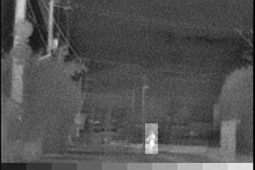
21 (a1) (a2) (a3) (a) Sequence 1: brightness-based segmentation + Histogram-based classification (b1) (b2) (b3) (b) Sequence 2: brightness-based segmentation + Histogram/Inertial-based classification (c1) (c2) (c3) (c) Sequence 3: bodyline-based segmentation + Histogram/inertial/contrast-based classification Fig. 17. Pedestrian detection performance for Sequence 1, 2, and 3. (a1)(b1)(c1): original images. (a2)(b2)(c2): Segmentation results. (a3)(b3)(c3): Classification results. 21