Fast Star Tracker Centroid Algorithm for High Performance CubeSat with Air Bearing Validation. Matthew Knutson, David Miller. June 2012 SSL # 5-12

Transcription

1 Fast Star Tracker Centroid Algorithm for High Performance CubeSat with Air Bearing Validation Matthew Knutson, David Miller June 2012 SSL # 5-12

2

3 Fast Star Tracker Centroid Algorithm for High Performance CubeSat with Air Bearing Validation Matthew Knutson, David Miller June 2012 SSL # 5-12 This work is based on the unaltered text of the thesis by Matthew Knutson submitted to the Department of Aeronautics and Astronautics in partial fulfillment of the requirements for the degree of Master of Science in Aeronautics and Astronautics at the Massachusetts Institute of Technology. 1

4 2

5 Fast Star Tracker Centroid Algorithm for High Performance CubeSat with Air Bearing Validation ABSTRACT by Matthew W. Knutson Submitted to the Department of Aeronautics and Astronautics on May 24, 2012 in Partial Fulfillment of the Requirements for the Degree of Master of Science in Aeronautics and Astronautics State of the art CubeSats such as ExoplanetSat require pointing precision for the science payload on the order of arcseconds. ExoplanetSat uses dual stage control to achieve the pointing requirement. Reaction wheels provide coarse satellite attitude control while a high bandwidth piezoelectric stage performs fine optical stabilization. The optical sensor provides star images from which a centroiding algorithm estimates the star locations on the optical focal plane. The star locations are used for both the optical control loop and satellite attitude determination. The centroiding algorithm requires a short processing time to maximize the bandwidth of the fine control loop. This thesis proposes a new fast centroiding algorithm based on centroid window tracking. The tracking algorithm utilizes centroid data from previous image frames to estimate the motion of the optical sensor. The estimated motion provides a prediction of the current centroid locations. An image window is centered at each predicted star location. A center of mass calculation is performed on the image window to determine the centroid location. This proposed algorithm is shown to reduce the computation time by a factor of 10 with a novel air bearing hardware testbed. This thesis also develops a high fidelity optical imager model in MATLAB Simulink. This model can be used to test centroiding algorithms and to simulate optical systems in a spacecraft pointing simulator. The model is validated with the air bearing testbed. Furthermore, the model is autocoded to C-code which is compatible with a rapid Monte Carlo analysis framework. Thesis Supervisor: Sungyung Lim Title: Senior Member of the Technical Staff, Charles Stark Draper Laboratory Thesis Supervisor: David W. Miller Title: Professor of Aeronautics and Astronautics DISCLAIMER: The views expressed in this thesis are those of the author and do not reflect the official policy or position of the United States Air Force, Department of Defense, or the U.S. Government. 3

6 Acknowledgements This work was performed primarily under contract with Draper Laboratory as part of the Draper Laboratory Fellowship Program. This work was also performed for contract FA with the Air Force Space and Missile Systems Center as part of the Space Engineering Academy. The author gratefully thanks the sponsors for their generous support that enabled this research. 4

7 Table of Contents 1. Introduction Background Problem Statement Literature Review Thesis Objectives and Approach Thesis Outline Algorithm Development Centroiding Algorithm Development Centroiding Algorithm Motivation and Purpose Centroiding Algorithm Traditional Approach Centroiding Algorithm Implementation Centroiding Algorithm Visualization Centroiding Algorithm Parameters Centroiding Algorithm Detailed Steps Traditional and Current Approach Comparison Tracking Algorithm Development Tracking Algorithm Motivation and Purpose Computationally Intensive Approach Overview Simplified Tracking Algorithm Derivation Tracking Algorithm Steps Tracking Algorithm Analysis Tracking Simulation Overview Analysis: Number of Centroids Analysis: Star Tracker Slew Star Tracker Simulation Motivation and Purpose Star Tracker Noise Sources

8 Noise Sources Overview Optics Model Overview Detector Noise Overview Star Tracker Model Implementation Implementation Overview Detector Model Detector Model Overview Point Spread Function Star Light Photon Count Clean Full Frame Image Stray Light Photon Count Electron Noise ADU Noise Star Tracker Model Output Fast Centroiding Algorithm Fast Centroiding Algorithm Software Architecture Fast Centroiding Algorithm Challenges Fast Centroiding Algorithm Overview Fast Centroiding Algorithm Step-by-Step Details Star ID Algorithm Star ID Algorithm Motivation and Purpose Star ID Algorithm Details Combined Star Tracker Model and Algorithms Centroid Accuracy Analysis Air Bearing Testbed Purpose and Objectives Testbed Set-Up Hardware Architecture Software Architecture Testbed Data Collection Procedures Testbed Data Analysis Analysis: Centroid Processing Time

9 Analysis: Air Bearing Motion Analysis: Centroid Prediction Error Star Tracker Model Validation Validation Future Work Monte Carlo Analysis Motivation and Background Matlab AutoCoder Draper Autocode Tools Tunable Parameters Monte Carlo Set-Up Autocode Validation Monte Carlo Analysis and Validation Conclusion Summary Future Work References

10 List of Figures Figure 1-1: ExoplanetSat Prototype [3] Figure 1-2: ExoplanetSat Payload Optical System [3] Figure 1-3: ExoplanetSat Focal Plane Array Layout [3] Figure 2-1: Example Camera Image with Centroid Code Figure 2-2: Pin Hole Camera Model [13] Figure 2-3: Block Diagram of Simulink Tracking Algorithm Analysis Figure 2-4: Tracking Code Angular Velocity Estimation Error vs. Number of Stars without Centroid Noise Figure 2-5: Tracking Code Angular Velocity Estimation Error vs. Number of Stars with 0.1 Pixel Standard Deviation Centroid Noise Figure 2-6: Tracking Code Angular Velocity Estimation Error vs. Angular Rate without Centroid Noise36 Figure 2-7: Tracking Code Angular Velocity Estimation Error vs. Angular Rate with 0.1 Pixel Standard Deviation Centroid Noise Figure 2-8: Tracking Code Centroid Prediction Error vs. Angular Rate without Centroid Noise Figure 2-9: Tracking Code Centroid Prediction Error vs. Angular Rate with 0.1 Pixel Standard Deviation Centroid Noise Figure 3-1: Star Tracker Model Error Tree Figure 3-2: High Level Block Diagram of Star Tracker Simulation Figure 3-3: Detailed Block Diagram of Optics Model Figure 3-4: Detailed Block Diagram of Detector Model Figure 4-1: High Level Software Architecture for Fast Centroiding Algorithm Figure 4-2: Detailed Software Architecture for Fast Centroiding Algorithm Figure 4-3: Example of Star ID Algorithm Figure 4-4: Combined Star Tracker Model and Fast Centroiding Algorithm Figure 4-5: Centroid Error vs. Spacecraft Rate with Stellar Aberration Off Figure 5-1 (a-f): Air Bearing Testbed Set-Up Figure 5-2: Avionics Hardware Architecture Figure 5-3: Air Bearing High Level Software Architecture Figure 5-4: Position of First Centroid over Time for ROI 200 Case Figure 5-5: Centroid 1 X Prediction Error vs. Estimated Angular Velocity Figure 5-6: Centroid 1 X Prediction Error vs. Estimated Angular Acceleration Figure 5-7: Centroid Prediction Error vs. Pitch Angular Velocity when Pitch Angular Acceleration is Below a Threshold Figure 5-8: Angular Velocity Bins Figure 5-9: Data Statistics for each Angular Velocity Bin with a Linear Best Fit Line through the Mean Standard Deviation Figure 5-10: Mean plus Standard Deviation Prediction Error vs. Slew Rate with Best Fit Line Figure 6-1: Monte Carlo Autocode Set-Up in MATLAB Figure 6-2: Autocode Monte Carlo Results

11 Figure 6-3: Simulink vs. Autocode Monte Carlo Results

12 List of Tables Table 3-1: Cypress HAS 2 CMOS Data Sheet Values [23] Table 4-1: Centroid Error with Stellar Aberration Off Table 4-2: Centroid Error with Stellar Aberration On Table 5-1: Centroid Processing Time Table 6-1: Autocode Validation

13 List of Acronyms ADCS ADU CCD CMOS COM FWHM ID ktc LIS MBD MEMS PIL PRNU PSF ROI SWIL Attitude Determination and Control System Analog-to-Digital Unit Charge-Coupled Device Complementary Metal-Oxide-Semiconductor Center of Mass Full Width at Half Maximum Identification Thermal Lost-in-Space Model-Based Design Micro-Electro-Mechanical Systems Processor-in-the-Loop Photo Response Non-Uniformity Point Spread Function Region of Interest Software-in-the-Loop 11

14 Chapter 1 1. Introduction 1.1. Background The CubeSat was originally conceived as a low cost alternative to provide universities with the ability to access space. When CubeSats were first conceived, their primary purpose was to provide hands on education to undergraduate and graduate students on the development of space hardware. Recently, they have evolved to play a more dominant role in scientific research. The scientific objectives often levy the requirement for high precision pointing of the science payload. There are several examples which highlight the need for high precision pointing space systems [1, 5, 8]. One example is ExoplanetSat which is a 3U (10cm x 10cm x 30cm) CubeSat under development at Draper Laboratory and the Massachusetts Institute of Technology with a mission to search for Earth like exoplanets using the transit method [1]. This mission requires arcsecond level pointing for the optical payload. ExoplanetSat uses a dual stage control algorithm in which reaction wheels provide coarse attitude control at 4 Hz and a piezoelectric stage provides fine optical control at 12 Hz. The piezoelectric stage translates the focal plane with the charge-coupled device (CCD) and complementary metal-oxide-semiconductor (CMOS) detectors so that the images on the detectors are stabilized on the order of arcseconds. The translation command is created from the star centroid locations on the optical detectors. Figure 1-1 below shows the satellite prototype, Figure 1-2 shows the payload optical system, and Figure 1-3 shows the focal plane array layout. 12

15 Figure 1-1: ExoplanetSat Prototype [3] Figure 1-2: ExoplanetSat Payload Optical System [3] 13

16 Figure 1-3: ExoplanetSat Focal Plane Array Layout [3] The centroid locations must be calculated from the detector output at high rate to close the piezo stage control loop and to provide better spacecraft attitude and angular rate estimates using star tracker algorithms [3]. The high precision pointing system can also be used in other satellite applications such as high bandwidth communication [5, 6, 7] and formation flying [8]. High bandwidth communication uses very narrow beam widths requiring fine pointing systems on the order of up to a few arcseconds [5, 6, 7]. An example of formation flying is robotic assembly. Small autonomous satellites cooperatively assemble a large space system such as a modular optical telescope [8]. This assembly requires a precise pointing system to fit each component into place Problem Statement The centroid algorithm takes significant computation time to produce centroid output from the detected star image. The computation time delay affects the pointing accuracy of the 14

17 dual stage control. In particular, this time delay limits the bandwidth of the fine optical control loop, thereby reducing pointing precision. Therefore, it is imperative to minimize the processing time of the centroid algorithm in the dual stage control. Another benefit of a fast centroiding algorithm is more accurate attitude determination with optical star measurements. These measurements are processed by star tracker algorithms to provide attitude estimates. For high precision pointing satellites, attitude estimates are often augmented by gyroscope rate measurements. However, micro-electro-mechanical systems (MEMS) gyroscopes for CubeSats are currently too noisy. A star tracker with a fast centroiding algorithm can provide accurate attitude rate estimates, therefore eliminating the need for a gyroscope. The processing time of the centroiding algorithm is affected by the processor speed and the algorithm efficiency. A dedicated high performance flight processor can reduce the centroiding algorithm processing time. However, CubeSats may not be able to support the additional cost, size, mass, volume, and power of a dedicated processor. Therefore, the preferred solution for CubeSats is to improve the centroiding algorithm efficiency Literature Review Ref [9] provides an excellent overview of how star trackers operate. The star tracker consists of three components: image data pre-processing, centroiding, and attitude determination. The centroiding algorithm processes the image data and produces the center locations of each star in the image. The reference proposes a two-phase operation including lost-in-space (LIS) and tracking to reduce computation time. The LIS mode processes the full frame image data to determine the centroid locations. The tracking mode uses the previous centroid data to predict 15

18 the location of the stars in the current image. Small centroid windows are defined at the predicted star locations. A center of mass algorithm is applied over these windows to measure the centroid locations. This method may speed up the centroiding algorithm and thus star tracker processing. However, the reference does not provide a tracking algorithm. Ref [15] presents a tracking algorithm based on an iterative least square estimation of star tracker attitude with optical measurements. The attitude is then used to define centroid windows. The reference assumes that the rotation between frames is small and the star tracker is modeled as a pin-hole camera. However, there is no end-to-end hardware implementation. Refs [13, 14] propose estimation of attitude and attitude rate with optical star measurements via an extended Kalman filter. This approach improves the attitude rate estimate. However, it is not applicable to the dual stage control which requires fast algorithms to achieve high precision optical pointing. There are many references which focus on accuracy of the centroid algorithms and modeling of the optical detectors. Refs [10, 11, 12] characterize the systematic errors of centroid algorithms and analyze the effect of the centroid point spread function (PSF). Refs [17, 18, 19, 20] describe modeling of the CCD and CMOS detectors Thesis Objectives and Approach The primary objective of this thesis is to develop a fast centroiding algorithm and demonstrate the performance on end-to-end hardware. The fast centroiding algorithm uses the two-stage approach [9] with the tracking algorithm developed by [15]. The tracking algorithm uses centroid data from previous images to estimate the slew rate of the optical system. The rate 16

19 estimate propagates the centroid locations forward to predict their locations in the current image. Small image windows are centered at the predicted locations. A center of mass (COM) centroid algorithm is calculated over the windows to determine the estimated centroid locations. Computation time is reduced because the centroid algorithm is not executed over the entire image. The tracking algorithm is further optimized to reduce the computation time. First, the suggested iteration is removed because the satellite attitude rate is small relative to the high image frame rate of the optical system. Second, the least square solution is found by a computationally efficient analytic formula of the pseudo-inverse. The tracking algorithm is also enhanced with a simple and robust star identification algorithm to track the same star between image frames. This algorithm is not based on the standard star tracking algorithm which matches stars from the image to a star catalog but a feature matching algorithm which directly compares stars from successive image frames. More importantly, the fast centroiding algorithm developed in this thesis is integrated with a hardware testbed assembled with camera, imager, artificial star field, and embedded processor. The algorithm is tested to analyze the real time performance in a dynamic slew environment similar to what the satellite will experience in space. This enables inexpensive validation of flight performance necessary to ensure mission success. The second objective of this thesis is to develop a high-fidelity star tracker image model in MATLAB Simulink. High-fidelity simulations offer a low cost platform for conducting hardware trade studies and predicting system performance before building engineering models and testbeds. The star tracker model simulates various noise sources which affect the optical 17

20 system [19, 20]. This model is validated with the hardware testbed data. The star tracker model is then integrated with the developed centroiding algorithm to analyze the performance in a software-in-the-loop (SWIL) testbed. Future work can use the SWIL testbed to validate further algorithm development before hardware implementation. The star tracker model is written in MATLAB Simulink for inexpensive development and maintenance. However, it is computationally expensive to simulate. Therefore, it is autocoded to C-code using a model-based design (MBD) framework developed at Draper Laboratory. This framework enables rapid development and test because algorithm updates are made in Simulink then quickly implemented and tested in C Thesis Outline This thesis is organized as follows. Chapter 2 provides the fundamentals of centroiding algorithms and develops the new fast centroiding algorithm. Chapter 3 develops the high-fidelity star tracker model which simulates the optical system. The model outputs simulated star field images which incorporate several optical and detector noise sources in order to mimic the actual hardware. Chapter 4 presents the software architecture for the fast centroiding algorithm. The software architecture integrates the fast centroiding algorithm, star tracker model, and star identification algorithm. This chapter also presents results of the centroiding algorithm performance analysis. Chapter 5 describes the air bearing testbed and performance of the fast centroiding algorithm. This chapter also presents validation of the star tracker model using the testbed results. Finally, Chapter 6 presents the MBD framework which enables rapid Monte Carlo analysis in a SWIL testbed. 18

21 Chapter 2 2. Algorithm Development 2.1. Centroiding Algorithm Development Centroiding Algorithm Motivation and Purpose A centroiding algorithm measures the star locations in the optical detector. The fine optical control loop uses the star locations to determine the piezo stage commands to stabilize the science star image. The centroids are also used for satellite attitude determination. Attitude determination is based on matching stars from the camera image to the star catalogue. Several sources of noise are introduced in the process of converting an image to an attitude measurement including detector noise, time delay, and star catalogue errors [9]. Errors in the centroiding algorithm along with detector noise will produce errors in the measured centroid location. Centroid errors can also cause improper matches to the star catalogue leading to attitude determination error. Therefore, it is important to utilize an accurate centroiding algorithm robust to detector noise. The processing speed of the centroiding algorithm is also an important consideration. Time delays limit the optical pointing precision. Some image processing techniques may improve the accuracy of the centroiding algorithm at the expense of increased processing time. Therefore, it may be necessary to trade centroid error and centroiding algorithm processing speed. 19

22 Centroiding Algorithm Traditional Approach The most common approach to determining the star locations is a simple COM algorithm [9]. The reference recommends a centroiding algorithm which checks every pixel in the image and compares it to a threshold value. If a pixel is above the threshold, a square region of interest (ROI) is identified with the detected pixel at the center. The value of the ROI border pixels are averaged and subtracted from each pixel within the ROI. This process subtracts out the background noise. A COM calculation is then used to find the centroid location within the ROI Centroiding Algorithm Implementation Centroiding Algorithm Visualization The centroiding algorithm utilized in this thesis is similar to Ref [9]. Figure 2-1 below shows an example of the centroiding algorithm used to find the center of a star on a camera image. 20

23 Figure 2-1: Example Camera Image with Centroid Code The white square boxes in Figure 2-1 represent the pixel number while the number in the center of each box represents the pixel value. The dotted red line represents the ROI. Two coordinate systems are shown: the pixel row-column value and the x-y Cartesian value. It is important to note that the centroid code is written in the C programming language. The pixel-column values begin with zero because array indexing in C begins with zero Centroiding Algorithm Parameters The centroiding code has three pre-defined variables including the signal threshold, noise threshold, and ROI size. The signal threshold is set to a bright pixel value indicating the presence of a star. The noise threshold is set to a value just above the noise floor. Simulation, lab, and calibration tests during flight can be used to determine threshold and ROI values. The ROI must be an even number. In the example shown in Figure 2-1 the signal threshold is 95, the noise threshold is 34, and the ROI is 6 pixels. The image size is 15 columns by 11 rows. The 21

24 image pixel values are stored in an array in C which can be visualized as a matrix. Each element in the matrix is equal to the corresponding pixel value Centroiding Algorithm Detailed Steps The centroiding code first checks each pixel to see if it is above the signal threshold. If the checked pixel is above the signal threshold, the ROI is centered on the pixel. The following center of mass (COM) calculation is used to find the centroid of the star. Only pixels that are above the nose threshold are included in the COM calculation. Notice that the noise threshold is subtracted from each pixel value. (2-1) (2-2) (2-3) where the centroid location is defined as with origin at the top left corner of the image; DN is the ROI brightness;,,, and refer to the starting pixel row value, ending pixel row value, starting pixel column value, and ending pixel column value of the region of interest; refers to the pixel intensity value at location (j,i) where j is the column value and i is the row value; is the noise threshold. Eqs 2-2 and 2-3 add 0.5 pixels to the x and y centroid positions in order to transform the coordinate system from the pixel row and column values to the Cartesian x and y values. Because C-language treats matrices as arrays the image is stored in an array with the number of 22

25 elements equal to the image width times the image height. In this example the image is stored in an array called I with 15 x 11 = 165 elements. The first pixel is at index 0 and the last pixel is at index 164 as shown in Figure 2-1. Therefore, the value of each pixel is accessed with an array element index as in [ ]. The index is calculated from: (2-4) where W is the image width defined as the number of pixel columns For example, the brightest pixel in Figure 2-1 has a value of 103 and is located at column 8 row 6. The index value is (6 x 15) + 8 = 98. In C, this pixel would be referenced as I[98]. After the centroid code finds the centroid location within the ROI, the algorithm continues to check the remainder of the image for more centroids. Each time a pixel above the signal threshold is identified, the COM is calculated over the respective ROI. A separate array called ischecked equal to the size of the image keeps track of which pixels have already been checked. This array is initialized to all zeros. Once a pixel has been checked to see if it is above the signal threshold or included in the COM calculation, the corresponding array value is changed from 0 to 1. Therefore, as the centroiding algorithm searches for stars, a pixel must be above the signal threshold and must have a value of 0 in the ischecked array before the COM algorithm is calculated at its respective ROI Traditional and Current Approach Comparison There are two key differences between the centroiding algorithm presented in this thesis and Ref [9]. First, the algorithm in the reference determines the noise threshold by calculating the average value of the pixels lining the border of the ROI. In order to save computation time 23

26 by not having to calculate a new threshold value for each detected star, the centroiding algorithm presented in this thesis uses one pre-determined noise threshold value. The average value of the noise floor should remain consistent between images. Therefore, image calibration can set the noise threshold ahead of time. The second difference between the centroiding algorithms is that the reference subtracts the noise threshold from each pixel in the ROI then calculates the COM over the entire ROI. The COM algorithm in this thesis only includes pixels that are within the ROI and above the noise threshold. If a pixel is below the noise threshold, it is ignored. As shown in Eqs 2-2 and 2-3, the centroiding algorithm in this thesis saves computation time by subtracting the noise threshold and performing the COM calculation in one step Tracking Algorithm Development Tracking Algorithm Motivation and Purpose The centroiding algorithm processing time is crucial for achieving high precision optical pointing. Checking each pixel in the image to compare to the signal threshold takes significant computation time when dealing with detector sizes on the order of a megapixel or more. The method proposed in this thesis to speed up the centroiding algorithm is to use a centroid tracking algorithm. The centroid tracking algorithm uses the centroids from previous frames to estimate the star tracker slew. The slew estimate is used to predict the centroid locations in the current frame. The COM algorithm is calculated over a small window or ROI centered at the predicted locations in order to determine the measured centroid location. Computation time is reduced because the centroiding algorithm is not calculated over the entire image frame. The centroid tracking algorithm provides two capabilities. First, the algorithm predicts the location of the centroids in the current image by propagating the previous centroid positions with 24

27 the estimated rate. Predicting the centroid locations for each frame provides the capability to run the COM algorithm on small centroid windows therefore speeding up the centroiding algorithm. The prediction is fundamentally based on the optical detector estimated roll, pitch, and yaw angular rates. Second, the estimated angular rates are used in the fine optical control loop to stabilize the science star image. These rates can also be used in the spacecraft attitude Kalman filter, thereby eliminating the need for a gyro which is necessary for high precision pointing Computationally Intensive Approach Overview Ref [13] proposes two methods for estimating angular rate using a star tracker. The first method called the attitude dependent angular velocity estimation algorithm feeds the star tracker s attitude estimate into a Kalman filter which estimates the spacecraft angular rate. The second method called the attitude independent approach estimates the spacecraft angular rate based on the movement of the star centroids. At each frame, the star centroids can be used to calculate a star unit vector. See Figure 2-2 below. Assuming the star camera has a sufficiently high update rate compared to the spacecraft slew rate, the time derivative of the change in the star unit vector from frame to frame along with a least squares algorithm can be used to estimate attitude rate. First order and second order attitude independent approaches are considered. The reference concludes that the attitude independent approach is more accurate because it is not affected by attitude determination errors. The attitude dependent approach will require the attitude determination and control system (ADCS) algorithm to match stars from each frame to the star catalogue to determine the spacecraft attitude and then use a Kalman filter or back differencing to determine rate. This approach is too slow. The attitude independent approach is also too complex given its use of 25

28 least squares filters. In order to reduce the computation time, this thesis will utilize a modified version of the centroid tracking algorithm developed in Ref [15] which is essentially a simplified version of the attitude independent approach of Ref [13] Simplified Tracking Algorithm Derivation Ref [15] proposes a method for attitude estimation which can be used to estimate spacecraft rates. The equation for dq on page 5 of Ref [15] contains a sign error. Therefore, the equations for the centroid tracking algorithm are derived again. The equations reference Figure 2-2 below. Pin Hole Star Vector: [u,v,f] f v u z y x Detector Figure 2-2: Pin Hole Camera Model [13] 26

29 Each star centroid is measured in meters by its (u,v) coordinate in the detector fixed frame. Assuming a perfect camera pin-hole model, the unit vector for each star is calculated with Eq 2-5: [ ] [ ] (2-5) where f is the lens focal length Recall Euler s rotation from one reference frame to another: [ ] (2-6) [ ] [ ] (2-7) where is roll in radians about the x-axis, is pitch in radians about the y-axis, and is yaw in radians about the z-axis. Assuming the small angle approximation ; ; ;, Euler s equation can be reduced: [ ] [ ] (2-8) Therefore, the simplified formula for rotating unit vectors from one coordinate frame to another is: [ ] [ ] [ ] (2-9) Multiplication reveals formulas for the x, y and z component of each star: 27

30 (2-10) (2-11) (2-12) Eqs 2-10 through 2-12 are used to find equations for u and v: (2-13) (2-14) Eqs 2-13 and 2-14 are linearized by taking partial derivatives: First recall the quotient rule: ( ) ( ) ( ) (2-15) Next assume that for slow slew rates and a high camera frame rate:,, and. Take partial derivatives: ( ) ( ) (2-16) (2-17) 28

31 (2-18) (2-19) (2-20) (2-21) The partial derivatives are formed into the Jacobian matrix: [ ] (2-22) [ ] Using the Jacobian, it is possible to find the change in the u and v positions of the i th stars given the rotation angles: [ ] = [ ] [ ] (2-23) where is u of the i th star in the previous image; is v of the i th star in the previous image; ;. The goal of Eq 2-23 is to solve for roll, pitch, and yaw given and for each star. The system has three unknowns ( and knowns where n is the number of stars. Therefore, assuming at least two stars in each image, recall from linear algebra that the system is 29

32 over-determined. The best estimate of the solution for an over-determined system is found with the following equations [16]: (2-24) (2-25) where: u is an [n x 1] matrix of unknowns, b is an [m x 1] matrix of knowns, A is an [m x n] matrix with more equations than unknowns (m > n), and is an [n x 1] matrix of estimated unknowns. Therefore, the following equation solves for estimated roll, pitch, and yaw: [ ] ( [ ] [ ] ) [ ] [ ] (2-26) Eq 2-26 is solved in MATLAB using the analytic formula for the inverse matrix. Define [ ]. A will always have three columns and the number of rows equal to twice the number of stars because each star adds two rows to A. Define another matrix. M will always be a 3 x 3 matrix because A is n x 3. Define each element in matrix M: [ ]. The analytic inverse of matrix M is found as follows: (2-27) 30

33 (2-28) [ ] Therefore, Eq 2-26 is solved analytically as follows: [ ] [ ] [ ] [ ] [ ] Tracking Algorithm Steps The centroid tracking algorithm is summarized as follows: 1. Find the change in each stars position from the previous image (k-1) to the current image (k): ;. 2. Build the Jacobian matrix (see Eqs 2-22 and 2-23) where u and v are the positions of the stars in the previous image (k-1). 3. Solve Eq 2-26 for the estimated roll, pitch, and yaw of the optical detector where u and v are the positions of the stars in the previous image (k-1). This solves for the estimated rotation angles from the previous image position to the current image position. Dividing the rotation angles by the detector frame rate determines the estimated angular velocity about the optical detector. 4. Build the Jacobian matrix again this time using the u and v values for the stars in the current image (k). 31

34 5. Solve equation 2-23 using the newly build Jacobian and the estimated roll, pitch, and yaw rotation angles to find and of each star. These values are the estimated change in each star s position from the current image (k) to the next image (k+1). 6. Add and to the current star locations to find the estimated star locations in the next image. The estimated star locations can be used to focus the centroiding code on portions of the detector where the stars are expected to land instead of centroiding the entire image wasting computation time. and can also be used for the fine optical control loop Tracking Algorithm Analysis Tracking Simulation Overview A numerical analysis of the centroid tracking algorithm was conducted in MATLAB Simulink to determine its accuracy at estimating the roll, pitch, and yaw attitude angles of the optical detector from the previous image frame to the current image frame and predicting the centroid locations in the next image frame. Figure 2-3 shows a block diagram of the simulation set-up. Roll Rate Pitch Rate Yaw Rate Euler s Equation: Propagate Actual Star Locations Actual Star Locations Apply Centroid Noise Centroids With Noise Tracking Algorithm Estimated Roll Estimated Pitch Estimated Yaw Predicted Centroids Estimate Actual Star Locations Figure 2-3: Block Diagram of Simulink Tracking Algorithm Analysis The simulation is given a constant roll, pitch, and yaw attitude rate as well as initial centroid locations. Running at 12 Hz (the star tracker frame rate), the centroids are converted to unit vectors, propagated, and converted back to centroid coordinates using Eqs 2-5, 2-7, 2-13, and Gaussian random noise blocks with a mean of 0 pixels and a standard deviation of

35 pixels add random centroid noise to the actual star locations. The tracking code uses persistent variables to store the centroids from the previous image frame. As described in steps 1 through 6 of the tracking algorithm in section 2.2.4, the centroids from the current frame and previous frame are used to find an estimate of the roll, pitch, and yaw of the optical detector. This roll, pitch, and yaw estimate is used to predict the location of the centroids in the next image frame (predicted centroids estimate). The tracking algorithm is calculated using the actual centroids and the centroids with noise in order to analyze the effect of centroid errors Analysis: Number of Centroids The tracking algorithm is first analyzed to determine how the number of centroids on the detector affects the angular velocity estimation error. Simulations are run for 5 seconds with a spacecraft rotation rate of 30 degrees per minute. Each case varies the number of centroids which are randomly placed on the detector. Each case is run for 1,000 trials. The three sigma angular velocity estimation error (average plus three times the standard deviation of the 1,000 trials) is plotted for each case. Roll and pitch are defined as the off-boresight axes. Yaw is defined as the boresight axis. Figure 2-4 shows the results without centroid noise and Figure 2-5 shows the results with 0.1 pixel standard deviation centroid noise. 33

36 Figure 2-4: Tracking Code Angular Velocity Estimation Error vs. Number of Stars without Centroid Noise Figure 2-5: Tracking Code Angular Velocity Estimation Error vs. Number of Stars with 0.1 Pixel Standard Deviation Centroid Noise As the number of stars on the detector increases the angular velocity estimation error decreases non-linearly. When more than eight stars are present on the detector, adding additional stars has little effect on improving the angular velocity estimation error. The estimation error with 0.1 pixel centroid error is about 2.5 to 3 orders of magnitude greater than the error without centroid noise. Therefore, centroid noise contributes significantly to angular velocity estimation error. The results show that estimation error about the yaw axis is up to one order of magnitude greater than roll and pitch. This result is not surprising because the yaw axis is the boresight 34

37 axis, and star trackers are least accurate about boresight [9]. When centroid noise is considered, the error about boresight improves significantly with more than four stars. Further analysis will assume eight stars are on the detector Analysis: Star Tracker Slew Next, the tracking algorithm is analyzed to determine how the spacecraft rate affects the attitude rate estimation error and centroid prediction error. Each trial is run with 8 centroids randomly placed at initial locations on the detector. Each case varies the spacecraft rate. The simulation was not set-up to drop stars as they fall off the detector. Therefore, stars can move an infinite distance from the center of the detector and still be included in the tracking algorithm. So, as the spacecraft rate increases the simulation time was decreased to prevent stars moving too far from the center of the detector. Simulation time is an important consideration because the tracking algorithms were developed by linearizing the combined Euler and camera pin-hole equation (Eqs 2-13 and 2-14). As stars move further from the center of the detector, errors increase due to the non-linear nature of the equation. Because the stars were randomly placed on the detector, some stars were initially placed at the edge and therefore do move far enough from the center of the detector that they would normally fall off. However, these errors are minimized due to the 1,000 Monte Carlo trials. The three sigma attitude error is plotted for each case. Figure 2-6 and Figure 2-7 show the angular velocity estimation error. Figure 2-8 and Figure 2-9 show the errors in predicting the centroid locations. 35

38 Figure 2-6: Tracking Code Angular Velocity Estimation Error vs. Angular Rate without Centroid Noise Figure 2-7: Tracking Code Angular Velocity Estimation Error vs. Angular Rate with 0.1 Pixel Standard Deviation Centroid Noise Without centroid noise, attitude estimation error increases non-linearly. When centroid noise is factored into the tracking algorithm, the attitude estimation error is nearly constant as rate increases. Even with zero spacecraft rate, the attitude estimation error with centroid noise is several times greater than the attitude estimation error without centroid noise. Therefore, a centroid noise of just 0.1 pixels has a much larger effect on attitude estimation error than the spacecraft rate. The figures below show similar results for centroid prediction error. 36

39 Figure 2-8: Tracking Code Centroid Prediction Error vs. Angular Rate without Centroid Noise Figure 2-9: Tracking Code Centroid Prediction Error vs. Angular Rate with 0.1 Pixel Standard Deviation Centroid Noise An estimate of roll, pitch, and yaw rate is necessary to predict the new centroid locations as shown in Eq Therefore, the centroid prediction error is related to the attitude rate estimation error. Without centroid noise, as spacecraft rate increases, the prediction error increases non-linearly. With centroid noise, the prediction error is nearly constant. Again, 37

40 centroid noise is the dominant error source. With 0.1 pixel centroid error, the new centroid locations are predicted to within 0.4 pixels. 38

41 Chapter 3 3. Star Tracker Simulation 3.1. Motivation and Purpose When designing an optical high precision pointing system many factors contribute to the pointing performance. It may be necessary to consider several system architectures and trade several hardware options. One cost effective method to perform hardware trade studies and to analyze performance is to create a computer simulation of the optical hardware. There are several noise sources from the selected detector and theoretical optical limitations which affect the system performance. The simulation must be robust to capture the dominant noise sources which impact the downstream pointing precision. Therefore, the goal is to develop a robust model of the camera optics and detector in MATLAB Simulink. The model should generate simulated star field images which include optical and detector noise. The images can be analyzed with simulations to characterize the centroid error Star Tracker Noise Sources Noise Sources Overview There are several optical and detector noise sources that must be simulated in the camera model. For the purpose of organizing the simulation, the noise sources can be placed into categories as shown in the following error tree. The error tree is based on Refs [9, 18, 19, 20]. 39

42 Star Tracker Optics Detector Stellar Aberration Focal Plane Misalignments Photon Electron ADU Photon Point Spread Function Shot Noise Saturation Integration Time Fixed Pattern Noise Quantization Line Scan Aberration PRNU Lens Vignetting Loss and Throughput Dark Current Stray Light ktc Noise Read Noise Figure 3-1: Star Tracker Model Error Tree The noise sources are split into two main groups including optics and detector Optics Model Overview The optics model includes stellar aberration and focal plane misalignments. These error sources determine where a star lands on the detector. Stellar aberration is a distortion caused by the spacecraft absolute velocity (spacecraft orbital velocity plus Earth s orbital velocity) compared to the speed of light. Focal plane misalignments are errors between the actual location the detector is mounted and the modeled location. When building the spacecraft optical system, there will be small rotational and linear misalignment errors between the designed location and built location. These errors should have little effect on the pointing performance because the 40

43 software and star catalogue can be adjusted to model the actual location of the detector. The error that does matter is the error between where the detector is actually located and where we think it is located. This is a misalignment calibration error which does add noise to the model. The stellar aberration and misalignment calibration error add a bias to the centroid positions because these errors affect the actual location of the star on the detector before detector noise is applied Detector Noise Overview The detector model includes noise that affects the individual pixel values from the image. The detector group is split into three categories including photon, electron, and ADU. The pixels on a CMOS detector act like wells. When a photon strikes a pixel, an electron is produced. Throughout the duration of the integration time, the pixel wells fill up with electrons as more and more photons strike the pixel. When integration terminates, the CMOS electronics measure each pixel charge as a voltage. An analog-to-digital converter outputs the voltage reading as an analog-to-digital unit (ADU). The ADU count for each pixel is a measure of how much light fell on each pixel during the integration time [17, 18]. The image data is stored as a matrix with each element containing the ADU value of the corresponding pixel. Each group in the error tree detector category corresponds to one step in the detector imaging process. The photon group determines how many photons strike each pixel within the integration time. The electron group includes the error from electrical interference and noise as the photons are converted to electrons. The ADU group captures the error in converting from voltages to ADU counts. The photon group includes the photon point spread function (PSF), integration time, line scan aberration, lens vignetting loss and throughput, and stray light. Star light is defocused over 41

44 several pixels. The PSF is modeled as a Gaussian function which spreads the star light over several pixels. The integration time is similar to the shutter on a traditional camera. It determines how long the period of photon collection lasts for each image. A longer integration time results in more photons collected and a brighter image. Some detectors have a rolling shutter. This means that the camera is read out one row at a time. Therefore, there is a slight time delay from when the top and bottom rows are integrated. This effect is referred to as line scan aberration. Lens vignetting and throughput refer to loss of photons as they pass through the lens considering the lens is thicker at the edges compared to the center. Reflections from the moon, Earth, and other parts of the spacecraft will result in additional photons striking the detector. These photons are classified as stray light. The electron group includes shot noise, fixed pattern noise, photo response nonuniformity (PRNU), dark current, thermal (ktc) noise, and read noise. These error sources are all caused by electrical noise on the sensitive imager electronics. Some of the noise sources such as shot noise and dark current are Poisson distributions. However, a Gaussian distribution is a close approximation. Therefore, for simplicity, all the electrical noise sources are modeled as Gaussian. These noise sources depend on the specific detector and can be found in a data sheet or through hardware lab tests. The ADU group includes saturation and quantization. Each pixel can only accept a limited number of photons which results in a maximum ADU count. Long integration times can cause overexposure resulting in saturated pixels. Saturation increases centroid error because the shape of the star is degraded as the top of the Gaussian is essentially chopped off. Quantization occurs when the electrons are converted to ADU counts and rounded to the nearest ADU. 42

45 3.3. Star Tracker Model Implementation Implementation Overview The star tracker model is written in MATLAB Simulink for quick implementation and testing. In Chapter 6 it will be autocoded to C-code with a MBD framework developed at Draper Laboratory. The algorithm for simulating images is split into the two main categories from the error tree including the optics model and detector model. Figure 3-2 through Figure 3-4 show block diagrams of the star tracker simulation. S/C Slew Rate S/C Initial Attitude Quaternion Rate = 10*Integration Time Propagate Attitude Quaternion S/C Velocity S/C Attitude Quaternion Optics Model Buffer Star Locations on Image Buffer Off-Boresight Angles Rate = Integration Time Detector Model Simulated Image Star Unit Vectors Figure 3-2: High Level Block Diagram of Star Tracker Simulation S/C Attitude Quaternion S/C Velocity Star Unit Vectors Optics Model Apply stellar aberration Star Unit Vectors Calculate Off- Boresight Angles; Convert stars from unit vectors to star locations on imager Star Locations on Image Apply focal plane misalignments Off-Boresight Angles Star Locations on Image Buffer Data: Optics Rate = 10*Integration Time Imager Rate = Integration Time Buffer Star Locations on Image Buffer Off-Boresight Angles Figure 3-3: Detailed Block Diagram of Optics Model 43

46 Buffer Star Locations on Image Detector Model Buffer Off-Boresight Angles Generate a 5x5 pixel grid for each star, place star on grid considering line scan aberration, use Gaussian function to estimate point spread function 5x5 Pixel Grid Calculate number of photons on each pixel considering star magnitude, integration time, vignetting loss, and lens throughput 5x5 Pixel Grid Re-locate 5x5 grids to the full image frame Simulated Image Without Noise Apply stray light photons Simulated Image Convert to electrons and apply shot noise, dark current, PRNU noise, fixed pattern noise, read noise, and ktc noise Simulated Image Convert to ADU counts and apply saturation and quantization Simulated Image Figure 3-4: Detailed Block Diagram of Detector Model Start with Figure 3-2. The star tracker simulation first runs a MATLAB script which initializes a constant spacecraft slew rate and constant spacecraft absolute velocity. These values are initialized as vectors with three elements for the three spacecraft axes. The absolute velocity should change as the spacecraft orbits the earth. However, for the purpose of simplifying the simulation for parametric analysis, the velocity is specified as a constant. The MATLAB script also specifies the initial spacecraft attitude quaternion and the initial star locations. The star locations are unit vectors referenced to the detector. The first step of the Simulink model is to use the slew rate to update the spacecraft attitude quaternion. The second step is to run the optics model to determine the star centroid locations on the detector and off-boresight angles considering stellar aberration and detector misalignments. The off-boresight angles are used later to calculate vignetting. The last step is to run the detector model to produce a simulated image. 44

47 Notice the simulation runs at two different rates. Here rates are defined as simulation time steps in Hz. The detector model runs at the integration time while the propagate attitude quaternion and optics model run at 10 times the integration time. For example, assume the star tracker integration time is 83.3 milliseconds or 12 Hz. The detector model runs at 12 Hz and the optics model runs at 120 Hz. The purpose of the two rates is to account for stars smearing across the detector as the spacecraft slews during the integration time. The optics model runs 10 iterations (120 Hz / 12 Hz = 10) for every time the detector model generates a simulated image. The centroid locations and off-boresight angles produced from the optics model are stored in a buffer. The buffer holds up to 10 propagated star locations for each star on the detector. The buffer is then passed at 12 Hz to the detector model. Each time the detector model runs it has access to all the star locations as the stars slewed across the detector for the current image. In other words, for each image the stars slew across the detector for 83.3 milliseconds. By running the optics model at 120Hz we can discretize each smeared star into 10 discrete locations. The 10 discrete locations are passed to the detector model so that it can simulate the star smear Detector Model Detector Model Overview The detector model uses small pixel grids for each star in the buffer to simulate the PSF and photon count from the star. The grid is then placed in its corresponding location in the full frame image. Once all the grids for each centroid position are placed in the full frame image, the remaining detector noise is calculated on the full image. 45

48 Point Spread Function The first step in the detector model is to calculate the PSF of each propagated star location in the buffer. Refer to the first block in Figure 3-4. A small grid is used rather than the full image because the PSF of a star only covers a few pixels. The baseline grid size is 5x5 pixels. The PSF is simulated with a Gaussian function which is a close approximation to the actual star PSF. (3-1) (3-2) where is the Gaussian function solved at discrete points [ ] on the grid; [ ] where and are the coordinates for the center of the star; [ ] where is the standard deviation calculated as ; FWHM is the PSF full width at half maximum So, for each star location in the buffer, a Gaussian function is centered at the decimal location of the star at the middle of the 5x5 pixel grid. For example, if one centroid location in the buffer is (102.23, 54.78), the PSF is simulated in a 5x5 pixel grid at location (0.23, 0.78) in the center pixel. The goal is to solve the Gaussian function at each pixel in the grid. For improved accuracy, each pixel in the 5x5 grid is also divided into a sub-grid nominally 5x5. The Gaussian function is solved at the discrete sub-grid locations within each pixel. The value of each pixel equals the average value of the discrete locations within each pixel. Finally the pixel values are normalized by dividing each pixel by the sum of the pixels. In MATLAB code, the grid is saved as a 5x5 matrix. The value of each element corresponds to the pixel value. The 46

49 pixels are normalized because the Gaussian grid is used later as a weighting function to determine how many photons strike each pixel Star Light Photon Count The second step in the detector model is to calculate the number of photons that fall on each pixel in the 5x5 grid. Refer to the second block in Figure 3-4. Eqn 3-3 calculates the total number of photons that fall on each 5x5 grid. (3-3) (3-4) where is the total number of photons, is the flux vega, Mag is the star magnitude, A is the aperture area, is the throughput, is the vignetting loss, is the integration time, is the number of discrete centroid locations which equals 10 or (optics model rate / detector model rate), is the vignetting, and is the off-boresight angle Dividing by the number of buffered locations is necessary because a 5x5 grid is calculated for each propagated star location in the buffer. The numerator in Eq 3-3 calculates the total number of photons collected for each star on the full frame image. Dividing by the number of discrete locations that make up a star in the full frame image calculates the number of photons at each discrete propagated location. The next step is to create a 5x5 grid with each pixel value equal to the correct number of photons that make up a star. The photon grid is created by multiplying each pixel in the PSF grid by the total number of photons: (3-5) 47

50 where is the photon grid, G is the PSF grid calculated previously, is the total number of photons Therefore, the PSF grid is essentially used as a unique scale factor for each pixel in the grid to find the proportion of the total photons that land on each pixel Clean Full Frame Image Step three in Figure 3-4 is to relocate each photon grid to the proper star location in the full frame image. In the example above, one of the centroid locations in the buffered centroid list was at location (102.23, 54.78). The PSF was calculated with the Gaussian centered at location (0.23, 0.78) in the center pixel of the grid. The 5x5 photon grid needs to be placed such that the center pixel in the grid is located at (102, 54) in the full frame image. The full frame image is initialized as a matrix of zeros with row and column size corresponding to the full frame detector size. Each element in the matrix corresponds to a pixel value in the detector. Steps 1 through 3 in Figure 3-4 are repeated for each propagated centroid location in the buffered centroid list. Once complete, the full frame image is a matrix of zeros except at the centroid locations where the photon grids were injected. This matrix simulates what a star image would look like if there was no detector noise or stray light Stray Light Photon Count Step four of the detector model adds stray light to the clean image. The total number of stray light photons is calculated as follows: ( ) (3-6) 48

51 where is the total number of stray light photons, is the stray light multiplier, is the flux vega, zmag is the zodiacal light magnitude, A is the aperture area, is the throughput, is the integration time, cols is the total number of pixel columns and rows is the total number of pixel rows in the full frame image, is the focal length, and is a unit conversion for the number of radians in an arc second calculated as: The total number of stray light photons is added to every pixel in the clean image Electron Noise Step five is to convert the image to electrons then apply the detector noise shown in block 5 of Figure 3-4. The image is converted to electrons by multiplying each pixel by the efficiency value found in the data sheet. Once converted to electrons, various noise sources are modeled. (3-7) Shot noise: (3-8) Dark current: (3-9) PRNU: ( ) (3-10) Fixed pattern noise: 49

52 (3-11) Read noise: (3-12) ktc noise: (3-13) where is a matrix in which each element represents the corresponding pixel value in the full frame image, distinguishes the matrix before a specific noise is added, is the photon to electron conversion efficiency, is the dark current, is the integration time, is the PRNU noise, is the fixed pattern noise, is the read noise, is the ktc noise. The noise sources are modeled one at a time. For example, in order to simulate shot noise and dark current only, use Eq 3-8 to calculate shot noise then set I o equal to I and use Eq 3-9 to calculate dark current. Notice the noises are not calculated on separate images then added together. Instead, after shot noise was calculated, the shot noise image was used as I o in the calculation for dark current. The equations for detector noise introduced above are written in MATLAB syntax for ease of understanding. The multiplier refers to element by element multiplication and creates a matrix the same size as the image with each element equal to one. The detector noise is simulated as Gaussian random noise. The randn command in MATLAB generates a random number with mean and standard deviation equal to one. Multiplying randn by a constant creates a random number with standard deviation equal to the constant. Adding a constant to randn creates a random number with mean equal to the constant. 50

53 (3-14) The equation above creates a matrix the same size as the image called Gaussian Noise. Each element in the matrix was created from a random number generator with mean equal to Mean and standard deviation equal to σ. The standard deviation values used in Eqs 3-8 through 3-13 can be found in the detector data sheet provided by the manufacturer. Table 3-1 below shows values from the Cypress HAS 2 CMOS detector which are used as nominal values in the detector model. Table 3-1: Cypress HAS 2 CMOS Data Sheet Values [23] Cypress HAS 2 CMOS Data Sheet Values Characteristic Min Typ Max Unit Remarks Image sensor format N/A 1024 x 1024 N/A pixels Pixel Size N/A 18 N/A µm Spectral Response (Quantum efficiency x Fillfactor) N/A 33.3 N/A % Measured average over nm Global fixed pattern noise standard deviation (Hard N/A e- With DR/DS reset) Global photo response non uniformity, standard deviation N/A % Of average response Average dark signal N/A e-/s At 25 ± 2 C die temp, BOL Temporal noise (NDR Soft reset) N/A e- read noise ktc noise N/A 0 N/A e- zero when running in Correlated Double Sampling-Non-Destructive Readout mode Charge to voltage conversion factor µv/e- Output amplifier gain N/A 1 N/A ADC ideal input range 0.85 N/A 2.0 V voltage swing: ADC resolution N/A 12 N/A bit 10 bit accuracy at 5 Msamples / sec When the simulation is run, new random numbers are generated for each image with the exception of PRNU and fixed pattern noise. PRNU and fixed pattern noise are characterized as random noise however they remain constant for each image once the detector is turned on. Therefore, the random number matrices for PRNU and fixed pattern noises are generated once at 51

54 the start of the simulation using persistent variables. Eqs 3-10 and 3-11 show the MATLAB syntax Randn with a capital R to indicate this difference ADU Noise Step 6 is to convert the image from electrons to ADU counts and apply saturation and quantization. The image is converted to ADU counts as follows: (3-15) where is the resolution, is the voltage swing, is the amplifier gain, and is the charge to voltage conversion Saturation is accounted for by setting the minimum pixel value to zero and the maximum pixel value to. Quantization is simulated by rounding each pixel value to the nearest integer Star Tracker Model Output The output of the star tracker model is a simulated star field image. This image is passed to the software which runs a centroiding algorithm to determine the centroid locations. The noise values that contributed to building the image will affect the centroid error. In order to accurately characterize the centroid error, the images need to be validated for accuracy. Validation can occur through the use of hardware testbeds by taking actual images and comparing to the simulated images. 52

55 Chapter 4 4. Fast Centroiding Algorithm 4.1. Fast Centroiding Algorithm Software Architecture Fast Centroiding Algorithm Challenges In order to develop a fast centroiding algorithm based on the tracking algorithm described in Section 2.2, several factors had to be considered. First, the tracking algorithm uses the centroid locations from the previous images to predict the centroid locations in the current image. The tracking code must be initialized with centroids. Second, the tracking code requires at least four stars for adequate attitude rate accuracy. The tracking code must handle cases in which too few stars land on the detector as stars are added and subtracted due to the star tracker slew. Third, the tracking code must subtract the current centroid locations from the previous locations. The centroid code reads out centroids in order from the top of the image to the bottom of the image. With this constraint, the tracking code must match stars from the current frame to the previous frame when the order of the centroids changes and stars are added or subtracted due to the star tracker slew Fast Centroiding Algorithm Overview Figure 4-1 below shows a high level block diagram of the fast centroiding algorithm software architecture. Figure 4-2 below shows the software architecture in more detail. 53

56 First Image State 1 No If Num Cntrds > 3 Yes State 10 No If Num Cntrds > 3 and Error Flag = 0 State 2 Yes No If Num Cntrds > 3 Yes Figure 4-1: High Level Software Architecture for Fast Centroiding Algorithm 54

57 55

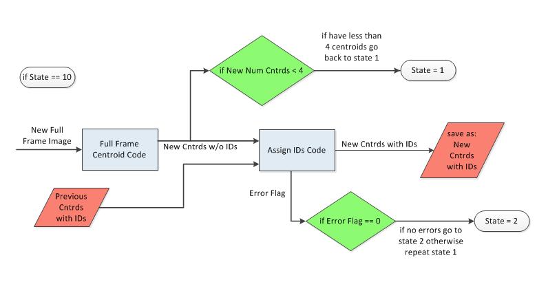
58 Figure 4-2: Detailed Software Architecture for Fast Centroiding Algorithm The fast centroiding algorithm has three states that are called by a switch case statement in C-code: state 1, state 10, and state 2. The state value is saved as a global variable. Each time the star tracker takes an image, the current state is executed. Organizing the code into multiple states adds the ability for the fast centroiding algorithm to respond to the dynamic environment of an Earth orbiting spacecraft. As stars are added and subtracted from the detector, the algorithm can determine which state should be executed in the next image frame. Two new functions are included in this architecture. First, the centroiding code is split into a full frame centroiding algorithm and a windowed centroiding algorithm. The full frame centroiding algorithm used for the LIS mode searches the entire image frame for centroids as described in section The tracking algorithm executed during the tracking mode uses centroid data from previous image frames to determine the predicted centroid locations in the current image frame. The windowed centroiding algorithm runs the COM calculation on image windows centered at the predicted star locations. Therefore, the windowed centroiding algorithm 56

59 differs from the full frame centroiding algorithms because it does not use a signal threshold to determine each ROI location. Because the windowed algorithm does not search the entire image for centroids, the processing time required to output centroids from each image is significantly reduced. Another function added to the software architecture is a star identification algorithm. This algorithm assigns an identification (ID) number to each star read out from the centroid code. As stars are retired, the IDs for those stars are retired and as stars are added they are assigned new IDs. The tracking code uses the star IDs to accurately match stars from the current frame to the previous frame when estimating star tracker slew rate Fast Centroiding Algorithm Step-by-Step Details The algorithm initializes to state 1 (LIS mode). State 1 runs the full frame centroiding algorithm. The new centroids are passed to a function called Assign First Time Star IDs. The centroid data is saved in a global variable called Previous Centroids. If the centroid code found four or more stars, the next image will move on to state 10 (transition mode from LIS to tracking mode). If there are less than four centroids, the next image will repeat state 1. State 10 runs the full frame centroid code then passes the new centroids and the previous centroids to the Assign IDs function. This function matches the stars in the current image to the stars in the previous image. Matching stars are given identical ID numbers, IDs for retired stars are dropped, and new IDs are assigned for new stars. The new centroid data and IDs are saved in a global variable called New Centroids. If there are four or more new centroids and no error flag from the ID code, the state is set to 2, otherwise the state is re-set to 1. State 2 (tracking mode) passes the centroids and IDs from the previous two images to the tracking code which predicts the 57

60 location of the stars in the current image. The windowed centroid code uses the predicted centroid locations to find the new centroids in the current image. If the windowed centroid code finds fewer than four stars, the state is reset to one. Otherwise, the state remains at 2 and the new centroids and previous centroids are saved Star ID Algorithm Star ID Algorithm Motivation and Purpose The purpose of assigning star IDs is to handle cases in which stars are added or subtracted from the image. The centroid code saves centroid data in an array with 20 elements as follows: [ ]. The first element in the array is the u centroid value of the first star, the second element is the v centroid value of the first star, the third position is the u centroid value of the second star, and the fourth position is the v centroid value of the second star. This pattern continues for up to 10 stars. The centroid code stops saving centroid data if more than 10 stars are found. Because the centroid code always reads from the top of the image to the bottom, as stars are added or subtracted during spacecraft slew the order of the centroids changes. Figure 4-3 below demonstrates this problem. 58

61 First Full Frame Image Second Full Frame Image (0,0) u-axis (0,0) u-axis U 1 (k),v 1 (k) v-axis U 1 (k-1),v 1 (k-1) v-axis U 3 (k),v 3 (k) U 2 (k-1),v 2 (k-1) U 2 (k),v 2 (k) Figure 4-3: Example of Star ID Algorithm As the star tracker slews between reading out the first and second image, the first and second star move positions and a third star is added. The centroid code will read out the centroid positions for each frame as follows: [ ] and [ ]. The tracking code needs to find the change in position for each star ( and ) from the first image frame to the second image frame. Because the order of the centroids changes, the tracking code cannot simply subtract the C(k) array from the C(k-1) array. This thesis develops a simple and robust star ID algorithm based on angular distance of images without a priori information such as a star catalog Star ID Algorithm Details State 1 uses the Assign First Time Star IDs algorithm to create star IDs for the first full frame image. This function simply assigns IDs in numerical order. The first centroid is given ID number 1, the second centroid is assigned ID number 2, and so on, for each star the centroid code finds up to a max of 10. In the example shown in Figure 4-3, for the first frame image, star ( ) is given ID 1 and star ( ) is given ID 2. 59

62 State 10 uses the Assign IDs algorithm to assign IDs to the centroids found in the second full frame image. This algorithm must correctly match each star in the current image frame to a star from the previous image. Assuming the spacecraft slews at a slow rate relative to the star tracker frame rate, the stars will only move a small distance between images. Therefore, the Assign IDs algorithm subtracts each star s current location from all the star locations in the previous frame. Whichever star pair has the smallest displacement is considered a match. For the example shown in Figure 4-3, the star ID for star in the second full frame image is found by calculating the following displacements: and. The smallest distance represents a match to star ( ). In this example, will be smaller than, therefore star ( ) matches star ( ). Star ( ) is assigned ID 1 to match the ID assigned to star ( ) in the Assign First Time Star IDs function explained above. There is no need to take the square root in the distance equation because the ID algorithm does not have to find the actual distance between stars in order to identify matches. Leaving out the square root saves computation time. In order to account for cases in which stars are added or retired between images, a threshold called maxdeltauv is used to specify the maximum distance allowed between star matches. If the distance between a star in the current frame and star in the previous frame is greater than the threshold, the pair is ruled out as a match. For example, the Assign IDs code will find the distances between star ( ) in the second image and both stars in the first image. If both distances are greater than the threshold, it is assumed that star ( ) was added due to the spacecraft slew and is assigned ID 3. 60

63 There are two cases in which the ID algorithm could fail triggering the output of an error flag. The first error occurs if fewer than two star matches are detected because the tracking code needs at least two star pairs in order to estimate slew rate. The second error occurs when one star from the previous frame is matched to more than one star in the new frame. This can happen if stars become clustered together. As shown in Figure 4-2, any errors will trigger the software architecture to return to state 1 and start over Combined Star Tracker Model and Algorithms The fast centroiding algorithm was combined with the star tracker model into a MATLAB Simulink simulation as shown in Figure 4-4 below. S/C Slew Rate S/C Initial Attitude Quaternion Propagate Attitude Quaternion S/C Attitude Quaternion Optics Model Centroids Off Boresight Angles Detector Model Simulated Image Fast Centroiding Software Measured Centroids Predicted Centroids Estimated S/C Rate Figure 4-4: Combined Star Tracker Model and Fast Centroiding Algorithm The simulation initializes a constant slew rate, spacecraft attitude quaternion, and star locations on the detector. The spacecraft attitude is propagated with the slew rate at each simulation time step. The optics model and detector model create a simulated camera image as explained in 61

64 Chapter 3. The simulated image is passed to the fast centroiding software to output the measured centroids, predicted centroids, and estimated star tracker slew rate Centroid Accuracy Analysis The centroiding algorithm accuracy was tested with Monte Carlo runs from the star tracker simulation. For each trial, one star was placed at a random location on the detector. The optics and detector model simulated a camera image which was passed to the fast centroiding code. The fast centroiding algorithm was modified so that only the full frame centroiding algorithm was used to calculate the measured centroid location. A parametric analysis was conducted varying the slew rate from 0 to 0.5 deg/sec. Each trial was run 100 times in order to provide enough data for statistical analysis of the centroid error. Centroid error is defined as the difference between the actual centroid location and the measured centroid location. Two different cases were tested: stellar aberration on and off. A constant spacecraft orbital velocity was used in the optics model to determine the stellar aberration. The results are shown in the tables below. Table 4-1: Centroid Error with Stellar Aberration Off Star Tracker Model Centroid Error Analysis (stellar aberration off) Slew Rate (deg/sec) X Centroid Error (pixels) Y Centroid Error (pixels) Roll Pitch Yaw Mean Std Dev Mean Std Dev E E E E E E E E E E E E E E E E E E E E n/a n/a n/a n/a 62

65 Table 4-2: Centroid Error with Stellar Aberration On Star Tracker Model Centroid Error Analysis (stellar aberration on) Slew Rate (deg/sec) X Centroid Error (pixels) Y Centroid Error (pixels) Roll Pitch Yaw Mean Std Dev Mean Std Dev E E E E E E E E E E E E E E E E E E E E n/a n/a n/a n/a Table 4-1 and Table 4-2 show the centroid error with and without the stellar aberration respectively. Figure 4-5 below shows the standard deviation of the centroid error with the stellar aberration turned off. Figure 4-5: Centroid Error vs. Spacecraft Rate with Stellar Aberration Off 63

66 The data shows that the centroid error standard deviation increases as rate increases. As the spacecraft slew rate increases, the star smears across the detector. This smear increases the centroid error because of two effects. First, the elongated shape reduces the star s symmetry. Second, as smear increases, the star becomes dimmer reducing the signal to noise ratio. If the brightest pixel drops below the centroiding algorithm signal threshold, the centroiding algorithm will fail to identify a star. This effect is shown in the results for 0.5 deg/sec which are n/a because the centroid code failed to detect the star. Stellar aberration does not affect the standard deviation as it is nearly the same for both cases. However, stellar aberration does affect the mean centroid error. The mean is nearly zero when the stellar aberration is off and on the order of 0.5 pixels when the stellar aberration is on. This result makes intuitive sense because stellar aberration shifts the star location on the detector in the optics model. This has the effect of introducing a bias in the centroid error. The stellar aberration centroid error is greater in the x direction due to the constant velocity chosen for the simulation. In flight, the spacecraft velocity would change depending on the satellite s orbital location resulting in a varying mean centroid error. The goal of these results was to use a constant velocity representative of flight to provide typical error values. 64

67 Chapter 5 5. Air Bearing Testbed 5.1. Purpose and Objectives A hardware testbed was developed in order to complete two objectives. The first objective was to measure the critical performance metrics of the fast centroiding algorithm such as processing time and centroid prediction error in a flight-like dynamic slew environment. The second objective was to use a relatively low cost testbed to validate the star tracker model. Once validated, the model can be used in a SWIL testbed in order to develop and analyze further attitude control algorithms before hardware validation. For example, the model can be combined with a high fidelity spacecraft simulation which provides a low cost platform for conducting trade studies, developing flight software via MALAB AutoCoder, and analyzing the optical pointing performance to determine if it can meet scientific objectives Testbed Set-Up Hardware Architecture Demonstrating the performance of the fast centroiding algorithm requires the ability to rotate the star tracker in order to displace stars to different locations on the detector. It was determined that a three degree of freedom air bearing could fulfill this requirement. An air bearing is a device often used to test spacecraft attitude determination and control systems. A platform is mounted on a support column. Air is pumped through the column to levitate the 65

68 platform allowing for 360 degree rotation about the axis running through the support column and approximately 45 degree rotation about the cross axes. The following hardware was mounted to the top of the air bearing platform: 35mm camera lens, OV 5642 CMOS imager, piezoelectric stage, MAI 200 reaction wheels, and Draper avionics box with DM 355 processor. A Linux computer and piezo controller were connected to the Draper avionics box. A Windows PC and monitor displayed a star field. The piezoelectric stage and reaction wheels were mounted on the platform from previous lab tests. They remained on the testbed in order to keep the platform balanced. The OV 5642 CMOS detector was chosen as the representative star tracker imager due to its low cost and availability. The detector was mounted approximately 85 millimeters from the lens. The lens pointed to a monitor which displayed a star field centered on Alpha Centauri B. The hardware set-up is shown in Figure 5-1 below. Roll, pitch, and yaw angular rotation are defined as rotation about the x, y, and z axes respectively. The z axis is camera boresight. More information about air bearing operation including pressure settings and platform balancing can be found in [24]. 66

69 Platform Piezo Stage Camera Lens Avionics Box Air Pump Support Column Reaction Wheels (a) Air Bearing Support Column OV Imager (b) Air Bearing Platform Star Field Monitor Lens Mount (c) OV Imager (d) Star Field Monitor Telemetry Monitor Piezo Controller y x z Linux Computer y (e) Command and Control (f) Coordinate Frame Figure 5-1 (a-f): Air Bearing Testbed Set-Up 67