Lecture 05 Additive Models

Transcription

1 Lecture 05 Additive Models 01 February 2016 Taylor B. Arnold Yale Statistics STAT 365/665 1/52

2 Problem set notes: Problem set 1 is due on Friday at 1pm! brute force okay for implementation question can use other libraries in the prediction and data analysis questions consider FNN (R) or or sklearn.neighbors (Python) Office hours: Taylor Arnold Mondays, 13:00-14:15, HH 24, Office 206 (by appointment) Elena Khusainova Tuesdays, 13:00-15:00, HH 24, Basement Yu Lu Tuesdays, 19:00-20:30, HH 24, Basement Jason Klusowski Thursdays, 19:00-20:30, HH 24 If you have any questions on the problem set, please ask or send them prior to Thursday night 2/52

3 Factors Canada USA USA Mexico Canada Canada USA. Mexico Canada Mexico USA /52

4 Higherdimensionalproblems So far, we have only considered non-parametric estimators where the predictor variable x i is one dimensional. How can we extend this to higher dimensional models? 4/52

5 Higherdimensionalproblems So far, we have only considered non-parametric estimators where the predictor variable x i is one dimensional. How can we extend this to higher dimensional models? Well, the knn and kernel smoother estimators only depend on the distance matrix between points. Our efficient computational methods breakdown in higher dimensions, but the theoretical idea of these need no modification. 4/52

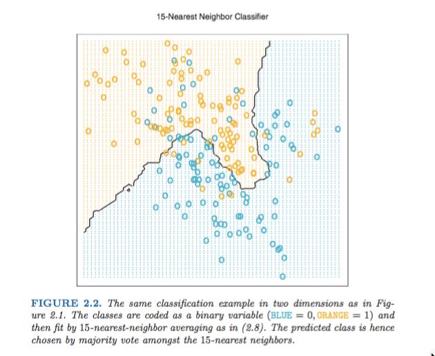
6 5/52

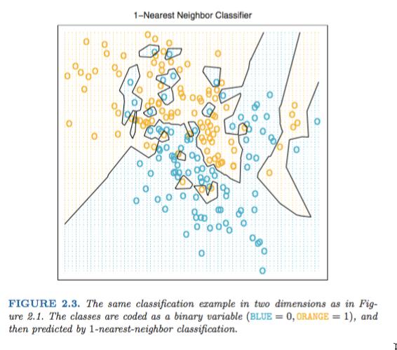
7 6/52

8 Higherdimensionalproblems, cont. What happens if we try to do basis expansion for linear regression in higher dimensions? 7/52

9 Higherdimensionalproblems, cont. What happens if we try to do basis expansion for linear regression in higher dimensions? For clarity, let s assume we just have two dimensions labeled x and z. We need a basis that looks like: y i = m j=0 k=0 m β j+m k x j i zk i + ϵ i So the number of coordinates grows to m 2 coefficients in order to fit arbitrary m dimensional polynomials. 7/52

10 Higherdimensionalproblems, cont. What happens if we try to do basis expansion for linear regression in higher dimensions? For clarity, let s assume we just have two dimensions labeled x and z. We need a basis that looks like: y i = m j=0 k=0 m β j+m k x j i zk i + ϵ i So the number of coordinates grows to m 2 coefficients in order to fit arbitrary m dimensional polynomials. For p dimensions, we ll need a total m p coefficients; a quickly unfeasible task. Regularization and keeping m small can help, but still makes this task hard for anything that would approximate a reasonably complex non-linear surface. 7/52

11 Higherdimensionalproblems, cont. Lowess, local polynomial regression, can be fit in the same manor as the linear model in higher dimensions. We can fix the order of the polynomial to be m = 1 while still capturing global non-linearity; therefore we can still use this technique in higher dimensions. 8/52

12 Additivemodels One way to deal with the problem of basis expansion in higher dimensions is to assume that there are no interaction between the variables. This leads to a model such as: These are known as additive models. y i = g 1 (x i,1 ) + g 2 (x i,2 ) + + g p (x i,p ) + ϵ i 9/52

13 Additivemodels, cont. Notice that the additive model cannot be defined uniquely as we can add a constant to one of the g j ( ) functions and subtract the same constant from another function g k ( ). In order to remedy this, one usually instead writes an explicit intercept term: y i = α + g 1 (x i,1 ) + g 2 (x i,2 ) + + g p (x i,p ) + ϵ i And constrains: g k (x i,k ) = 0 k For all values of k. 10/52

14 ComputingAdditivemodels The primary algorithm used for computing additive models is called the backfitting algorithm. It was originally used for additive models by Leo Breiman and Jerome Friedman: Breiman, Leo, and Jerome H. Friedman. Estimating optimal transformations for multiple regression and correlation. Journal of the American statistical Association (1985): /52

15 ComputingAdditivemodels, cont. The algorithm can be compactly described as: Data: pairs of data {(X i, y i )} n i=1 Result: Estimates α and ĝ j, j = {1, 2,..., p} i y i, ĝ j = 0 ; initialize α = 1 n while not converged do for j=1 to p do end end r ij y i â k j ĝk(x ik ) ĝ j S ( {(x ij, r ij )} n ) i=1 ĝ j ĝ j 1 n i ĝj(x ij ) For some smoother function S and stopping criterion. 12/52

16 ComputingAdditivemodels, cont. For the smoothing function S, we can use any of the algorithms we have already studied. Local polynomial regression is a popular choice. 13/52

17 ComputingAdditivemodels, cont. For the smoothing function S, we can use any of the algorithms we have already studied. Local polynomial regression is a popular choice. Notice that we can also blend the additive model with higher dimensional smoothers, particularly if we know that a small set of variables may have interactions with each other even though most variables do not: y i = α + g 1 (x i,1, x i,2 ) + g 3 (x i,3 ) + + g p (x i,p ) + ϵ i. 13/52

18 ComputingAdditivemodels, cont. There are two popular R packages for fitting additive models. Either mgcv: Or gam: /52

19 ComputingAdditivemodels, cont. There are two popular R packages for fitting additive models. Either mgcv: Or gam: There are not as many options for python. The best I know of is in statsmodels.sandbox.gam as AdditiveModel. 14/52

20 What swrongwithlinearregression? At this point you may wonder why linear regression seems to have trouble in higher dimensions compared to the local methods. In truth, all of these techniques have trouble with high dimensional spaces; it is just that the others hide this fact in their definitions. 15/52

21 What swrongwithlinearregression? At this point you may wonder why linear regression seems to have trouble in higher dimensions compared to the local methods. In truth, all of these techniques have trouble with high dimensional spaces; it is just that the others hide this fact in their definitions. The problem is the curse of dimensionality: When we have high dimensional spaces, datasets look sparse even when the number of samples is very large. 15/52

22 What swrongwithlinearregression? At this point you may wonder why linear regression seems to have trouble in higher dimensions compared to the local methods. In truth, all of these techniques have trouble with high dimensional spaces; it is just that the others hide this fact in their definitions. The problem is the curse of dimensionality: When we have high dimensional spaces, datasets look sparse even when the number of samples is very large. Dealing with this is going to be the motivating problem in machine learning for the remainder of the course. 15/52

23 Data analysis 16/52

24 Description Today we are going to look at housing price data, taking from the American Community Survey and prepared by Cosma Shalizi: The data list aggregate statistics for census tracts. 17/52

25 Let s first read in the data and look at all of the available variables. > x <- read.csv("data/capa.csv", as.is=true) > names(x) <- tolower(names(x)) > str(x) 'data.frame': obs. of 34 variables: $ x : int $ geo.id2 : num 6e+09 6e+09 6e+09 6e+09 6e $ statefp : int $ countyfp : int $ tractce : int $ population : int $ latitude : num $ longitude : num $ geo.display.label : chr "Census Tract 4001, Alameda County, California"... $ median_house_value : int NA $ total_units : int $ vacant_units : int $ median_rooms : num /52

26 $ mean_household_size_owners : num $ mean_household_size_renters: num $ built_2005_or_later : num $ built_2000_to_2004 : num $ built_1990s : num $ built_1980s : num $ built_1970s : num $ built_1960s : num $ built_1950s : num $ built_1940s : num $ built_1939_or_earlier : num $ bedrooms_0 : num $ bedrooms_1 : num $ bedrooms_2 : num $ bedrooms_3 : num $ bedrooms_4 : num $ bedrooms_5_or_more : num $ owners : num $ renters : num $ median_household_income : int $ mean_household_income : int /52

27 There are a few bad rows of data, but we can safely clean them out: > badrows <- (apply(is.na(x),1,sum)!= 0) > table(badrows) badrows FALSE TRUE > tapply(x$median_household_income, badrows, median, na.rm=true) FALSE TRUE > tapply(x$median_house_value, badrows, median, na.rm=true) FALSE TRUE > tapply(x$vacant_units, badrows, median, na.rm=true) FALSE TRUE > x <- na.omit(x) 20/52

28 As you may have guessed from the file name, the housing prices cover two distinct regions: > plot(x$longitude, x$latitude, pch=19, cex=0.5) 21/52

29 x$latitude x$longitude 22/52

30 Let s split these two states up into two separate datasets. I ll use the California set to start, but hopefully we will have time to go back to the Pennsylvania set. > ca <- x[x$statefp==6,] > pa <- x[x$statefp==42,] 23/52

31 As a warm-up to additive models, let s fit and tune simple knn model for whether the majority of residents in a census tract. > testflag <- (runif(nrow(ca)) > 0.8) > trainflag <-!testflag > cl <- as.numeric(ca$owners < 50) For the training set, we will use cross-validation to select the optimal k: > X <- cbind(ca$latitude,ca$longitude)[trainflag,] > y <- cl[trainflag] > foldid <- sample(1:5, nrow(x),replace=true) 24/52

32 Here is the main validation code, using misclassification error: > kvals <- 1:25 > res <- matrix(ncol=5, nrow=25) > for (i in 1:5) { + trainset <- which(foldid!= i) + validset <- which(foldid == i) + for (k in 1:25) { + pred <- knn(x[trainset,],x[validset,],y[trainset], + k=kvals[k]) + yhat <- (as.numeric(pred) - 1) + res[k,i] <- mean((y[validset]!= yhat)) + print(k) + } + } 25/52

33 Taking the results for each fold, I can calculate the cross validated mis-classification rate as well as the standard errors of these rates: > head(res) [,1] [,2] [,3] [,4] [,5] [1,] [2,] [3,] [4,] [5,] [6,] > cverror <- apply(res,1,mean) > cvse <- apply(res,1,sd) / sqrt(5) 26/52

34 cverror :25 27/52

35 If we set the tuning parameter to 4, we can then check how well this performs on the test set. > Xtest <- cbind(ca$latitude,ca$longitude)[testflag,] > ytest <- cl[testflag] > yhat <- (as.numeric(knn(x,xtest,y,k=4)) - 1) > mean((yhat!= ytest)) [1] 0.22 > round(table(yhat, ytest) / length(yhat) * 100) ytest yhat The table at the bottom is called a confusion matrix, and gives more granularity than the raw misclassification rate. 28/52

36 If we set the tuning parameter to 4, we can then check how well this performs on the test set. > Xtest <- cbind(ca$latitude,ca$longitude)[testflag,] > ytest <- cl[testflag] > yhat <- (as.numeric(knn(x,xtest,y,k=4)) - 1) > mean((yhat!= ytest)) [1] 0.22 > round(table(yhat, ytest) / length(yhat) * 100) ytest yhat The table at the bottom is called a confusion matrix, and gives more granularity than the raw misclassification rate. 29/52

37 Now, I want to understand the variables that effect the median house value in a census tract. Here is a linear model that would be a good starting point (after some exploratory plots, preferably): > ca.lm <- lm(log(median_house_value) ~ median_household_income + + mean_household_income + population + total_units vacant_units + owners + median_rooms mean_household_size_owners + mean_household_size_renters + + latitude + longitude, data = ca, subset=trainflag) 30/52

38 > summary(ca.lm) Estimate Std. Error t value Pr(> t ) (Intercept) -5.78e e < 2e-16 *** median_household_income 1.20e e * mean_household_income 1.08e e < 2e-16 *** population -4.15e e e-13 *** total_units 8.37e e e-06 *** vacant_units -1.06e e owners -3.83e e < 2e-16 *** median_rooms -1.49e e mean_household_size_owners 5.40e e e-11 *** mean_household_size_renters -7.46e e < 2e-16 *** latitude -2.15e e < 2e-16 *** longitude -2.15e e < 2e-16 *** --- Signif. codes: 0 *** ** 0.01 * Residual standard error: 0.32 on 5995 degrees of freedom Multiple R-squared: 0.636, Adjusted R-squared: F-statistic: 953 on 11 and 5995 DF, p-value: <2e-16 31/52

39 To fit an additive model in R, we can use the mgcv package. It uses cross-validation by default, making it very easy to use in place of linear regression. > library(mgcv) Loading required package: nlme This is mgcv For overview type 'help("mgcv -package")'. > ca.gam <- gam(log(median_house_value) + ~ s(median_household_income) + s(mean_household_income) + + s(population) + s(total_units) + s(vacant_units) + + s(owners) + s(median_rooms) + s(mean_household_size_owners) + + s(mean_household_size_renters) + s(latitude) + + s(longitude), data=ca, subset=trainflag) 32/52

40 To see the coefficients in the additive model, we can plot the output object. These options work well when working locally: > plot(ca.gam2,scale=0,se=2,shade=true,resid=false,pages=1) For class, I add the option select=i to only show the contribution of the i th variable. 33/52

41 s(median_household_income,4.9) median_household_income 34/52

42 s(mean_household_income,6.16) mean_household_income 35/52

43 s(population,1.88) population 36/52

44 s(total_units,4.21) total_units 37/52

45 s(vacant_units,5.95) vacant_units 38/52

46 s(owners,3.87) owners 39/52

47 s(median_rooms,7.73) median_rooms 40/52

48 s(mean_household_size_owners,7.66) mean_household_size_owners 41/52

49 s(mean_household_size_renters,2.03) mean_household_size_renters 42/52

50 s(latitude,8.86) latitude 43/52

51 s(longitude,8.88) longitude 44/52

52 It actually makes more sense to allow and interaction between latitude and longitude. This is also easy to include in mgcv: > ca.gam2 <- gam(log(median_house_value) + ~ s(median_household_income) + s(mean_household_income) + + s(population) + s(total_units) + s(vacant_units) + + s(owners) + s(median_rooms) + s(mean_household_size_owners) + + s(mean_household_size_renters) + + s(longitude,latitude), data=ca, subset=trainflag) 45/52

53 /52

54 How well does these methods do in terms of prediction? We can predict using the predict function just as with linear models: > y <- log(ca$median_house_value) > ca.lm.pred <- predict(ca.lm, ca) > ca.gam.pred <- predict(ca.gam, ca) > ca.gam2.pred <- predict(ca.gam2, ca) And then check the mean squared error on both the training set and testing set: > tapply((ca.lm.pred - y)^2, trainflag, mean) FALSE TRUE > tapply((ca.gam.pred - y)^2, trainflag, mean) FALSE TRUE > tapply((ca.gam2.pred - y)^2, trainflag, mean) FALSE TRUE /52

55 In machine learning, you ll often hear the caveat that everything depend on future values following the same underlying model. I think we say that a lot, but forget to really think about it. To illustrate, let s re-fit the model on the California data without the latitude and longitude components. We can then see how well the model trained on California data generalizes to Pennsylvania data. 48/52

56 Here are the two linear models fit on the two different datasets. > ca.lm2 <- lm(log(median_house_value) ~ median_household_income + + mean_household_income + population + total_units vacant_units + owners + median_rooms mean_household_size_owners + mean_household_size_renters, + data = ca, subset=trainflag) > > pa.lm3 <- lm(log(median_house_value) ~ median_household_income + + mean_household_income + population + total_units vacant_units + owners + median_rooms mean_household_size_owners + mean_household_size_renters, + data = pa, subset=trainflag) 49/52

57 And here are the two additive models fit on the data: > ca.gam3 <- gam(log(median_house_value) + ~ s(median_household_income) + s(mean_household_income) + + s(population) + s(total_units) + s(vacant_units) + + s(owners) + s(median_rooms) + s(mean_household_size_owners) + + s(mean_household_size_renters), data=ca, subset=trainflagpa) > > pa.gam4 <- gam(log(median_house_value) + ~ s(median_household_income) + s(mean_household_income) + + s(population) + s(total_units) + s(vacant_units) + + s(owners) + s(median_rooms) + s(mean_household_size_owners) + + s(mean_household_size_renters), data=pa, subset=trainflagpa) 50/52

58 Fitting these models all on the PA data: > y.pa <- log(pa$median_house_value) > pa.lm2.pred <- predict(ca.lm2, pa) > pa.gam3.pred <- predict(ca.gam3, pa) > pa.lm3.pred <- predict(pa.lm3, pa) > pa.gam4.pred <- predict(pa.gam4, pa) We see that the California ones yield very poor MSE scores for PA: > tapply((pa.lm2.pred - y.pa)^2,trainflagpa,mean) FALSE TRUE > tapply((pa.gam3.pred - y.pa)^2,trainflagpa,mean) FALSE TRUE > tapply((pa.lm3.pred - y.pa)^2,trainflagpa,mean) FALSE TRUE > tapply((pa.gam4.pred - y.pa)^2,trainflagpa,mean) FALSE TRUE /52

59 If we account for the overall means being different, we see that the California models perform reasonably well on the Pennsylvania data: > tapply((pa.lm2.pred - y.pa),trainflagpa,var) FALSE TRUE > tapply((pa.gam3.pred - y.pa),trainflagpa,var) FALSE TRUE > tapply((pa.lm3.pred - y.pa),trainflagpa,var) FALSE TRUE > tapply((pa.gam4.pred - y.pa),trainflagpa,var) FALSE TRUE /52