TV-L1 Optical Flow Estimation
|
|
|
- Jason Johns
- 6 years ago
- Views:
Transcription
1 214/7/1 v.5 IPOL article class Published in Image Processing On Line on Submitted on , accepted on ISSN c 213 IPOL & the authors CC BY NC SA This article is available online with supplementary materials, software, datasets and online demo at TV-L1 Optical Flow Estimation Javier Sánchez 1, Enric Meinhardt-Llopis 2, Gabriele Facciolo 3 1 CTIM, Universidad de Las Palmas de Gran Canaria, Spain (jsanchez@dis.ulpgc.es) 2 CMLA, ENS Cachan, France (enric.meinhardt@cmla.ens-cachan.fr) 3 CMLA, ENS Cachan, France (gabriele.facciolo@cmla.ens-cachan.fr) Abstract This article describes an implementation of the optical flow estimation method introduced by Zach, Pock and Bischof in 27. This method is based on the minimization of a functional containing a data term using the L 1 norm and a regularization term using the total variation of the flow. The main feature of this formulation is that it allows discontinuities in the flow field, while being more robust to noise than the classical approach by Horn and Schunck. The algorithm is an efficient numerical scheme, which solves a relaxed version of the problem by alternate minimization. Source Code A C implementation of this algorithm is provided. The source code and an online demo are accessible at the web page of this article 1. Keywords: optical flow, total variation 1 Introduction The method described in Zach, Pock and Bischof s article [6] is based on the brightness constancy assumption. Let I(x, y, t) be a video sequence, and let (x(t), y(t)) be the trajectory of a point in the image plane, then the brightness constancy assumption states that I(x(t), y(t), t) is constant: Applying the chain rule, d I(x(t), y(t), t) =. (1) dt I (ẋ, ẏ) + I =. (2) t This last identity must hold for the trajectories of every point in the image domain, whose velocities at one instant define a vector field u(x, y) = (u 1 (x, y), u 2 (x, y)). Thus, the vector field 1 Javier Sánchez, Enric Meinhardt-Llopis, Gabriele Facciolo, TV-L1 Optical Flow Estimation, Image Processing On Line, 3 (213), pp
2 Javier Sánchez, Enric Meinhardt-Llopis, Gabriele Facciolo u(x, y) satisfies pointwise the following linear condition, called the optical flow constraint equation [2]: I u + I =. (3) t For every point in the image domain, the condition I u + I = is a linear equation in two t variables (the components of u). Thus, there are altogether twice as many variables as equations, and the resulting linear system is underdetermined. A standard way to solve underdetermined systems is to add a smoothness condition, that forces u to be regular in some sense. The proposal of Horn and Schunck [2] was to select the u that minimizes the following functional: E Horn Schunck (u) = Ω ( I u + t I ) 2 + α ( u u 2 2). (4) This minimization problem is easy to solve by standard methods, and the resulting flow estimations are good enough for many purposes. The main shortcoming of the u u 2 2 term is that it penalizes high gradients of u and it effectively disallows discontinuities. Equation (3) is suitable if the image data is continuous in time. Typically, this equation is replaced by the non-linear formulation, I 1 (x + u) I (x) =, to account for general image sequences. The non-linear term I 1 (x + u) can be linearized using Taylor expansions, yielding the following equation: ρ(u) = I 1 (x + u ) (u u ) + I 1 (x + u ) I (x) =, (5) with u a close approximation to u. The Horn Schunck functional can be modified to allow discontinuities in the flow field by changing the quadratic factors, and this results in the method described here. The proposed algorithm can be understood as a minimization of the following energy functional, which is the sum of the total variation of u and an L 1 attachment term: E(u) = u 1 + u 2 + λ ρ(u). (6) Ω An efficient way to minimize this energy functional is to introduce the following convex relaxation: E θ (u, v) = u 1 + u θ u v 2 + λ ρ(v). (7) Ω Setting θ to a very small value forces the minimum of E θ to occur when u and v are nearly equal, reducing to the original energy E, defined in equation (6). The interest of this relaxation is that E θ can be minimized by alternatively fixing one of u or v, and solving for the other variable. 1. Fixed v, solve 2. Fixed u, solve min u 1 + u 2 + u Ω 1 2θ u v 2. (8) min v Ω 1 2θ u v 2 + λ ρ(v). (9) The first sub-problem fits the total variation denoising model of Rudin Osher Fatemi [4], which can be solved by Chambolle s duality-based algorithm [1]. The second sub-problem does not depend on spatial derivatives of v, so it can be solved point-wise by thresholding. 138
3 TV-L1 Optical Flow Estimation 2 Numerical Scheme The solution to the first minimization problem stated above can be obtained by computing the fixed point of the following iteration over the dual vector fields p 1 and p 2 : d := pk d + τ/θ ( v k+1 d + θdiv(p k d )) 1 + τ/θ ( v k+1 d + θdiv(p k d )), d {1, 2}, (1) p k+1 and recovering u as u k+1 d := v k+1 d + θdiv(p k d), d {1, 2}. (11) The second minimization problem can be solved as follows: v k+1 := u k+1 + T H(u k+1, u ), (12) with the thresholding operation λθ I 1 (x + u ) ifρ(u, u ) < λθ I 1 (x + u ) 2 T H(u, u ) := λθ I 1 (x + u ) ifρ(u, u ) > λθ I 1 (x + u ) 2. (13) ρ(u, u ) I 1(x+u ) if ρ(u, u ) λθ I I 1 (x+u ) 2 1 (x + u ) 2 This thresholding operation includes the information of the attachment term. When the objects move beyond the image limits, it is not possible to compute ρ, and it is convenient to disable this thresholding. Over these points, it is better to use only the regularization term. The input of the algorithm is a pair of images I (x) and I 1 (x), with x = (i, j) the pixel index. The output is a vector field u(x) = (u 1 (x), u 2 (x)). Note that the residual, ρ(u), is a scalar field (i.e., a gray-valued image), and its computation involves a warping of I 1 and I 1 by the deformation u. The vector field u must be close to u, so that the approximation error of the Taylor expansions above is small. The approximation field u is effectively computed by a multiscale scheme. 2.1 Numerical Details There are some numerical issues to be taken into account when implementing the algorithm. For example, it is essential for the difference schemes used to compute the divergence and the gradient to be adjoint linear operators, so that the Stokes theorem holds exactly. Here are the precise choices for this algorithm, for an image of size (N x, N y ): To compute the gradient of the image I 1, we use central differences along each direction, with Neumann boundary conditions. { I1 (i+1,j) I 1 (i 1,j) x I if1 < i < N 2 x 1(i, j) =, otherwise y I 1(i, j) = { I1 (i,j+1) I 1 (i,j 1) if1 < j < N 2 y. (14) otherwise To compute the gradient of each component of the flow u, we use forward differences with Neumann boundary conditions. { u(i + 1, j) u(i, j) if1 i < N x u(i, j) =, x ifi = N x u(i, j) = y { u(i, j + 1) u(i, j) if1 j < N y. (15) ifj = N y 139
4 Javier Sánchez, Enric Meinhardt-Llopis, Gabriele Facciolo For computing the divergences of the dual variables p, we use the adjoint of the gradient of u, which corresponds to using backward differences: p 1 (i, j) p 1 (i 1, j) if1 < i < N x div(p)(i, j) = p 1 (i, j) ifi = 1 p 1 (i 1, j) ifi = N x p 2 (i, j) p 2 (i, j 1) if1 < j < N y + p 2 (i, j) ifj = 1. (16) p 2 (i, j 1) ifj = N y To warp the image I 1 by a flow field u, we evaluate I 1 (x + u (x)) using bicubic interpolation. 3 Algorithm The algorithm that implements the method can be separated in two modules: a procedure that calculates the optical flow at a given scale, using the above numerical scheme; and a main algorithm that implements the pyramidal scheme and calls the procedure to obtain approximate solutions. The procedure updates a vector field u and uses three temporary vector fields v, p 1 and p 2, to perform intermediate computations. The initial value u of u is given by the enclosing multiscale procedure, and it is zero at the coarsest level. In order to stop the algorithm before the default number of iterations (N maxiter ), we use a stopping criterion based on the L 2 distance between consecutive values of u. When this distance is smaller than a given threshold, we assume that the algorithm has already converged. If u k, u k+1 are successive values of u, the stopping criterion is 1 ( u k+1 1 (i, j) u k N x N 1(i, j) ) 2 ( + u k+1 2 (i, j) u k 2(i, j) ) 2 < ε 2 y i,j (17) The procedure detects small displacements, but it fails when the correct magnitude of u is larger than about one pixel (depending on the smoothness of the image). In practice, to detect displacements larger than one pixel, it is useful to work with downscaled versions of the input images, where the sought for displacements are small enough. Then, the large (and rough) displacements obtained at the downscaled level can be refined at the original scale. A standard way to organize this process is by means of a pyramid of scales: a set of downscaled versions of the input images. In order to create the pyramid of images, we follow the same strategy as in our article on Horn Schunck optical flow [3]. To downscale an image, it is first convolved with a Gaussian kernel and then sampled using bicubic interpolation. We use a downsampling factor, η (, 1), that allows for smoother transitions between the scales. The algorithm is first run at the coarsest level, and the result is used as starting point in the finer levels. Algorithm 1 handles this pyramidal structure and relies on the previous procedure to estimate the optical flows at different scales. An improved version of this algorithm is described in an article by Wedel et al. [5], which introduces two filtering steps: a preprocessing of the input images by a structure-texture decomposition; and a median filtering of the optical flow after the warping step, enhancing the regularity of the flow. 14
5 TV-L1 Optical Flow Estimation Algorithm 1: Pyramidal structure management Input: I, I 1, τ, λ, θ, ε, η, N maxiter, N warps, N scales Output: u 1 Normalize images between and Convolve the images with a Gaussian of σ =.8 3 Create the pyramid of images I s using η (with s =,..., N scales 1) 4 u Nscales 1 (, ) 5 for s N scales 1 to do 6 TV-L 1 optical flow(i, I 1, u, τ, λ, θ, ε, N maxiter, N warps ) 7 if s > then 8 u s 1 (x) := 2u s (x/η) 9 end end 1 Procedure TV-L 1 optical flow(i, I 1, u, τ, λ, θ, ε, N maxiter, N warps ) p 1 (, ) p 2 (, ) for w 1 to N warps do Compute I 1 (x + u (x)), I 1 (x + u (x)) using bicubic interpolation n while n < N maxiter and stopping criterion > ε do v T H(u, u ) u v + θdiv(p) p p+τ/θ u 1+τ/θ u n n + 1 end end 4 Explanation of the Parameters In this section we explain the parameters of the method and give reasonable default values. The algorithm depends on six parameters: time step (τ), data attachment weight (λ), tightness (θ), stopping criterion threshold (ε), downsampling factor (η), number of scales (N scales ), number of warps (N warps ). τ is the time step of the numerical scheme. Chambolle shows [1] that the numerical scheme converges for values of τ <.125. Empirically, its value can be set to.25 for a faster convergence. λ is the attachment parameter. This is the most relevant parameter, which determines the smoothness of the output. The smaller this parameter is, the smoother the solutions we obtain. It depends on the range of motions of the images, so its value should be adapted to each image sequence. θ is the tightness parameter. It serves as a link between the attachment and the regularization terms. In theory, it should have a small value in order to maintain both parts in correspondence. The method is stable for a large range of values of this parameter. 141

6 Javier Sánchez, Enric Meinhardt-Llopis, Gabriele Facciolo ε is the stopping criterion threshold used in the numerical scheme, which is a trade-off between precision and running time. A small value will yield more accurate solutions at the expense of a slower convergence. η is the downsampling factor. It is used to downscale the original images in order to create the pyramidal structure. Its value must be in the interval (, 1). N scales is used to create the pyramid of images. If the flow field is very small (about one pixel), it can be set to 1. Otherwise, it should be set so that (1/η) N 1 is larger than the expected size of the largest displacement. See our article on Horn Schunck optical flow [3] for further details on this and the η parameters. N warps represents the number of times that I 1 (x + u ) and I 1 (x + u ) are computed per scale. This is a parameter that assures the stability of the method. It also affects the running time, so it is a compromise between speed and accuracy. Table 1: Parameters of the method. Parameter Description Default value τ time step.25 λ data attachment weight.15 θ tightness.3 ε stopping threshold.1 η zoom factor.5 N scales number of scales 5 N warps number of warps 5 5 Examples Figures 2 and 3 show the optical flows for the Ettlinger Tor and the Rheinhafen sequences, respectively. These sequences can be found at The results obtained are similar to the results in Zach et al. [6]. In these examples we have used the following parameters: τ=.25, θ=.5, η =.5, ε=.1, 5 scales and 5 warpings. The algorithm is executed for three values of λ. Figure 1: Color scheme used to represent the orientation and magnitude of optical flows. The method detects the displacement of the objects in the Ettlinger Tor traffic scene. It also detects a regular background motion maybe due to a small displacement of the camera and the effect of noise. For small values of λ (λ=.3), the solution is smoother and the optical flow is 142


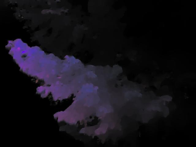
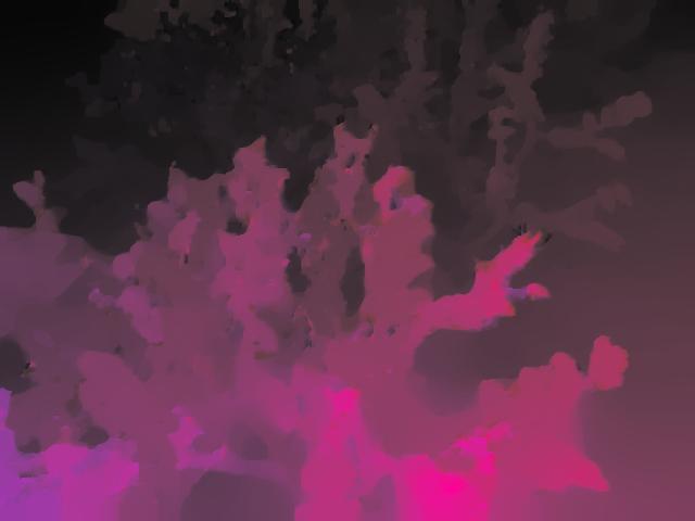
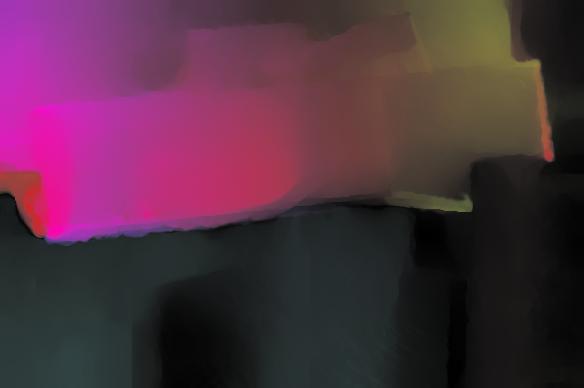
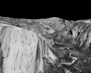
 we analyze the behavior for the the Yosemite sequences, both with and without clouds.")
![The flow is estimated between frames 8 and 9, as Zach et al. [6]. The parameters used for the sequence without clouds are τ =.25, λ=.11, θ=.45, η =.5, ε=.1, 5 scales and 5 warpings.](/docs-images/75/72744824/images/7-5.jpg "For the sequence with clouds the set of parameters are the same except for λ=.25 and θ =.6. The experiments in this section have been carried out in an Intel Core2 CPU at 2.")
. The results are slightly better than in Zach et al. [6].")
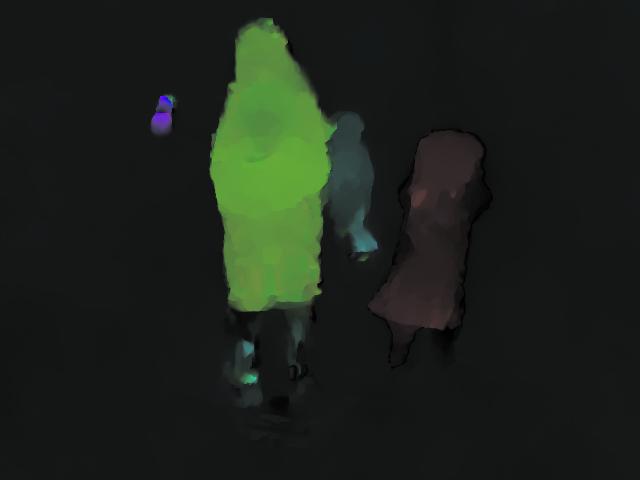
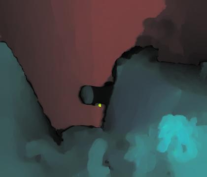
7 TV-L1 Optical Flow Estimation Ettlinger Tor λ =.2 λ =.3 λ = 1. Figure 2: Ettlinger Tor sequence. underestimated at the cars and the bus. Note that the method does not estimate the correct flow for the car next to the bus. When λ is big, the attachment term becomes more important and the method is more sensitive to the influence of noise, resulting in unstable flow fields. Rheinhafen λ =.2 λ =.3 λ = 1. Figure 3: Rheinhafen sequence. The results for the Rheinhafen sequence are similar: the method detects the movement of the cars and a small background shift. It also detects the motion of the shadow behind the truck. When λ is smaller, the flow fields are smoother and the effect of the shadow is spread. 5.1 Yosemite Sequence In this example (see figure 4) we analyze the behavior for the the Yosemite sequences, both with and without clouds. The flow is estimated between frames 8 and 9, as Zach et al. [6]. The parameters used for the sequence without clouds are τ =.25, λ=.11, θ=.45, η =.5, ε=.1, 5 scales and 5 warpings. For the sequence with clouds the set of parameters are the same except for λ=.25 and θ =.6. The experiments in this section have been carried out in an Intel Core2 CPU at 2.4 GHz with 2 GB of RAM. The source code uses OpenMP directives to parallelize several loops, but in the following examples, the running times are calculated for one processor only. In table 2, we show the Average End-Point Error and Average Angular Error (EPE and APE, respectively). The results are slightly better than in Zach et al. [6]. Note that our implementation uses several warpings per scale and a different stopping criterion, which depends on the convergence rate between intermediate solutions. The formulas used to calculate the EPE and AAE are: N q X u1,i ugt + u2,i ugt EP E := 1,i 2,i, N i=1 143 (18)


8 Javier Sánchez, Enric Meinhardt-Llopis, Gabriele Facciolo Figure 4: Yosemite and Yosemite with Clouds sequences. Table 2: EPE and AAE for the Yosemite test sequences. Errors EPE AAE Running time Yosemite.95 pixels 2.46 o 2.112s Yosemite with Clouds.251 pixels o 3.28s AAE := 1 N N u 1,i u gt 1,i arccos + u 2,iu gt 2,i, (19) i=1 u 21,i + u22,i + 1 u 2,gt 1,i + u 2,gt 2,i + 1 with u gt = (u gt 1, u gt 2 ) the ground truth solution. The running time may be further reduced if ε is increased and/or the number of warpings is decreased. In Zach et al. [6], the implementation and experiments were carried out with only one warping per scale. In figure 5 we observe the evolution of EPE and AAE with respect to θ, given several fixed values for λ. We observe that the errors decrease rapidly and then slowly increase. Note that, in order to appreciate the evolution of the error, the graphics are in logarithmic scale. From these graphics we observe that a value of θ =.3 is a good choice for several values of λ. 1 When θ is very large, the importance of the coupling term, u 2θ v 2, fades away and there is no effective transfer of information between u and v. When θ is very small, the coupling term outweighs the data and regularization terms at each iteration. Thus, there is too much transfer of information in the iterations and the solution is given by u = v. In either case (θ or θ ), the method provides bad results. In practice, there is a wide range of θ values for which the result is reasonable (e.g., between.1 and 1). Figure 6 shows the same error graphics changing the roles of λ and θ. A small value of λ creates very smooth flow fields since it increases the weight of the regularization. A larger value increases the dependency on the attachment term and the solutions become less regular. λ has a greater influence on the results and we observe that the solutions for λ.2 are more accurate. 144
9 TV-L1 Optical Flow Estimation Average End-Point Error Average Angular Error EPE in pixels λ =.1 λ =.5 λ =.1 λ =.2 λ =.3 AAE in degrees λ =.1 λ =.5 λ =.1 λ =.2 λ = θ θ Figure 5: Errors for sequence Yosemite with Clouds as a function of θ. Average End-Point Error Average Angular Error EPE in pixels θ =.1 θ =.2 θ =.5 θ =.1 θ =.5 θ = 1. AAE in degrees θ =.1 θ =.2 θ =.5 θ =.1 θ =.5 θ = λ λ Figure 6: Errors for sequence Yosemite with Clouds as a function of λ. 145
10 Javier Sánchez, Enric Meinhardt-Llopis, Gabriele Facciolo Table 3: EPE and AAE for the Middlebury test sequences, using default parameters. Errors Dimetrodon Grove2 Grove3 Hydrangea Rubberwhale Urban2 Urban3 Venus EPE.162p.156p.721p.258p.215p.382p.711p.394p AAE o o 6.59 o o o 3.16 o o o Table 4: EPE and AAE for the Middlebury test sequences, using the best parameters. Errors Dimetrodon Grove2 Grove3 Hydrangea Rubberwhale Urban2 Urban3 Venus EPE.152p.153p.673p.244p.199p.36p.535p.296p AAE o o o o o o o o 5.2 Middlebury Database This section shows several tests with the sequences in the Middlebury benchmark database 2. This database contains two types of data: those for which the ground truth are made public (called Test sequences ), and those for which the ground truth are not public ( Evaluation sequences ). The former are used for testing purposes and finding the appropriate parameters of the method, and the latter are used to develop a ranking on the web page Test Sequences For the test sequences, we have run the algorithm with the same parameter set: τ =.25, λ=.15, θ=.3, η =.5, ε=.1, 6 scales and 5 warpings. We also compute the optical flows adapting the values of λ, θ and the number of scales, in order to find a better result. Figure 7 shows the 1th frame of the sequence, the ground truth, the solution with fixed parameters and the best solution found. These sequences are composed of more than two frames, but the ground truth is only available for the 1th frame. Thus, the estimated optical flow is between frames 1 and 11. In table 3 we show the EPE and AAE for the Middlebury test sequences, when fixed parameters are used, which corresponds to the optical flows in the third column. In the fourth column of the figure, we show the best optical flows found and the parameters used. Table 4 shows the EPE and AAE for these experiments. In some cases, e.g. Urban3 and Venus, the improvements in accuracy are important. As in the previous section, we show the evolution of the EPE and AAE for λ and θ. In this case, we have used the RubberWhale sequence, which is a real video sequence with ground truth. In figure 8, we observe the evolution of EPE and AAE with respect to θ given several fixed values for λ. We observe again that the error evolution in θ is very stable. As it happened for the Yosemite sequence, values of θ around.3 seem to provide the best results. Figure 9 shows the same error graphics for λ and several fixed values of θ. In the case of RubberWhale, the best value for λ is around.3. In our experience, a value of λ =.15 yields good results for all the sequences Evaluation Sequences Finally, we show several examples using the evaluation sequences in figure 1. We have used the same parameter set as for the test sequences: τ=.25, λ=.15, θ=.3, η =.5, ε=.1, 6 scales and 5 warpings


11 TV-L1 Optical Flow Estimation Frame 1 Ground truth Optical flow Best optical flow Dimetrodon λ =.3 θ =.3 5 scales Grove2 λ =.3 θ =.3 6 scales Grove3 λ =.5 θ =.4 4 scales Hydrangea λ =.1 θ =.8 4 scales RubberWhale λ =.4 θ =.4 4 scales Urban2 λ =.5 θ =.3 6 scales Urban3 λ =.9 θ =.7 5 scales Venus λ =.4 θ =.6 4 scales Figure 7: Results for the Middlebury test sequences. 147
12 Javier Sánchez, Enric Meinhardt-Llopis, Gabriele Facciolo Average End-Point Error Average Angular Error EPE in pixels λ =.1 λ =.5 λ =.1 λ =.2 λ =.3 AAE in degrees λ =.1 λ =.5 λ =.1 λ =.2 λ = θ θ Figure 8: Errors for sequence RubberWhale as a function of θ. Average End-Point Error Average Angular Error EPE in pixels θ =.1 θ =.2 θ =.5 θ =.1 θ =.5 θ = 1. AAE in degrees θ =.1 θ =.2 θ =.5 θ =.1 θ =.5 θ = λ λ Figure 9: Errors for sequence RubberWhale as a function of λ. 148


13 TV-L1 Optical Flow Estimation Sequence Optical flow Sequence Figure 1: Middlebury evaluation sequences. 149 Optical flow
14 Javier Sa nchez, Enric Meinhardt-Llopis, Gabriele Facciolo Acknowledgements This work has been partly founded by the Spanish Ministry of Science and Innovation through the research project TIN , by the Centre National d Etudes Spatiales (CNES, MISS Project), by the European Research Council (advanced grant Twelve Labours) and by the Office of Naval research (ONR grant N ). Image Credits All images by the authors except: Standard test sequences, Henner Kollnig3. Standard test sequences, Lynn Quam4. Middlebury benchmark database5. References [1] Antonin Chambolle. An Algorithm for Total Variation Minimization and Applications. Journal of Mathematical Imaging and Vision, 2(1-2):89 97, January B:JMIV e [2] Berthold K. P. Horn and Brian G. Schunck. Determining optical flow : a retrospective. Artificial Intelligence, 17:185 23, [3] Enric Meinhardt-Llopis and Javier Sa nchez. Horn Schunck Optical Flow with a Multi-scale Strategy. Image Processing On Line, preprint, 212. [4] Leonid I. Rudin, Stanley Osher, and Emad Fatemi. Nonlinear total variation based noise removal algorithms. Physica D, 6: , November (92)9242-F [5] Andreas Wedel, Thomas Pock, Christopher Zach, Horst Bischof, and Daniel Cremers. Statistical and geometrical approaches to visual motion analysis. An Improved Algorithm for TV-L1 Optical Flow, pages Springer-Verlag, Berlin, Heidelberg, _2 [6] C. Zach, T. Pock, and H. Bischof. A Duality Based Approach for Realtime TV-L1 Optical Flow. In Fred A. Hamprecht, Christoph Schno rr, and Bernd Ja hne, editors, Pattern Recognition, volume 4713 of Lecture Notes in Computer Science, chapter 22, pages Springer Berlin Heidelberg, Berlin, Heidelberg,
Robust Optical Flow Estimation
 014/07/01 v0.5 IPOL article class Published in Image Processing On Line on 013 10 8. Submitted on 01 06, accepted on 013 05 31. ISSN 105 13 c 013 IPOL & the authors CC BY NC SA This article is available
Motion Estimation with Adaptive Regularization and Neighborhood Dependent Constraint
 0 Digital Image Computing: Techniques and Applications Motion Estimation with Adaptive Regularization and Neighborhood Dependent Constraint Muhammad Wasim Nawaz, Abdesselam Bouzerdoum, Son Lam Phung ICT
Notes 9: Optical Flow
 Course 049064: Variational Methods in Image Processing Notes 9: Optical Flow Guy Gilboa 1 Basic Model 1.1 Background Optical flow is a fundamental problem in computer vision. The general goal is to find
Video Super Resolution using Duality Based TV-L 1 Optical Flow
 Video Super Resolution using Duality Based TV-L 1 Optical Flow Dennis Mitzel 1,2, Thomas Pock 3, Thomas Schoenemann 1 Daniel Cremers 1 1 Department of Computer Science University of Bonn, Germany 2 UMIC
Optical Flow Estimation with CUDA. Mikhail Smirnov
 Optical Flow Estimation with CUDA Mikhail Smirnov msmirnov@nvidia.com Document Change History Version Date Responsible Reason for Change Mikhail Smirnov Initial release Abstract Optical flow is the apparent
A Duality Based Algorithm for TV-L 1 -Optical-Flow Image Registration
 A Duality Based Algorithm for TV-L 1 -Optical-Flow Image Registration Thomas Pock 1, Martin Urschler 1, Christopher Zach 2, Reinhard Beichel 3, and Horst Bischof 1 1 Institute for Computer Graphics & Vision,
ATV-L1OpticalFlowMethod with Occlusion Detection
 ATV-L1OpticalFlowMethod with Occlusion Detection Coloma Ballester 1, Lluis Garrido 2, Vanel Lazcano 1, and Vicent Caselles 1 1 Dept Information and Communication Technologies, University Pompeu Fabra 2
Robust Optical Flow Computation Under Varying Illumination Using Rank Transform
 Sensors & Transducers Vol. 69 Issue 4 April 04 pp. 84-90 Sensors & Transducers 04 by IFSA Publishing S. L. http://www.sensorsportal.com Robust Optical Flow Computation Under Varying Illumination Using
CUDA GPGPU. Ivo Ihrke Tobias Ritschel Mario Fritz
 CUDA GPGPU Ivo Ihrke Tobias Ritschel Mario Fritz Today 3 Topics Intro to CUDA (NVIDIA slides) How is the GPU hardware organized? What is the programming model? Simple Kernels Hello World Gaussian Filtering
Part II: Modeling Aspects
 Yosemite test sequence Illumination changes Motion discontinuities Variational Optical Flow Estimation Part II: Modeling Aspects Discontinuity Di ti it preserving i smoothness th tterms Robust data terms
CS-465 Computer Vision
 CS-465 Computer Vision Nazar Khan PUCIT 9. Optic Flow Optic Flow Nazar Khan Computer Vision 2 / 25 Optic Flow Nazar Khan Computer Vision 3 / 25 Optic Flow Where does pixel (x, y) in frame z move to in
SURVEY OF LOCAL AND GLOBAL OPTICAL FLOW WITH COARSE TO FINE METHOD
 SURVEY OF LOCAL AND GLOBAL OPTICAL FLOW WITH COARSE TO FINE METHOD M.E-II, Department of Computer Engineering, PICT, Pune ABSTRACT: Optical flow as an image processing technique finds its applications
Solving Vision Tasks with variational methods on the GPU
 Solving Vision Tasks with variational methods on the GPU Horst Bischof Inst. f. Computer Graphics and Vision Graz University of Technology Joint work with Thomas Pock, Markus Unger, Arnold Irschara and
ILLUMINATION ROBUST OPTICAL FLOW ESTIMATION BY ILLUMINATION-CHROMATICITY DECOUPLING. Sungheon Park and Nojun Kwak
 ILLUMINATION ROBUST OPTICAL FLOW ESTIMATION BY ILLUMINATION-CHROMATICITY DECOUPLING Sungheon Park and Nojun Kwak Graduate School of Convergence Science and Technology, Seoul National University, Korea
Matching. Compare region of image to region of image. Today, simplest kind of matching. Intensities similar.
 Matching Compare region of image to region of image. We talked about this for stereo. Important for motion. Epipolar constraint unknown. But motion small. Recognition Find object in image. Recognize object.
Tracking and Structure from Motion
 Master s Thesis Winter Semester 2009/2010 Tracking and Structure from Motion Author: Andreas Weishaupt Supervisor: Prof. Pierre Vandergheynst Assistants: Luigi Bagnato Emmanuel D Angelo Signal Processing
Motion and Optical Flow. Slides from Ce Liu, Steve Seitz, Larry Zitnick, Ali Farhadi
 Motion and Optical Flow Slides from Ce Liu, Steve Seitz, Larry Zitnick, Ali Farhadi We live in a moving world Perceiving, understanding and predicting motion is an important part of our daily lives Motion
Motion. 1 Introduction. 2 Optical Flow. Sohaib A Khan. 2.1 Brightness Constancy Equation
 Motion Sohaib A Khan 1 Introduction So far, we have dealing with single images of a static scene taken by a fixed camera. Here we will deal with sequence of images taken at different time intervals. Motion
Chapter 2 Optical Flow Estimation
 Chapter 2 Optical Flow Estimation Abstract In this chapter we review the estimation of the two-dimensional apparent motion field of two consecutive images in an image sequence. This apparent motion field
Motion Estimation (II) Ce Liu Microsoft Research New England
 Ce Liu Microsoft Research New England") Motion Estimation (II) Ce Liu celiu@microsoft.com Microsoft Research New England Last time Motion perception Motion representation Parametric motion: Lucas-Kanade T I x du dv = I x I T x I y I x T I y
Motion Estimation (II) Ce Liu celiu@microsoft.com Microsoft Research New England Last time Motion perception Motion representation Parametric motion: Lucas-Kanade T I x du dv = I x I T x I y I x T I y
COMPUTER VISION > OPTICAL FLOW UTRECHT UNIVERSITY RONALD POPPE
 COMPUTER VISION 2017-2018 > OPTICAL FLOW UTRECHT UNIVERSITY RONALD POPPE OUTLINE Optical flow Lucas-Kanade Horn-Schunck Applications of optical flow Optical flow tracking Histograms of oriented flow Assignment
Optic Flow and Basics Towards Horn-Schunck 1
 Optic Flow and Basics Towards Horn-Schunck 1 Lecture 7 See Section 4.1 and Beginning of 4.2 in Reinhard Klette: Concise Computer Vision Springer-Verlag, London, 2014 1 See last slide for copyright information.
EE795: Computer Vision and Intelligent Systems
 EE795: Computer Vision and Intelligent Systems Spring 2012 TTh 17:30-18:45 FDH 204 Lecture 11 140311 http://www.ee.unlv.edu/~b1morris/ecg795/ 2 Outline Motion Analysis Motivation Differential Motion Optical
Improving Motion Estimation Using Image-Driven Functions and Hybrid Scheme
 Improving Motion Estimation Using Image-Driven Functions and Hybrid Scheme Duc Dung Nguyen and Jae Wook Jeon Department of Electrical and Computer Engineering, Sungkyunkwan University, Korea nddunga3@skku.edu,
A Duality Based Algorithm for TV-L 1 -Optical-Flow Image Registration
 A Duality Based Algorithm for TV-L 1 -Optical-Flow Image Registration Thomas Pock 1,MartinUrschler 1, Christopher Zach 2, Reinhard Beichel 3, and Horst Bischof 1 1 Institute for Computer Graphics & Vision,
CS 565 Computer Vision. Nazar Khan PUCIT Lectures 15 and 16: Optic Flow
 CS 565 Computer Vision Nazar Khan PUCIT Lectures 15 and 16: Optic Flow Introduction Basic Problem given: image sequence f(x, y, z), where (x, y) specifies the location and z denotes time wanted: displacement
International Journal of Advance Engineering and Research Development
 Scientific Journal of Impact Factor (SJIF): 4.72 International Journal of Advance Engineering and Research Development Volume 4, Issue 11, November -2017 e-issn (O): 2348-4470 p-issn (P): 2348-6406 Comparative
Illumination-robust variational optical flow based on cross-correlation
 Illumination-robust variational optical flow based on cross-correlation József Molnár 1 and Dmitry Chetverikov 2 1 Computer and Automation Research Institute Hungarian Academy of Sciences, Budapest, Hungary
Dense Image-based Motion Estimation Algorithms & Optical Flow
 Dense mage-based Motion Estimation Algorithms & Optical Flow Video A video is a sequence of frames captured at different times The video data is a function of v time (t) v space (x,y) ntroduction to motion
Motion Estimation. There are three main types (or applications) of motion estimation:
 of motion estimation:") Members: D91922016 朱威達 R93922010 林聖凱 R93922044 謝俊瑋 Motion Estimation There are three main types (or applications) of motion estimation: Parametric motion (image alignment) The main idea of parametric motion
Members: D91922016 朱威達 R93922010 林聖凱 R93922044 謝俊瑋 Motion Estimation There are three main types (or applications) of motion estimation: Parametric motion (image alignment) The main idea of parametric motion
LOCAL-GLOBAL OPTICAL FLOW FOR IMAGE REGISTRATION
 LOCAL-GLOBAL OPTICAL FLOW FOR IMAGE REGISTRATION Ammar Zayouna Richard Comley Daming Shi Middlesex University School of Engineering and Information Sciences Middlesex University, London NW4 4BT, UK A.Zayouna@mdx.ac.uk
Comparison between Motion Analysis and Stereo
 MOTION ESTIMATION The slides are from several sources through James Hays (Brown); Silvio Savarese (U. of Michigan); Octavia Camps (Northeastern); including their own slides. Comparison between Motion Analysis
Technion - Computer Science Department - Tehnical Report CIS
 Over-Parameterized Variational Optical Flow Tal Nir Alfred M. Bruckstein Ron Kimmel {taln, freddy, ron}@cs.technion.ac.il Department of Computer Science Technion Israel Institute of Technology Technion
EE795: Computer Vision and Intelligent Systems
 EE795: Computer Vision and Intelligent Systems Spring 2012 TTh 17:30-18:45 FDH 204 Lecture 14 130307 http://www.ee.unlv.edu/~b1morris/ecg795/ 2 Outline Review Stereo Dense Motion Estimation Translational
Variational Optical Flow from Alternate Exposure Images
 Variational Optical Flow from Alternate Exposure Images A. Sellent, M. Eisemann, B. Goldlücke, T. Pock, D. Cremers, M. Magnor TU Braunschweig, University Bonn, TU Graz Two Image Optical Flow Pinpoint sharp
Motion Estimation using Block Overlap Minimization
 Motion Estimation using Block Overlap Minimization Michael Santoro, Ghassan AlRegib, Yucel Altunbasak School of Electrical and Computer Engineering, Georgia Institute of Technology Atlanta, GA 30332 USA
CS 4495 Computer Vision Motion and Optic Flow
 CS 4495 Computer Vision Aaron Bobick School of Interactive Computing Administrivia PS4 is out, due Sunday Oct 27 th. All relevant lectures posted Details about Problem Set: You may *not* use built in Harris
Multiple Combined Constraints for Optical Flow Estimation
 Multiple Combined Constraints for Optical Flow Estimation Ahmed Fahad and Tim Morris School of Computer Science, The University of Manchester Manchester, M3 9PL, UK ahmed.fahad@postgrad.manchester.ac.uk,
Project Updates Short lecture Volumetric Modeling +2 papers
 Volumetric Modeling Schedule (tentative) Feb 20 Feb 27 Mar 5 Introduction Lecture: Geometry, Camera Model, Calibration Lecture: Features, Tracking/Matching Mar 12 Mar 19 Mar 26 Apr 2 Apr 9 Apr 16 Apr 23
CS6670: Computer Vision
 CS6670: Computer Vision Noah Snavely Lecture 19: Optical flow http://en.wikipedia.org/wiki/barberpole_illusion Readings Szeliski, Chapter 8.4-8.5 Announcements Project 2b due Tuesday, Nov 2 Please sign
Robust Trajectory-Space TV-L1 Optical Flow for Non-rigid Sequences
 Robust Trajectory-Space TV-L1 Optical Flow for Non-rigid Sequences Ravi Garg, Anastasios Roussos, and Lourdes Agapito Queen Mary University of London, Mile End Road, London E1 4NS, UK Abstract. This paper
Optical Flow-Based Motion Estimation. Thanks to Steve Seitz, Simon Baker, Takeo Kanade, and anyone else who helped develop these slides.
 Optical Flow-Based Motion Estimation Thanks to Steve Seitz, Simon Baker, Takeo Kanade, and anyone else who helped develop these slides. 1 Why estimate motion? We live in a 4-D world Wide applications Object
Optical Flow Estimation
 Optical Flow Estimation Goal: Introduction to image motion and 2D optical flow estimation. Motivation: Motion is a rich source of information about the world: segmentation surface structure from parallax
3D Computer Vision. Dense 3D Reconstruction II. Prof. Didier Stricker. Christiano Gava
 3D Computer Vision Dense 3D Reconstruction II Prof. Didier Stricker Christiano Gava Kaiserlautern University http://ags.cs.uni-kl.de/ DFKI Deutsches Forschungszentrum für Künstliche Intelligenz http://av.dfki.de
smooth coefficients H. Köstler, U. Rüde
 A robust multigrid solver for the optical flow problem with non- smooth coefficients H. Köstler, U. Rüde Overview Optical Flow Problem Data term and various regularizers A Robust Multigrid Solver Galerkin
High Accuracy Optical Flow Estimation Based on a Theory for Warping
 High Accuracy Optical Flow Estimation Based on a Theory for Warping Thomas Brox, Andrés Bruhn, Nils Papenberg, and Joachim Weickert Mathematical Image Analysis Group Faculty of Mathematics and Computer
Optical flow and depth from motion for omnidirectional images using a TV-L1 variational framework on graphs
 ICIP 2009 - Monday, November 9 Optical flow and depth from motion for omnidirectional images using a TV-L1 variational framework on graphs Luigi Bagnato Signal Processing Laboratory - EPFL Advisors: Prof.
Coarse to Over-Fine Optical Flow Estimation
 Coarse to Over-Fine Optical Flow Estimation Tomer Amiaz* Eyal Lubetzky Nahum Kiryati* *School of Electrical Engineering School of Computer Science Tel Aviv University Tel Aviv 69978, Israel September 11,
Optical Flow Estimation with Large Displacements: A Temporal Regularizer
 ISSN:1575-6807 D.L.: GC-1317-1999 INSTITUTO UNIVERSITARIO DE CIENCIAS Y TECNOLOGIAS CIBERNETICAS Optical Flow Estimation with Large Displacements: A Temporal Regularizer Agustin Salgado, Javier Sánchez.
Occlusion-Aware Video Registration for Highly Non-Rigid Objects Supplementary Material
 Occlusion-Aware Video Registration for Highly Non-Rigid Objects Supplementary Material Bertram Taetz 1,, Gabriele Bleser 1,, Vladislav Golyanik 1, and Didier Stricker 1, 1 German Research Center for Artificial
ELEC Dr Reji Mathew Electrical Engineering UNSW
 ELEC 4622 Dr Reji Mathew Electrical Engineering UNSW Review of Motion Modelling and Estimation Introduction to Motion Modelling & Estimation Forward Motion Backward Motion Block Motion Estimation Motion
Feature Tracking and Optical Flow
 Feature Tracking and Optical Flow Prof. D. Stricker Doz. G. Bleser Many slides adapted from James Hays, Derek Hoeim, Lana Lazebnik, Silvio Saverse, who 1 in turn adapted slides from Steve Seitz, Rick Szeliski,
Capturing, Modeling, Rendering 3D Structures
 Computer Vision Approach Capturing, Modeling, Rendering 3D Structures Calculate pixel correspondences and extract geometry Not robust Difficult to acquire illumination effects, e.g. specular highlights
Marcel Worring Intelligent Sensory Information Systems
 Marcel Worring worring@science.uva.nl Intelligent Sensory Information Systems University of Amsterdam Information and Communication Technology archives of documentaries, film, or training material, video
The 2D/3D Differential Optical Flow
 The 2D/3D Differential Optical Flow Prof. John Barron Dept. of Computer Science University of Western Ontario London, Ontario, Canada, N6A 5B7 Email: barron@csd.uwo.ca Phone: 519-661-2111 x86896 Canadian
Real-Time Dense and Accurate Parallel Optical Flow using CUDA
 Real-Time Dense and Accurate Parallel Optical Flow using CUDA Julien Marzat INRIA Rocquencourt - ENSEM Domaine de Voluceau BP 105, 78153 Le Chesnay Cedex, France julien.marzat@gmail.com Yann Dumortier
Comparison Between The Optical Flow Computational Techniques
 Comparison Between The Optical Flow Computational Techniques Sri Devi Thota #1, Kanaka Sunanda Vemulapalli* 2, Kartheek Chintalapati* 3, Phanindra Sai Srinivas Gudipudi* 4 # Associate Professor, Dept.
Optical Flow. Adriana Bocoi and Elena Pelican. 1. Introduction
 Proceedings of the Fifth Workshop on Mathematical Modelling of Environmental and Life Sciences Problems Constanţa, Romania, September, 200, pp. 5 5 Optical Flow Adriana Bocoi and Elena Pelican This paper
Comparison of stereo inspired optical flow estimation techniques
 Comparison of stereo inspired optical flow estimation techniques ABSTRACT The similarity of the correspondence problems in optical flow estimation and disparity estimation techniques enables methods to
Filter Flow: Supplemental Material
 Filter Flow: Supplemental Material Steven M. Seitz University of Washington Simon Baker Microsoft Research We include larger images and a number of additional results obtained using Filter Flow [5]. 1
Computer Vision I. Announcements. Fourier Tansform. Efficient Implementation. Edge and Corner Detection. CSE252A Lecture 13.
 Announcements Edge and Corner Detection HW3 assigned CSE252A Lecture 13 Efficient Implementation Both, the Box filter and the Gaussian filter are separable: First convolve each row of input image I with
Texture Sensitive Image Inpainting after Object Morphing
 Texture Sensitive Image Inpainting after Object Morphing Yin Chieh Liu and Yi-Leh Wu Department of Computer Science and Information Engineering National Taiwan University of Science and Technology, Taiwan
Feature Tracking and Optical Flow
 Feature Tracking and Optical Flow Prof. D. Stricker Doz. G. Bleser Many slides adapted from James Hays, Derek Hoeim, Lana Lazebnik, Silvio Saverse, who in turn adapted slides from Steve Seitz, Rick Szeliski,
Motion Compensated Frame Interpolation with a Symmetric Optical Flow Constraint
 Motion Compensated Frame Interpolation with a Symmetric Optical Flow Constraint Lars Lau Rakêt, Lars Roholm, Andrés Bruhn and Joachim Weickert Department of Computer Science, University of Copenhagen Universitetsparken
Level lines based disocclusion
 Level lines based disocclusion Simon Masnou Jean-Michel Morel CEREMADE CMLA Université Paris-IX Dauphine Ecole Normale Supérieure de Cachan 75775 Paris Cedex 16, France 94235 Cachan Cedex, France Abstract
Stereo Scene Flow for 3D Motion Analysis
 Stereo Scene Flow for 3D Motion Analysis Andreas Wedel Daniel Cremers Stereo Scene Flow for 3D Motion Analysis Dr. Andreas Wedel Group Research Daimler AG HPC 050 G023 Sindelfingen 71059 Germany andreas.wedel@daimler.com
TV-L 1 Optical Flow for Vector Valued Images
 TV-L 1 Optical Flow for Vector Valued Images Lars Lau Rakêt 1, Lars Roholm 2, Mads Nielsen 1, and François Lauze 1 1 Department of Computer Science, University of Copenhagen, Denmark {larslau, madsn, francois}@diku.dk
A Non-Linear Image Registration Scheme for Real-Time Liver Ultrasound Tracking using Normalized Gradient Fields
 A Non-Linear Image Registration Scheme for Real-Time Liver Ultrasound Tracking using Normalized Gradient Fields Lars König, Till Kipshagen and Jan Rühaak Fraunhofer MEVIS Project Group Image Registration,
Horn-Schunck and Lucas Kanade 1
 Horn-Schunck and Lucas Kanade 1 Lecture 8 See Sections 4.2 and 4.3 in Reinhard Klette: Concise Computer Vision Springer-Verlag, London, 2014 1 See last slide for copyright information. 1 / 40 Where We
Revisiting Lucas-Kanade and Horn-Schunck
 Revisiting Lucas-Kanade and Horn-Schunck Andry Maykol G. Pinto *1, A. Paulo Moreira 2, Paulo G. Costa 3, Miguel V. Correia 4 INESC TEC and Department of Electrical and Computer Engineering, Faculty of
Adaptive Multi-Stage 2D Image Motion Field Estimation
 Adaptive Multi-Stage 2D Image Motion Field Estimation Ulrich Neumann and Suya You Computer Science Department Integrated Media Systems Center University of Southern California, CA 90089-0781 ABSRAC his
Using Subspace Constraints to Improve Feature Tracking Presented by Bryan Poling. Based on work by Bryan Poling, Gilad Lerman, and Arthur Szlam
 Presented by Based on work by, Gilad Lerman, and Arthur Szlam What is Tracking? Broad Definition Tracking, or Object tracking, is a general term for following some thing through multiple frames of a video
Mariya Zhariy. Uttendorf Introduction to Optical Flow. Mariya Zhariy. Introduction. Determining. Optical Flow. Results. Motivation Definition
 to Constraint to Uttendorf 2005 Contents to Constraint 1 Contents to Constraint 1 2 Constraint Contents to Constraint 1 2 Constraint 3 Visual cranial reflex(vcr)(?) to Constraint Rapidly changing scene
Motion and Tracking. Andrea Torsello DAIS Università Ca Foscari via Torino 155, Mestre (VE)
") Motion and Tracking Andrea Torsello DAIS Università Ca Foscari via Torino 155, 30172 Mestre (VE) Motion Segmentation Segment the video into multiple coherently moving objects Motion and Perceptual Organization
Motion and Tracking Andrea Torsello DAIS Università Ca Foscari via Torino 155, 30172 Mestre (VE) Motion Segmentation Segment the video into multiple coherently moving objects Motion and Perceptual Organization
convolution shift invariant linear system Fourier Transform Aliasing and sampling scale representation edge detection corner detection
 COS 429: COMPUTER VISON Linear Filters and Edge Detection convolution shift invariant linear system Fourier Transform Aliasing and sampling scale representation edge detection corner detection Reading:
arxiv: v1 [cs.cv] 2 May 2016
![arxiv: v1 [cs.cv] 2 May 2016](/thumbs/86/93079061.jpg "arxiv: v1 [cs.cv] 2 May 2016") 16-811 Math Fundamentals for Robotics Comparison of Optimization Methods in Optical Flow Estimation Final Report, Fall 2015 arxiv:1605.00572v1 [cs.cv] 2 May 2016 Contents Noranart Vesdapunt Master of Computer
16-811 Math Fundamentals for Robotics Comparison of Optimization Methods in Optical Flow Estimation Final Report, Fall 2015 arxiv:1605.00572v1 [cs.cv] 2 May 2016 Contents Noranart Vesdapunt Master of Computer
VC 11/12 T11 Optical Flow
 VC 11/12 T11 Optical Flow Mestrado em Ciência de Computadores Mestrado Integrado em Engenharia de Redes e Sistemas Informáticos Miguel Tavares Coimbra Outline Optical Flow Constraint Equation Aperture
Colour Segmentation-based Computation of Dense Optical Flow with Application to Video Object Segmentation
 ÖGAI Journal 24/1 11 Colour Segmentation-based Computation of Dense Optical Flow with Application to Video Object Segmentation Michael Bleyer, Margrit Gelautz, Christoph Rhemann Vienna University of Technology
Bilevel Sparse Coding
 Adobe Research 345 Park Ave, San Jose, CA Mar 15, 2013 Outline 1 2 The learning model The learning algorithm 3 4 Sparse Modeling Many types of sensory data, e.g., images and audio, are in high-dimensional
Video Completion via Spatio-temporally Consistent Motion Inpainting
 Express Paper Video Completion via Spatio-temporally Consistent Motion Inpainting Menandro Roxas 1,a) Takaaki Shiratori 2,b) Katsushi Ikeuchi 1,c) Received: April 25, 2014, Accepted: May 19, 2014, Released:
Probabilistic Observation Models for Tracking Based on Optical Flow
 Probabilistic Observation Models for Tracking Based on Optical Flow Manuel J. Lucena 1,JoséM.Fuertes 1, Nicolas Perez de la Blanca 2, Antonio Garrido 2,andNicolás Ruiz 3 1 Departamento de Informatica,
On a first-order primal-dual algorithm
 On a first-order primal-dual algorithm Thomas Pock 1 and Antonin Chambolle 2 1 Institute for Computer Graphics and Vision, Graz University of Technology, 8010 Graz, Austria 2 Centre de Mathématiques Appliquées,
An Evaluation of Robust Cost Functions for RGB Direct Mapping
 An Evaluation of Robust Cost Functions for RGB Direct Mapping Alejo Concha and Javier Civera Abstract The so-called direct SLAM methods have shown an impressive performance in estimating a dense 3D reconstruction
Image denoising using TV-Stokes equation with an orientation-matching minimization
 Image denoising using TV-Stokes equation with an orientation-matching minimization Xue-Cheng Tai 1,2, Sofia Borok 1, and Jooyoung Hahn 1 1 Division of Mathematical Sciences, School of Physical Mathematical
A Novel Image Super-resolution Reconstruction Algorithm based on Modified Sparse Representation
 , pp.162-167 http://dx.doi.org/10.14257/astl.2016.138.33 A Novel Image Super-resolution Reconstruction Algorithm based on Modified Sparse Representation Liqiang Hu, Chaofeng He Shijiazhuang Tiedao University,
Global motion model based on B-spline wavelets: application to motion estimation and video indexing
 Global motion model based on B-spline wavelets: application to motion estimation and video indexing E. Bruno 1, D. Pellerin 1,2 Laboratoire des Images et des Signaux (LIS) 1 INPG, 46 Av. Félix Viallet,
SUMMARY: DISTINCTIVE IMAGE FEATURES FROM SCALE- INVARIANT KEYPOINTS
 SUMMARY: DISTINCTIVE IMAGE FEATURES FROM SCALE- INVARIANT KEYPOINTS Cognitive Robotics Original: David G. Lowe, 004 Summary: Coen van Leeuwen, s1460919 Abstract: This article presents a method to extract
Stereo Wrap + Motion. Computer Vision I. CSE252A Lecture 17
 Stereo Wrap + Motion CSE252A Lecture 17 Some Issues Ambiguity Window size Window shape Lighting Half occluded regions Problem of Occlusion Stereo Constraints CONSTRAINT BRIEF DESCRIPTION 1-D Epipolar Search
B. Tech. Project Second Stage Report on
 B. Tech. Project Second Stage Report on GPU Based Active Contours Submitted by Sumit Shekhar (05007028) Under the guidance of Prof Subhasis Chaudhuri Table of Contents 1. Introduction... 1 1.1 Graphic
Computer Vision I - Filtering and Feature detection
 Computer Vision I - Filtering and Feature detection Carsten Rother 30/10/2015 Computer Vision I: Basics of Image Processing Roadmap: Basics of Digital Image Processing Computer Vision I: Basics of Image
SIFT: SCALE INVARIANT FEATURE TRANSFORM SURF: SPEEDED UP ROBUST FEATURES BASHAR ALSADIK EOS DEPT. TOPMAP M13 3D GEOINFORMATION FROM IMAGES 2014
 SIFT: SCALE INVARIANT FEATURE TRANSFORM SURF: SPEEDED UP ROBUST FEATURES BASHAR ALSADIK EOS DEPT. TOPMAP M13 3D GEOINFORMATION FROM IMAGES 2014 SIFT SIFT: Scale Invariant Feature Transform; transform image
A MOTION MODEL BASED VIDEO STABILISATION ALGORITHM
 A MOTION MODEL BASED VIDEO STABILISATION ALGORITHM N. A. Tsoligkas, D. Xu, I. French and Y. Luo School of Science and Technology, University of Teesside, Middlesbrough, TS1 3BA, UK E-mails: tsoligas@teihal.gr,
Visualizing level lines and curvature in images
 Visualizing level lines and curvature in images Pascal Monasse 1 (joint work with Adina Ciomaga 2 and Jean-Michel Morel 2 ) 1 IMAGINE/LIGM, École des Ponts ParisTech/Univ. Paris Est, France 2 CMLA, ENS
A non-local algorithm for image denoising
 A non-local algorithm for image denoising Antoni Buades, Bartomeu Coll Dpt. Matemàtiques i Informàtica, UIB Ctra. Valldemossa Km. 7.5, 07122 Palma de Mallorca, Spain vdmiabc4@uib.es, tomeu.coll@uib.es
Computational Optical Imaging - Optique Numerique. -- Single and Multiple View Geometry, Stereo matching --
 Computational Optical Imaging - Optique Numerique -- Single and Multiple View Geometry, Stereo matching -- Autumn 2015 Ivo Ihrke with slides by Thorsten Thormaehlen Reminder: Feature Detection and Matching
What have we leaned so far?
 What have we leaned so far? Camera structure Eye structure Project 1: High Dynamic Range Imaging What have we learned so far? Image Filtering Image Warping Camera Projection Model Project 2: Panoramic
Local Feature Detectors
 Local Feature Detectors Selim Aksoy Department of Computer Engineering Bilkent University saksoy@cs.bilkent.edu.tr Slides adapted from Cordelia Schmid and David Lowe, CVPR 2003 Tutorial, Matthew Brown,
Computer Vision II Lecture 4
 Computer Vision II Lecture 4 Color based Tracking 29.04.2014 Bastian Leibe RWTH Aachen http://www.vision.rwth-aachen.de leibe@vision.rwth-aachen.de Course Outline Single-Object Tracking Background modeling
IMAGE FUSION WITH SIMULTANEOUS CARTOON AND TEXTURE DECOMPOSITION MAHDI DODANGEH, ISABEL NARRA FIGUEIREDO AND GIL GONÇALVES
 Pré-Publicações do Departamento de Matemática Universidade de Coimbra Preprint Number 15 14 IMAGE FUSION WITH SIMULTANEOUS CARTOON AND TEXTURE DECOMPOSITION MAHDI DODANGEH, ISABEL NARRA FIGUEIREDO AND
Lecture 16: Computer Vision
 CS4442/9542b: Artificial Intelligence II Prof. Olga Veksler Lecture 16: Computer Vision Motion Slides are from Steve Seitz (UW), David Jacobs (UMD) Outline Motion Estimation Motion Field Optical Flow Field