A workflow to account for uncertainty in well-log data in 3D geostatistical reservoir modeling

Transcription

1 A workflow to account for uncertainty in well-log data in 3D geostatistical reservoir Jose Akamine and Jef Caers May, 2007 Stanford Center for Reservoir Forecasting Abstract Traditionally well log data is used as hard data in reservoir using geostatistics; this means that we apply a constraint that needs to be honored exactly by the reservoir model. But if we know that a log is not reliable because of the log quality then the model will be constrained by non-reliable data. One could then argue in more general terms that in most practical cases hard data on either facies or petrophysical properties does not exist because well log data requires processing and interpretation before reaching the geostatistical stage. The traditional method approach using Kriging with error variance assumes that the reservoir modeler knows the error covariance and assumes it is uncorrelated. Another traditional approach, the Bayesian, assumes Gaussianity because the likelihood of the error model cannot be easily obtained. In order to overcome these limitations a data pre-posterior iterative algorithm approach is proposed. Several realizations of the uncertain well log data are generated taking into account the reliability of the well log measurements and they serve as input for the reservoir modeler to loosen the well constraints while at the same time honoring the geological spatial continuity. We present an application of this workflow to a real reservoir case study. 1 Introduction In stochastic, one aims at creating several realizations of some true spatial phenomenon. These realizations are constrained to a variety of data, typically categorized in hard data versus soft data. Soft data are data that provide indirect information about the primary variable under investigation. Soft data are measurements of a secondary variable that is related to the primary variable. Hard data are direct measurements of 1

2 the primary variable itself. These measurements are assumed to be exact (no error) and on the same support as the primary variable being modeled. In this text we focus on hard data, more specifically on the fact that in most practical application hard data are never truly hard. It is rare that we can get exact measurements, let alone on the same support as the variable being modeled. Various reasons exist: 1. A missing scale problem: the actual measurements are much smaller than the grid cell volume. Typically data taken from cored soil or rock samples are very small. It is not realistic, nor desired, to create a grid with unit grid-cell dimension the size of that small sample. Two solutions exist: (1) corner-point grid: simulate at the support of the core, but on a grid that is coarse (i.e. small support cells are located at the intersection of the grid vertices) or (2) cell-centered grid: perform an implicit upscaling by assuming that the core measurement is representative for the entire grid cell in which it is located. 2. A location problem: the exact position of the measurement is not known. 3. A data interpretation problem: even hard data are the result of some form of interpretation or calibration. For example well logs are used to interpret porosity or (lithological or depositional) facies variability along a well, then these porosity and facies data are used as hard data. Since interpretations are subjective, the data are not exact. 4. A measurement error problem: measurement devices create errors. The problem of uncertain hard data has been largely overlooked in stochastic or it has been treated using overly simplistic assumptions, for example by uncertainty as a simple error variance, often homoscedastic, or by calling for variogram models or likelihood functions that may not be easily assessed in real world situations. One should also note that in all rigor an uncertain hard datum is different from a soft datum. Soft data is a measurement of a secondary (another) variable, not of the primary variable. We often do not care about the spatial continuity of secondary variables (e.g. secondary variogram) as much as we care about the continuity of the primary variable. In co-simulation approaches, we do not aim at reproducing the secondary variogram; hence these techniques may not apply here. Therefore we prefer to use the term uncertain hard data although we acknowledge the contradiction in terms of such statement; it is intended to distinguish it from soft data Using the well log as hard data restricts the reservoir models in the well bore and the grids surrounding it in a reservoir model. However, several well log realizations 2

3 taking in consideration the uncertainty of the hard data and the spatial continuity will reduce the constraint in the reservoir models as shown in Figure 1. Figure 1: Traditional vs proposed approach In this paper, we review some proposed avenues to tackle this problem (Akamine and Caers (2006)), whether the primary variable is categorical or continuous and we present a workflow on how to use the proposed method to take into account uncertainty in well logs in a 3D reservoir with 15 wells. 2 Review of Traditional Methods Two approaches can be used to address the problem of well log uncertainty, each with its own limitations. 2.1 Kriging with error variance The kriging procedure can be used if the variable Z being modeled is continuous, then one can write the n hard data as in Equation (1). Z ɛ (u α ) = Z (u α ) + ɛ α α = 1,..., n (1) where Z (u α ) is the true unknown value of Z at u α, and ɛ α is the error made. Typically one assumes that the error has no bias, (zero expectation), it is uncorrelated 3

4 with Z, but errors may be correlated with each other, i.e. some variance/covariance model of the error exists as in Equation (2). E [ɛ α ɛ β ] = ercov αβ α, β = 1,..., n (2) The simple kriging estimator (zero mean case) is shown in Equation (3), Z (u) = n λ α (Z (u)) + ɛ α (3) α=1 and the kriging system is shown in Equation (4). n λ β (C (u β u α ) + ercov αβ ) = C (u u α ) (4) β=1 This kriging procedure can be implemented in sgsim (multi-gaussian Assumption) or dssim (no-multi-gaussian assumption), however dssim does not require a Gaussian tranform to change the variance of Z to unity neither assume that the variance of the error has the same transform. The limitation of this approach is that we assume that we know the error covariance ercov αβ and it will work only for continuous variables. 2.2 Bayesian In a Bayesian framework, the joint uncertainty of all variables Z (u), denoted as Z, is modeled using the posterior probability as in Equation (5). f (Z {Z ɛ (u α ), α = 1,..., n}) f (Z ɛ (u α ), α = 1,..., n Z) f (Z) (5) If the errors are assumed independent of the signal and of each other, then conditional independence applies and the posterior probability will be as in Equation (6). f (Z {Z ɛ (u α ), α = 1,..., n}) f (Z) And if no bias in the error is present, then: n f (Z ɛ (u α ) Z) (6) α=1 f (Z ɛ (u α ) Z) = f (ɛ) (7) In other words, the likelihood distribution is reduced to an error model. In a multi- Gaussian context, one assumes that all f are Gaussian, whether conditional, univariate or multi-variate. For the error model a Gaussian distribution with zero mean and error variance is used. Theoretically, in all generality, the Bayesian framework in Equation (7) does not require assumptions of multi-gaussianity or conditional independence. However, in 4

5 practice, this assumptions are often needed to make the methods practical, first from a sampling point of view, secondly because the data is not available to fully determine the likelihood distribution on Equation (7). The likelihood distribution expresses the joint uncertainty about the data for any possible reference field z. This would require one to know the exact forward model g that represents the link between the reference field and the data emanating from taking measurements from it as in Equation (8). {Z ɛ (u α ), α = 1,..., n} = g (Z) (8) In the case of errors of measurement devices, this may not be well-known. For example, we cannot possibly model the complete physics of a neutron-logging tool to predict what its response would be under certain field conditions. Moreover, in the case the error is due to interpretation it is not clear at all what the forward model is, then g is function of the (human) interpreter. A second limitation lies in the fact that these method also applies to continuos variables. 3 The Data Set The confidential well log data used in Section 4, Proposed Method, is introduced. The 15 wells belongs to a distal supra fan environment in a sub-marine delta depositional system. The oldest well was logged in 1976 and the newest was logged in The technology used ranges from a wireline triple-combo to logging while drilling technology (LWD). The reservoir has cells. The cell size is 120m 100m 2ft. In the reservoir portion of interest the 15 wells are mostly vertical. Figure 2 shows the well distribution in the Stanford Geostatistical Modeling Software (SGeMS). The horizontal separation between the wells did not allow the identification of a horizontal range less than 10 grid cells as seen in Figures 3(a) and 3(b), however in the vertical variogram in Figure 3(c) a range of 10 grid cells was identified. Although the reservoir models generated are constrained to two-point statistics only the multiplepoint code snesim was used using a sisim generated training image. The training image have vertical range of 10 and 3 horizontal (isotropic) range-cases: 10, 30 and Proposed Method The proposed method consists of three steps: 5

6 Figure 2: Well location in SGeMS (a) Y-direction (b) X-direction (c) Z-direction Figure 3: Variogram in the x, y and z direction 6

7 1. Create a pre-posterior probability that models the uncertainty of the hard data. Traditionally a hard data set is assigned to the grid in a reservoir model and those values are used as constraints to generate several realizations. In this proposal, hard data is not assigned to data location instead we assign a pre-posterior probability. In Figure 4(a) the traditional hard data representation of a binary variable is shown in a 2D reservoir while on Figure 4(b) an example of an uncertain hard data set is shown. (a) hard data (b) pre-posterior Figure 4: Hard data assigned to well locations (traditional approach) and data preposterior assigned to the well location (proposed approach) 2. Draw several hard data sets that honor the data pre-posterior and the geological continuity model. An iterative method is proposed such that all hard data locations are visited and the data pre-posterior is integrated with a given geological continuity constraint on the variable of interest. This method can be used for continuous variables and discrete variables and using two-point statistics and multiple-point statistics. 3. Generate multiple reservoir models with each hard data set, whether with a twopoint statistical or a multiple-point statistical method. The total set of models accounts for the geological continuity as well as the hard data uncertainty. Each step will now be discussed in more detail. 7

8 5 The data pre-posterior In most cases, one does not have access to likelihood distributions; instead it is more practical to assume that for each hard data location, one can provide a probability distribution describing the possible outcomes of hard data at that location as in Equation (9). f (Z ɛ (u α ) measurement at u α ) (9) In other words, given the results from a measurement device, one has either interpreted or calibrated the possible range of values and their frequencies. Note that Equation (9) does not require a forward model, it can be directly obtained from the measurements. We call Equation (9) a data pre-posterior, i.e. some prior information on the true value at u is available, however it is not yet a posterior distribution as other data sources are not yet accounted for (e.g. spatial continuity, other hard data, soft data, etc... ). We argue that working with data pre-posteriors is more practical than working with data likelihoods. Indeed, a data-pre-posterior could be obtained for the type of errors described in the introduction: 1. Missing scale: a fine-scale with unit-grid cell simulation of the spatial variable based on geological or other information could be done. Using many simulations, one could calculate Equation (9) empirically, i.e. tabulate frequency distribution of the entire grid-block property is for a given small-scale measurement. 2. Location: this problem could be handled similar as in the missing scale problem. 3. Interpretation: the interpreter could provide, based on his expertise, a distribution of values rather than a single interpretation. This distribution could be based on a confidence interval that he/she places on that single interpretation. 4. Measurement error: a simple Gaussian model with error variance could be used, or any other probability distribution for that matter. Note that the data pre-posterior concept also applies to discrete variables, where instead of a hard indicator datum, a probability can be provided expressing the uncertainty of the indicator event occurring: P r (I (u α ) = 1 measurement at u α ) (10) Following we present one workflow to obtain the data pre-posterior. 8

9 5.1 A workflow to obtain the data pre-posterior The workflow used to obtain the data pre-posterior from 15 wells using the Gamma Ray log curve is shown in Figure 5. The data pre-posterior for discrete variables in Equation (10) is equivalent in this case to the probability of having sand given the Gamma Ray log: P (A well log) where A is sand and the well log is the Gamma Ray log curve. The P (A well log) is obtained by a direct relationship to the shale volume content (V sh ). In the case of the Gamma Ray log the shale volume content (V sh ) can be linearly related to the shale index (I sh ) as in Equation (11), V sh = I sh = γ log γ clean γ shale γ clean (11) where γ log is the gamma ray response in the zone of interest obtained from the log, γ clean is the average gamma ray response in the cleanest formations and γ shale is the average gamma ray response in shales. The γ clean and γ shale are values that need to be chosen by the interpreter, therefore it can be considered as an additional source of uncertainty. Alternative non-linear correlations between V sh and I sh exists as explained in the following sub-sections. The existence of these alternatives is an additional source of scenario-based uncertainty. In the workflow, first we identify the sources of uncertainty that affects the Gamma Ray log. The 4 sources of uncertainties analyzed are: 1. Measurement Error 2. Gamma Ray shale pick 3. Gamma Ray clean pick 4. I sh to V sh Correlation curve selection 5. V sh sand / no sand cutoff Secondly, we construct a probability distribution function (pdf) that integrates these sources of uncertainties into a single model. Third, using Monte Carlo simulation we draw from the pdf and compare it to a V sh cutoff that differentiates sand from no-sand. The fraction of values that are drawn as sand will form the data preposterior: P (A well log). Each step will be explained in more detailed in the following sub-sections. 9

10 Figure 5: Workflow to obtain the data pre-posterior from the Gamma Ray log curve In this study, a group of 15 wells exists in the reservoir. To explain in detail the workflow to obtain the data pre-posterior we only use the Well A shown in Figure Measurement Error The well log is assumed to have a +/- 5% measurement error as a uniform distribution centered at the well log measurement value values are drawn from the uniform distribution probability function. A bias towards more certain sand is seen in Figure 11 because of a relative error of +/-5% is considered instead of an absolute error of +/-10 GAPI. This issue is still under research. Measurement errors will vary depending on several factors (i.e. technology used, the loggers technique, etc.). In this paper an arbitrary measurement error was applied depending on the year the well was logged, which is related to the technology used. The results are shown in Section Gamma Ray shale and Gamma Ray clean pick The gamma ray curve from the well log in Figure 6 is used. A cutoff for clean sand and shale is interpreted as shown in Figure 7. 10

11 Figure 6: Well Log A 11

12 Figure 7: Gamma Ray curve and cutoffs for clean sand and shales The values of GR lower than the GR clean cutoff are grouped to form a cumulative distribution function (cdf) of the GR clean in Figure 8(a) and similarly the values of GR higher than the GR shale cutoff are grouped as shown in Figure 8(b). (a) Clean GR (b) Shale GR Figure 8: Cumulative Distribution Function of the GR values By Monte Carlo Simulation, 1000 values are drawn from the lower quintile of the GR clean cdf. These values are then used as alternative γ clean values. Similarly 1000 values are drawn from the higher quintile of the GR shale cdf. The alternative values 12

13 are used as the γ clean and γ shale respectively in Equation (11) Gamma Ray Correlation Curve Generally a linear relation (V sh = I sh ) is used to calculate V sh from GR logs. However this can exaggerate the shale volume (Bassiouni (1994, p.312)) therefore other correlations between V sh and I sh could be used as alternatives such as the Larionov for tertiary rocks: the Stieber equation: the Clavier et al. equation: V sh = ( 2 3.7I sh 1 ), (12) V sh = I sh (3 2I sh ), (13) and for older rocks, the Larionov: V sh = 1.7 [ 3.38 (I sh + 0.7) 2] 1/2, (14) as shown in Figure 9. V sh = 0.33 ( 2 2I sh 1 ), (15) Figure 9: V sh vs I sh Correlation Curves 13

14 In addition to these correlations one can develop correlations specifically for a formation or geological unit of interest. We assign a probability of 60% for the linear interpretation to be an appropiate model; all other interpretations are assigned a 10% probability V sh sand / shale cutoff To differentiate between sand and shale a V sh cutoff is selected. In this workflow the V sh cutoff is considered also a source of uncertainty since it is also selected by the interpreter, therefore by Monte Carlo simulation 1000 values from a uniform probability distribution function between 0.4 and 0.6 are used as the V sh cutoff. 5.2 Probability Distribution Function From each value of Gamma Ray with the given measurement error at the specific depth and the 1000 drawings of GR shale and clean, a probability distribution function (pdf) of V sh is constructed by Monte Carlo simulation as shown in Figure 10. Values greater than one and lower than zero are rejected, since the definition of volume of shale content, V sh, is the volume of shale per unit volume of reservoir rock and it cannot be greater than the total volume of reservoir rock neither a negative value. Figure 10: Probability distribution function of V sh 14

15 Using Monte Carlo Simulation 1000 values for each depth are drawn from the V sh pdf and using the V sh sand / shale cutoff, the values are averaged to obtain P (A well log) as shown in Figure 11. The values of P (A well log) are used in the proposed algorithm as the data pre-posterior and the results are presented in the following sections. Figure 11: P (A well log) versus hard data 5.3 A workflow to obtain several discrete hard data sets that honor the data pre-posterior and the geological continuity Two-point statistics Traditionally, to integrate the pre-posterior probabilities one would opt for a co-indicator simulation approach. Consider the case of a binary indicator variable I (u), then the uncertainty of each unsampled value can be modeled using indicator kriging as in Equation (16): P r (I (u) = 1 data ) p = n λ α (P r (I (u α ) = 1 measurement at u α ) p) (16) α=1 If used in a sequential simulation context, there may be some additional previously simulated values that are treated as hard data. The kriging system in Equation (16) calls for the cross-variogram between the data pre-posterior probabilities and the primary variable. Inference of this cross-variogram may be problematic because, if all 15

16 hard data are uncertain, no direct observation of the primary variable is available, after all that is the premise here! A possible solution would be to create pseudo hard data by means of classification from the data pre-posterior, then infer primary and cross-variogram. However, such classification is done independently from one location to another, ignoring spatial continuity, moreover, since the hard data are obtained from the data pre-posterior, one may overestimate the dependency between the pre-posterior probabilities and primary variable. If a cross-variogram cannot be inferred, than this essentially means that the redundancy between the primary variable (in essence its spatial continuity) and the uncertain hard data cannot be accurately assessed. However, recall that the goal of spatial simulation is not primarily to assess data redundancy (i.e. model variogram and crossvariogram), but to create realizations that reflect some prior spatial continuity model and fit the data either exactly (hard) or to some extent (uncertain hard). Hence, we reverse the problem: assume we know the redundancy, then, for that given redundancy, does the resulting realization reflect the important properties we want to impose on them? In other words, we could by trail and error try various variogram models until we find one that does the job. However, since variogram models are tedious to handle (multiple parameters) and since the information given here is in terms of probabilities, a better alternative would be to frame the redundancy issue directly in terms of probabilities rather than work with variograms. Journel (2002) proposes a model (in terms of probabilities) that allows to decompose the problem of assessing the uncertainty about some unknown from different data sources, into a problem of assessing the information content of each data source on the unknown separately from assessing the redundancy of information between data sources. If D 1, D 2,..., D n data sources are available about some unknown A, then the posterior probability P (A D 1, D 2,..., D n ) can be assessed as in Equation (17): where: P (A D 1, D 2,..., D n ) = x [0, 1] (17) x x 0 = n i=1 ( xi x 0 ) τi (18) and the data probability ratios x 0, x 1,..., x n and the target ratio x, all valued in [0, ] as: x 0 = 1 P (A) P (A), x 1 = 1 P (A D 1),..., x n = 1 P (A D n) P (A D 1 ) P (A D n ) and x = 1 P (A D 1,..., D n ) P (A D 1,..., D n ) (19) Each P (A D i ) quantifies the information content of data source D i on the unknown A. The τ i values model the redundancy between data source D i and all other data 16

17 sources taken jointly. Consider now a two-step approach to conditioning realizations to the data preposteriors. In the first step, we propose to generate multiple hard data sets, by a sequential iterative sampling (Gibbs sampling) from the data pre-posterior. This sampling method, explained in full detail next, accounts for both the data pre-posterior as well as the spatial continuity of the primary variable (supposedly available). In the second step, one generates multiple realizations from these multiple hard datasets using the standard sequential simulation procedure. To generate one single hard data set from the data pre-posterior, we use the following algorithm: 1. Define an order to visit the hard data locations 2. Draw an initial i (o) (u α ), α = 1,..., n from the data pre-posterior 3. Start to iterate k = 1,..., K (a) Loop over all hard data locations α = 1,..., n i. Determine by indicator kriging P r ( I (k) (u α ) = 1 all i (k 1) (u β ), β α ) ii. Use the tau model to combine P r ( I (k) (u α ) = 1 all i (k 1) (u β ), β α ) and P r (I (u α ) = 1 measurement at u α ) into a single posterior model. iii. Draw a sample value i (k) (u α ) from this posterior model One may argue that an approach using indicator kriging with soft data using Markov-Bayes model can be used to integrate soft information into a posterior probability value. However such procedure only retains the closest soft data (which is at the same location), hence it does not use soft data from other locations. The uncertain hard data, P r (I (u α ) = 1 measurement at u α ), at other locations should be taken into account when the local ccdf to ensure the correct spatial continuity. If one would not iterate then the first hard data value would simply be a sample from the data pre-posterior, it would not take into account the uncertain hard data at any other locations. Hence, after the first iteration, the spatial continuity model may not be honored, since only the last simulated value depends on the previously simulated datum. This is not a problem in traditional sequential simulation, since for the first value to be simulated one either has no hard data (unconditional) or some (certain) hard data that are accounted for in the kriging. This procedure is similar to a Gibbs sampler in Markov chain Monte Carlo simulation, but the goal is quite different from Gibbs sampling. In traditional Gibbs sampling the idea is to sample from a given joint posterior distribution by sequentially and iteratively sampling from conditional distributions derived from that posterior. However, 17

18 the posterior here is unknown; in fact, one should view the above procedure as a way to generate an algorithmic-based posterior, in other words, the algorithm determines the ultimate posterior sampled, not the other way around. The tau values are important since they will determine whether the primary variogram is reproduced or not. Hence, some trial and error would be required to find a suitable range for the tau values. While the iterative procedure is slower than a sequential one, one only has to iterate over the data locations, moreover, the kriging needs to be done only once, hence this process will be very fast Multiple-point statistics The procedure would essentially remain the same except that one uses a training image and search tree to determine the conditional probability in Equation (20): P r ( I (k) (u α ) = 1 all i (k 1) (u β ), β α ) (20) The algorithm model proposes to generate multiple hard data sets and use them as an input in the snesim algorithm (Strebelle (2002)). Instead of having a unique deterministic data set, the model simulates several realizations of the well logs. To illustrate the procedure using a three hard data location example we first assign to the hard data location the data pre-posterior as shown in Figure 12. Consider that A 1 is sand occurs at location u 1 then the data pre-posterior is represented as P (A 1 measurement at u 1 ). Figure 12: Pre-posterior assignment in well data location We enter an iterative loop in which a random location j is selected and a value is drawn from P (A j measurement at u j ). The value is assigned to the random location 18

19 j. Next, another random location k is selected as in Figure 13. Figure 13: Selection of first random location j and second random location k All previously drawn values are taken into account, in this second location visited this means that we must take into account P (A k A j ) obtained from the training image. Then the pre-posterior P (A k measurement at u k ) and P (A k A j ) are combined using the tau model to obtain P (A k A j, measurement at u k ), we draw from it and assign the simulated value to location k. We continue until all locations are visited as shown in Figure 14. Figure 14: Drawing from combined probability P (A k A j, measurement at u k ) and assigning to the well locations Stopping here would not generate a hard data set that is consistent with our spatial continuity model since the first simulated value was done independent of the data pre-posterior information at all nodes; similar for the second simulated value. Hence we iterate by re-visiting the location j, dropping the current simulated value. Combine the pre-posterior at the location j, P (A j measurement at u j ) and P (A j A k, A m ) from the training image by considering the hard data locations drawn in the previous 19

20 iteration. Draw and assign this new simulated value to location j as shown in Figure 15. Figure 15: Re-visit the location and drawing from combined probability P (A j A k, A m, measurement at u j ) Continue the iteration until a hard data set that honors the data pre-posterior and the geological continuity is obtained and repeat the process to generate multiple data sets as illustrated in Figure 16 Figure 16: Multiple hard data sets that honors the data pre-posterior and the geological continuity. This procedure to draw multiple hard datasets is called cosnesim. The probability P r ( I (k) (u α ) = 1 all i (k 1) (u β ), β α ) obtained from the training image depends on the template used to create the search tree. Two different templates were used. The normal template (we will call the draw of multiple hard data sets with the normal template cosnesim ) expands from the location to be analyzed evenly along all directions as in Figure 17(a) and the vertical template (therefore cosnesim vertical ) expands preferentially in the vertical direction as shown in Figure 17(b) because most of the wells in this reservoir of study are vertical wells in the region of interest. 20

21 (a) Normal template (b) Cosnesim Figure 17: Template used in the cosnesim (a) and cosnesim vertical (b) algorithms The cosnesim procedure to generate a hard data set is shown in Figure 18 and summarized in the following algorithm: 1. Scan the training image and generate a search tree for the search template 2. Define an order to visit the hard data locations 3. Draw an initial i (o) (u α ), α = 1,..., n from the data pre-posterior 4. Start to iterate k = 1,..., K (a) Loop over all hard data locations α = 1,..., n i. Estimate P r ( I (k) (u α ) = 1 all i (k 1) (u β ), β α ) from the search tree. ii. Use the tau model to combine P r ( I (k) (u α ) = 1 all i (k 1) (u β ), β α ) and P r (I (u α ) = 1 measurement at u α ) into a single posterior model. iii. Draw a sample value i (k) (u α ) from this posterior model 21

22 6 Results Figure 18: Workflow for cosnesim algorithm Four different cases are analyzed and compared: 1. Hard data. From the hard data (it is considered that the well data is 100% reliable and the reservoir model honors it) 100 realizations are simulated for each one of the range cases. 2. Cosnesim. This is the proposed algorithm using the template shown in Figure 17(a) to obtain the search tree. 10 hard data sets are drawn. From each hard data set 10 sisim realizations are simulated for each one of the range cases. 3. Cosnesim vertical. The proposed algorithm builds the search tree using the template in Figure 17(b) and 10 hard data sets are drawn. From each hard data set 10 sisim realizations are simulated for each one of the range cases. 4. Independent. Values are drawn independently from P (A well log), hence not taking into account the geological continuity; 100 hard data sets are drawn and 1 sisim realization is simulated for each hard data set, for each one of the range cases. In total 100 realizations for each case are used and the e-type average (posterior probability) is used to compare the 4 cases. 22

23 In the case where the horizontal range is small compared to the distance between wells, the e-type of the reservoir models using hard data in Figures 19(a) and 20(a), the e-type of the reservoir models using cosnesim in Figures 19(b) and 20(b) and the one using cosnesim vertical in Figures 19(c) and 20(c) are similar because the proposed methodology takes into account not only the horizontal geological continuity but also the vertical geological continuity. Similar to cosnesim and cosnesim vertical Similar to hard data and cosnesim (a) Hard data (c) Cosnesim vertical Similar to hard data and cosnesim vertical (b) Cosnesim In near well cells independent draw does not change posterior probability when range changes (see Fig. 21(d) and 23(d)) (d) Independent Figure 19: E-type comparison of sisim with range 10 Slice at Y=40 23

24 (a) Hard data (b) Cosnesim Well A Well A (c) Cosnesim vertical (d) Independent Well A Well A Figure 20: E-type comparison of sisim with range 10 Slice at Z=27 24

25 The uncertain sections of the log shown in Figure 11 are circled in Figures 21(a) and Figures 21(b). Notice that as the horizontal range increases, the uncertain parts using cosnesim differ from the hard data case and cosnesim vertical case in Figure 21(c) because the combined probability of P r ( I (k) (u α ) = 1 all i (k 1) (u β ), β α ) and P r (I (u α ) = 1 measurement at u α ) is determined by a horizontal range of 30. Cosnesim vertical realizations uses the same range of 30 in Figures 21(c) and 22(c), however the well log realizations have more influence in the vertical direction than in the horizontal. The independent draw in Figures 21(d) and 22(d) in the near-well region is the same as in the case with range 10 in Figures 19(d) and 20(d). More influence in vertical direction (a) Hard data (c) Cosnesim vertical Similar to hard data except in uncertain log section (b) Cosnesim In near well cells independent draw does not change posterior probability when range changes (see Fig. 19(d) and 23(d)) (d) Independent Figure 21: E-type comparison of sisim with range 30 Slice at Y=40 25

26 (a) Hard data (b) Cosnesim Well A Well A (c) Cosnesim vertical (d) Independent Well A Well A Figure 22: E-type comparison of sisim with range 30 Slice at Z=27 26

27 In the largest range case of 50, the difference in the uncertain sections of the log is maintained as circled in Figures 23(a) and 24(a). In addition, the posterior probability of the cosnesim vertical case in Figures 23(c) and 24(c) is also affected mainly in the sections where the well log is uncertain. Notice also that for the independent draw from P (A well log) there is no difference in terms of posterior probability in the near-well region for ranges 10, 30 or 50. (a) Hard data More influence in vertical direction (c) Cosnesim vertical Similar to hard data except in uncertain log section (b) Cosnesim In near well cells independent draw does not change posterior probability when range changes (see Fig. 19(d) and 21(d)) (d) Independent Figure 23: E-type comparison of sisim with range 50 Slice at Y=40 27

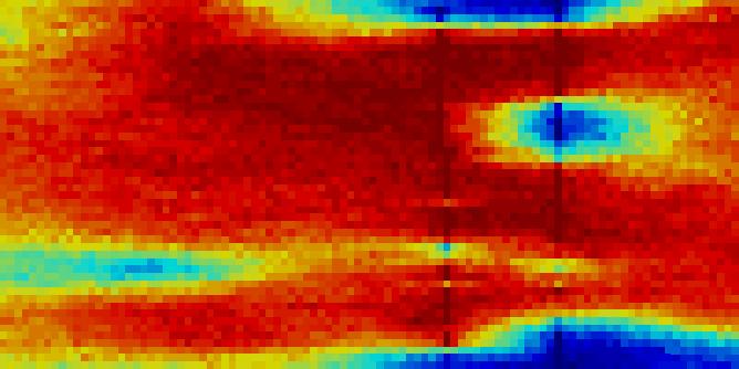
28 Well A Well A (a) Hard data (b) Cosnesim Well B Well C Well A Well A (c) Cosnesim vertical (d) Independent Figure 24: E-type comparison of sisim with range 50 Slice at Z=27 28

29 6.1 Effect on near-by wells Two near by wells (Well B and C) are selected to compare the reservoir model e-type effect on near-by wells. The well locations of Well B and Well C are shown in Figure 24(d). In this case we only compare the proposed algorithm with the normal template (cosnesim), however an additional case is simulated with larger measurement error (ME). Well C was logged in 1978 with older technology compared to Well B, which was logged in From a technology point of view, the newer technology is more reliable than old technology, hence in the case of cosnesim with high ME an arbitrary value of +/- 27.9% in the measurement error was assigned to Well C when computing the data pre-posterior. In the other hand Well B used +/- 7.1% ME. The data pre-posterior of the wells is presented in Figures 25(a) and 25(b). (a) Well B (b) Well C Figure 25: Data pre-posterior, P (A well log) with +/- 5% and high ME compared to hard data Figures 26(a), 27(a) and 28(a) corresponds to the case where hard data is considered for reservoir. Figures 26(b), 27(b) and 28(b) corresponds to the proposed algorithm with error measurement of +/- 5% as in the previous cases. Figures 26(c), 27(c) and 28(c) corresponds to a high error measurement (ME) (especially in Well C) due to the technology used. Figures 26(d), 27(d) and 28(d) corresponds to the independent selection of P (A well log) without considering geological continuity. In the case of a horizontal range of 10, the hard data e-type in Figure 26(a) shows that sand / shale breaks appear in Wells B and C, see circle. In the cosnesim Figure 26(b), the shale breaks are replaced by sand since the geological continuity in the vertical direction has a range of 10, therefore, in addition to the data pre-posterior, the cosnesim algorithm considers the geological continuity of the reservoir model. In the case of large ME in Well C, especially in the sections of logs that are not reliable, the e-type in Figures 26(b) and 26(c) (in a square), shows that with the same geological continuity considered, the data of a more reliable well affects the posterior probability of grid cells near less reliable wells. The independently drawn case shown follows a 29

30 random draw of sand and shale but does not takes the geological continuity into consideration. The same effect can be observed in the cases of range 30 and 50, however the effect in the unreliable sections of Well C when large ME is used (in a square) as shown in Figures 27(b) and 27(c), and Figures 28(b) and 28(c) is less noticeable when the range exceeds 30 because not only Well B affects C but also the reminder 13 wells not considered in this section. Well B Well C Less shale breaks due to vertical range in circle (a) Hard data More reliable Well B makes Well C show more sand in the rectangle (c) Cosnesim high ME (b) Cosnesim In near well cells independent draw does not change posterior probability when range changes (see Fig. 27(d) and 28(d)) (d) Independent Figure 26: E-type comparison of sisim with range 10 Slice at X=28 30

31 Well B Well C Less shale breaks due to vertical range in circle (a) Hard data More reliable Well B makes Well C show more sand in the rectangle (c) Cosnesim high ME (b) Cosnesim In near well cells independent draw does not change posterior probability when range changes (see Fig. 26(d) and 28(d)) (d) Independent Figure 27: E-type comparison of sisim with range 30 Slice at X=28 Well B Well C Less shale breaks due to vertical range in circle (a) Hard data More reliable Well B makes Well C show more sand in the rectangle (c) Cosnesim high ME (b) Cosnesim In near well cells independent draw does not change posterior probability when range changes (see Fig. 26(d) and 27(d)) (d) Independent Figure 28: E-type comparison of sisim with range 50 Slice at X=28 31

32 7 Conclusions A method for uncertainty related to hard data was implemented using 3D real well data. The method does not require the usual assumptions of co-location, Gaussianity or independence, nor does it call for tedious cross-variogram. Instead, an iterative process (cosnesim and cosnesim vertical) are proposed that honors not only the uncertain data but also the spatial geological continuity model provided through a variogram model. The method proposed may overcome the difficulty of integrating sources of different reliability by means of a data pre-posterior instead of constraining the model with hard data. Providing uncertainty on hard data is often very useful when performing history matching. Freezing data at wells may render a history match infeasible in real field cases (Hoffman (2005)). The method generates several realizations of hard data sets which can be used in a further integrated uncertainty analysis by considering other sources of uncertainties. References Akamine, J. and Caers, J.: 2006, Conditioning stochastic realizations to hard data with varying reliability, Report 19, Stanford Center for Reservoir Forecasting, Stanford, CA. Bassiouni, Z.: 1994, Theory, Measurement, and Interpretation of Well Logs, SPE Textbook Series Vol. 4, Society of Petroleum Engineers, Richardson, TX. Hoffman, T.: 2005, History matching while perturbing facies, PhD thesis, Stanford University, Stanford, CA. Journel, A.: 2002, Combining knowledge from diverse sources: An alternative to traditional data independence hypotheses, Mathematical Geology 34(5), Strebelle, S.: 2002, Conditional simulation of complex geological structures using multiple-point statistics, Mathematical Geology 34(1),