CS 558: Computer Vision 4 th Set of Notes

Transcription

1 1 CS 558: Computer Vision 4 th Set of Notes Instructor: Philippos Mordohai Webpage: Philippos.Mordohai@stevens.edu Office: Lieb 215

2 Overview Keypoint matching Hessian detector Blob detection Feature descriptors Fitting RANSAC Based on slides by S. Lazebnik and D. Hoiem 2

3 Overview of Keypoint Matching 1. Find a set of distinctive keypoints A 2 A 1 A3 2. Define a region around each keypoint f A d( f A, f B ) T K. Grauman, B. Leibe f B 3. Extract and normalize the region content 4. Compute a local descriptor from the normalized region 5. Match local descriptors

4 Goals for Keypoints Detect points that are repeatable and distinctive

5 Key trade-offs A 1 A 2 A 3 Detection More Repeatable Robust detection Precise localization More Points Robust to occlusion Works with less texture Description More Distinctive Minimize wrong matches More Flexible Robust to expected variations Maximize correct matches

6 Hessian Detector [Beaudet78] Hessian determinant I xx Hessian ( I) I I xx xy I I xy yy I yy I xy Intuition: Search for strong curvature in two orthogonal directions K. Grauman, B. Leibe

7 Hessian Detector [Beaudet78] Hessian determinant I xx Hessian ( x, ) I I xx xy ( x, ) ( x, ) I I xy yy ( x, ) ( x, ) I yy det M trace M I xy Find maxima of determinant det( Hessian( x)) I xx ( x) I yy ( x) I 2 xy ( x) In Matlab: I xx. I yy ( I xy )^2 K. Grauman, B. Leibe

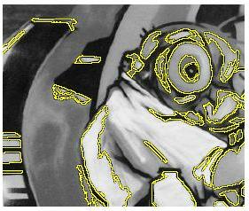
8 Hessian Detector Responses [Beaudet78] Effect: Responses mainly on corners and strongly textured areas.

9 Hessian Detector Responses [Beaudet78]

10 So far: can localize in x-y, but not scale

11 Automatic Scale Selection f I (, )) ( (, i x f I x )) 1im i im ( 1 How to find corresponding patch sizes? K. Grauman, B. Leibe

12 Automatic Scale Selection Function responses for increasing scale (scale signature) ( x, )) f ( I i i m 1 ( x, )) m K. Grauman, B. Leibe i i f ( I 1

13 Automatic Scale Selection Function responses for increasing scale (scale signature) ( x, )) f ( I i i m 1 ( x, )) m K. Grauman, B. Leibe i i f ( I 1

14 Automatic Scale Selection Function responses for increasing scale (scale signature) ( x, )) f I (, )) i i m m K. Grauman, B. Leibe i i f ( I 1 ( 1 x

15 Blob detection

16 Feature detection with scale selection We want to extract features with characteristic scale that is covariant with the image transformation

17 Blob detection: Basic idea To detect blobs, convolve the image with a blob filter at multiple scales and look for extrema of filter response in the resulting scale space

18 Blob detection: Basic idea minima * = maxima Find maxima and minima of blob filter response in space and scale Source: N. Snavely

19 Blob filter Laplacian of Gaussian: Circularly symmetric operator for blob detection in 2D 2 g 2 x g 2 2 y g 2

20 Recall: Edge detection f Edge d dx g Derivative of Gaussian f d dx g Edge = maximum of derivative Source: S. Seitz

21 Edge detection, Take 2 f Edge d dx 2 2 g Second derivative of Gaussian (Laplacian) d dx 2 f 2 g Edge = zero crossing of second derivative Source: S. Seitz

22 From edges to blobs Edge = ripple Blob = superposition of two ripples maximum Spatial selection: the magnitude of the Laplacian response will achieve a maximum at the center of the blob, provided the scale of the Laplacian is matched to the scale of the blob

23 Scale selection We want to find the characteristic scale of the blob by convolving it with Laplacians at several scales and looking for the maximum response However, Laplacian response decays as scale increases: original signal (radius=8) increasing σ

24 Scale normalization The response of a derivative of Gaussian filter to a perfect step edge decreases as σ increases 1 2

25 Scale normalization The response of a derivative of Gaussian filter to a perfect step edge decreases as σ increases To keep response the same (scaleinvariant), must multiply Gaussian derivative by σ Laplacian is the second Gaussian derivative, so it must be multiplied by σ 2

26 Effect of scale normalization Original signal Unnormalized Laplacian response Scale-normalized Laplacian response maximum

27 Blob detection in 2D Laplacian of Gaussian: Circularly symmetric operator for blob detection in 2D Scale-normalized: g g 2 g 2 norm x 2 y 2 2 2

28 Scale selection At what scale does the Laplacian achieve a maximum response to a binary circle of radius r? To get maximum response, the zeros of the Laplacian have to be aligned with the circle The Laplacian is given by (up to scale): ( x 2 y ) ( x Therefore, the maximum response occurs at e 2 y 2 )/ 2 2 r / 2. circle r 0 Laplacian image

29 Characteristic scale We define the characteristic scale of a blob as the scale that produces peak of Laplacian response in the blob center characteristic scale T. Lindeberg (1998). "Feature detection with automatic scale selection." International Journal of Computer Vision 30 (2): pp

30 Scale-space blob detector 1. Convolve image with scale-normalized Laplacian at several scales

31 Scale-space blob detector: Example

32 Scale-space blob detector: Example

33 Scale-space blob detector 1. Convolve image with scale-normalized Laplacian at several scales 2. Find maxima of squared Laplacian response in scale-space

34 Scale-space blob detector: Example

35 Approximating the Laplacian with a difference of Gaussians: 2 L Gxx x y Gyy x y (,, ) (,, ) (Laplacian) Efficient implementation DoG G( x, y, k ) G( x, y, ) (Difference of Gaussians)

36 Efficient implementation David G. Lowe. "Distinctive image features from scale-invariant keypoints. IJCV 60 (2), pp , 2004.

37 Maximally Stable Extremal Regions [Matas 02] Based on Watershed segmentation algorithm Select regions that stay stable over a large parameter range K. Grauman, B. Leibe

38 Example Results: MSER K. Grauman, B. Leibe

39 Local Descriptors The ideal descriptor should be Robust Distinctive Compact Efficient Most available descriptors focus on edge/gradient information Capture texture information Color rarely used K. Grauman, B. Leibe

40 From feature detection to feature description Scaled and rotated versions of the same neighborhood will give rise to blobs that are related by the same transformation What to do if we want to compare the appearance of these image regions? Normalization: transform these regions into same-size circles Problem: rotational ambiguity

41 Eliminating rotation ambiguity To assign a unique orientation to circular image windows: Create histogram of local gradient directions in the patch Assign canonical orientation at peak of smoothed histogram 0 2

42 SIFT features Detected features with characteristic scales and orientations: David G. Lowe. "Distinctive image features from scale-invariant keypoints. IJCV 60 (2), pp , 2004.

43 From feature detection to feature description Detection is covariant: features(transform(image)) = transform(features(image)) Description is invariant: features(transform(image)) = features(image)

44 Properties of SIFT Extraordinarily robust detection and description technique Can handle changes in viewpoint Up to about 60 degree out-of-plane rotation Can handle significant changes in illumination Sometimes even day vs. night Fast and efficient can run in real time Lots of code available Source: N. Snavely

45 Local Descriptors: SIFT Descriptor [Lowe, ICCV 1999] K. Grauman, B. Leibe Histogram of oriented gradients Captures important texture information Robust to small translations / affine deformations

46 Details of Lowe s SIFT algorithm Run DoG detector Find maxima in location/scale space Remove edge points (bad localization) Find all major orientations Bin orientations into 36 bin histogram Weight by gradient magnitude Weight by distance to center (Gaussian-weighted mean) Return orientations within 0.8 of peak of histogram Use parabola for better orientation fit For each (x,y,scale,orientation), create descriptor: Sample 16x16 gradient mag. and rel. orientation Bin 4x4 samples into 4x4 histograms Threshold values to max of 0.2, divide by L2 norm Final descriptor: 4x4x8 normalized histograms r: eigenvalue ratio Lowe IJCV 2004

47 Matching SIFT Descriptors Nearest neighbor (Euclidean distance) Threshold ratio of nearest to 2 nd nearest descriptor Lowe IJCV 2004

48 SIFT Repeatability

49 SIFT Repeatability Lowe IJCV 2004

50 Local Descriptors: SURF Fast approximation of SIFT idea Efficient computation by 2D box filters & integral images 6 times faster than SIFT Equivalent quality for object identification [Bay, ECCV 06], [Cornelis, CVGPU 08] K. Grauman, B. Leibe

51 Local Descriptors: Shape Context Count the number of points inside each bin, e.g.: Count = 4... Count = 10 Log-polar binning: more precision for nearby points, more flexibility for farther points. Belongie & Malik, ICCV 2001 K. Grauman, B. Leibe

52 Choosing a detector What do you want it for? Precise localization in x-y: Harris Good localization in scale: Difference of Gaussian Flexible region shape: MSER Best choice often application dependent Harris-/Hessian-Laplace/DoG work well for many natural categories MSER works well for buildings and printed things Why choose? Get more points with more detectors There have been extensive evaluations/comparisons All detectors/descriptors shown here work well

53 Choosing a descriptor Again, need not stick to one For object instance recognition or stitching, SIFT or variant is a good choice

54 Things to remember Keypoint detection: repeatable and distinctive Corners, blobs, stable regions Harris, DoG Descriptors: robust and selective spatial histograms of orientation SIFT

55 Fitting

56 Fitting We ve learned how to detect edges, corners, blobs. Now what? We would like to form a higher-level, more compact representation of the features in the image by grouping multiple features according to a simple model

57 Fitting Choose a parametric model to represent a set of features simple model: lines simple model: circles complicated model: car Source: K. Grauman

58 Fitting: Overview If we know which points belong to the line, how do we find the optimal line parameters? Least squares What if there are outliers? Robust fitting, RANSAC What if there are many lines? Voting methods: RANSAC, Hough transform What if we re not even sure it s a line? Model selection (not covered)

59 Least squares line fitting Data: (x 1, y 1 ),, (x n, y n ) Line equation: y i = m x i + b Find (m, b) to minimize Y X XB X db de T T b m B x x X y y Y XB Y E n n 1 1 where Pseudo-inverse solution n i i i b mx y E 1 2 ) ( (x i, y i ) y=mx+b Y X XB X T T ) ( ) ( ) 2( ) ( ) ( 2 XB XB Y XB Y Y XB Y XB Y XB Y E T T T T Y X X X B T T 1 ) (

60 Problem with vertical least squares Not rotation-invariant Fails completely for vertical lines

61 Total least squares Distance between point (x i, y i ) and line ax+by=d (a 2 +b 2 =1): ax i + by i d E n i 1 2 ( axi(x b i y, i y d i ) ax+by=d Unit normal: N=(a, b)

62 Total least squares Distance between point (x i, y i ) and line ax+by=d (a 2 +b 2 =1): ax i + by i d Find (a, b, d) to minimize the sum of squared perpendicular distances n E ax b y E n i 1 ( ax i b y i d 2 ) 2 ( i i(x i d 1 i, y i ) ax+by=d Unit normal: N=(a, b)

63 Total least squares Distance between point (x i, y i ) and line ax+by=d (a 2 +b 2 =1): ax i + by i d Find (a, b, d) to minimize the sum of squared perpendicular distances n i i i d b y ax E 1 2 ) ( (x i, y i ) ax+by=d n i i i d b y ax E 1 2 ) ( Unit normal: N=(a, b) 0 ) 2( 1 n i i i d b y ax d E b y ax y n b x n a d n i i n i i 1 1 ) ( ) ( )) ( ) ( ( UN UN b a y y x x y y x x y y b x x a E T n n n i i i 0 ) ( 2 N U U dn de T Solution to (U T U)N = 0, subject to N 2 = 1: eigenvector of U T U associated with the smallest eigenvalue (least squares solution to homogeneous linear system UN = 0)

64 Total least squares y y x x y y x x U n n 1 1 n i i n i i i n i i i n i i T y y y y x x y y x x x x U U ) ( ) )( ( ) )( ( ) ( ), ( y x N = (a, b) second moment matrix ), ( y y x x i i F&P (2 nd ed.) sec. 22.1

65 Least squares: Robustness to noise

66 Least squares: Robustness to noise Problem: squared error heavily penalizes outliers

67 RANSAC Random sample consensus (RANSAC): Very general framework for model fitting in the presence of outliers Outline Choose a small subset of points uniformly at random Fit a model to that subset Find all remaining points that are close to the model and reject the rest as outliers Do this many times and choose the best model M. A. Fischler, R. C. Bolles. Random Sample Consensus: A Paradigm for Model Fitting with Applications to Image Analysis and Automated Cartography. Comm. of the ACM, Vol 24, pp , 1981.

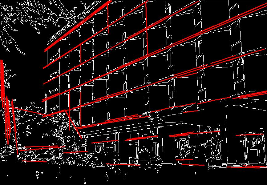
68 RANSAC for line fitting example Source: R. Raguram

69 RANSAC for line fitting example Least squares fit Source: R. Raguram

70 RANSAC for line fitting example 1. Randomly select minimal subset of points Source: R. Raguram

71 RANSAC for line fitting example 1. Randomly select minimal subset of points 2. Hypothesize a model Source: R. Raguram

72 RANSAC for line fitting example 1. Randomly select minimal subset of points 2. Hypothesize a model 3. Compute error function Source: R. Raguram

73 RANSAC for line fitting example 1. Randomly select minimal subset of points 2. Hypothesize a model 3. Compute error function 4. Select points consistent with model Source: R. Raguram

74 RANSAC for line fitting example 1. Randomly select minimal subset of points 2. Hypothesize a model 3. Compute error function 4. Select points consistent with model 5. Repeat hypothesize andverify loop Source: R. Raguram

75 RANSAC for line fitting example 1. Randomly select minimal subset of points 2. Hypothesize a model 3. Compute error function 4. Select points consistent with model 5. Repeat hypothesize andverify loop Source: R. Raguram

76 RANSAC for line fitting example Uncontaminated sample 1. Randomly select minimal subset of points 2. Hypothesize a model 3. Compute error function 4. Select points consistent with model 5. Repeat hypothesize andverify loop Source: R. Raguram

77 RANSAC for line fitting example 1. Randomly select minimal subset of points 2. Hypothesize a model 3. Compute error function 4. Select points consistent with model 5. Repeat hypothesize andverify loop Source: R. Raguram

78 RANSAC for line fitting Repeat N times: Draw s points uniformly at random Fit line to these s points Find inliers to this line among the remaining points (i.e., points whose distance from the line is less than t) If there are d or more inliers, accept the line and refit using all inliers

79 Choosing the parameters Initial number of points s Typically minimum number needed to fit the model Distance threshold t Choose t so probability for inlier is p (e.g. 0.95) Zero-mean Gaussian noise with std. dev. σ: t 2 =3.84σ 2 Number of samples N Choose N so that, with probability p, at least one random sample is free from outliers (e.g. p=0.99) (outlier ratio: e) Source: M. Pollefeys

80 Choosing the parameters Initial number of points s Typically minimum number needed to fit the model Number of samples N Choose N so that, with probability p, at least one random sample is free from outliers (e.g. p=0.99) (outlier ratio: e) s N 1 1 e 1 p N p/ log1 e log 1 1 s proportion of outliers e s 5% 10% 20% 25% 30% 40% 50% Source: M. Pollefeys

81 Choosing the parameters Initial number of points s Typically minimum number needed to fit the model Distance threshold t Choose t so probability for inlier is p (e.g. 0.95) Zero-mean Gaussian noise with std. dev. σ: t 2 =3.84σ 2 Number of samples N Choose N so that, with probability p, at least one random sample is free from outliers (e.g. p=0.99) (outlier ratio: e) Consensus set size d Should match expected inlier ratio Source: M. Pollefeys

82 Adaptively determining the number of samples Outlier ratio e is often unknown a priori, so pick worst case, e.g. 50%, and adapt if more inliers are found, e.g. 80% would yield e=0.2 Adaptive procedure: N=, sample_count =0 While N >sample_count Choose a sample and count the number of inliers If inlier ratio is highest of any found so far, set e = 1 (number of inliers)/(total number of points) Recompute N from e: N p/ log1 e log 1 1 Increment the sample_count by 1 s Source: M. Pollefeys

83 RANSAC pros and cons Pros Simple and general Applicable to many different problems Often works well in practice Cons Computational time grows quickly with fraction of outliers and number of parameters Not as good for getting multiple fits (though one solution is to remove inliers after each fit and repeat) Sensitivity to threshold t

84 Slide Credits This set of sides contains contributions kindly made available by the following authors Derek Hoiem Svetlana Lazebnik Kristen Grauman Bastian Leibe David Lowe Marc Pollefeys Rahul Raguram Steve Seitz Noah Snavely