Chapter 5: Introduction to Differential Analysis of Fluid Motion

Transcription

1 Chapter 5: Introduction to Differential 5-1 Conservation of Mass 5-2 Stream Function for Two-Dimensional 5-3 Incompressible Flow 5-4 Motion of a Fluid Particle (Kinematics) 5-5 Momentum Equation 5-6 Computational Fluid Dynamics (CFD) 5-7 Exact Solutions of the Navier-Stokes Equation Chapter 5 Introduction to Differential

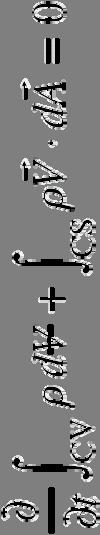
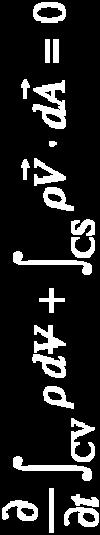
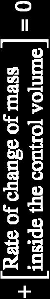
2 5-1 Conservation of Mass (1) Basic Law for a System: 5-1

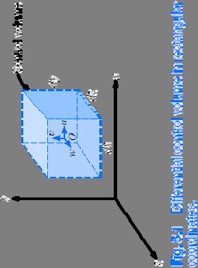
3 5-1 Conservation of Mass (2) Rectangular Coordinate System: 5-2

4 5-1 Conservation of Mass (3) Rectangular Coordinate System: Continuity Equation Ignore terms higher than order dx 5-3

5 5-1 Conservation of Mass (4) Rectangular Coordinate System: Del Operator 5-4

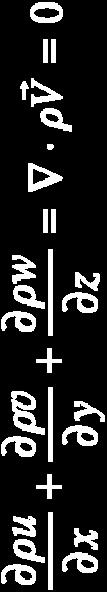
6 5-1 Conservation of Mass (5) Rectangular Coordinate System: Incompressible Fluid: Steady Flow: 5-5

7 5-1 Conservation of Mass (6) Cylindrical Coordinate System: 5-6

8 5-1 Conservation of Mass (7) Cylindrical Coordinate System: Del Operator 5-7

9 5-1 Conservation of Mass (8) Cylindrical Coordinate System: Incompressible Fluid: Steady Flow: 5-8

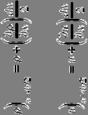
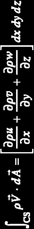
10 5-1 Conservation of Mass (9) Alternative Method: Divergence Theorem: Divergence theorem allows us to transform a volume integral of the divergence of a vector into an area integral over the surface that defines the volume. 5-9

11 5-1 Conservation of Mass (10) Rewrite conservation of momentum Using divergence theorem, replace area integral with volume integral and collect terms Integral holds for ANY CV, therefore: 5-10

12 5-1 Conservation of Mass (11) Alternative form: 5-11

13 5-2 Stream Function for Two-Dimensional Incompressible Flow (1) Two-Dimensional Flow: Stream Function ψ This is true for any smooth function ψ(x,y) 5-12

14 5-2 Stream Function for Two-Dimensional Incompressible Flow (2) Why do this? Single variable ψ replaces (u,v). Once ψ is known, (u,v) can be computed. Physical significance Curves of constant ψ are streamlines of the flow Difference in ψ between streamlines is equal to volume flow rate between streamlines 5-13

15 5-2 Stream Function for Two-Dimensional Incompressible Flow (3) Physical Significance: Recall that along astreamline Change in ψ along streamline is zero 5-14

16 5-2 Stream Function for Two-Dimensional Incompressible Flow (4) Physical Significance: Difference in ψ between streamlines is equal to volume flow rate between streamlines 5-15

17 5-2 Stream Function for Two-Dimensional Incompressible Flow (5) Cylindrical Coordinates: Stream Function ψ(r,θ) 5-16

18 5-3 Motion of a Fluid Particle (Kinematics) (1) Lagrangian Description: Lagrangian description of fluid flow tracks the position and velocity of individual particles. Based upon Newton's laws of motion. Difficult to use for practical flow analysis. Fluids are composed of billions of molecules. Interaction between molecules hard to describe/model. However, useful for specialized applications Sprays, particles, bubble dynamics, rarefied gases. Coupled Eulerian-Lagrangian methods. Named after Italian mathematician Joseph Louis Lagrange ( ). 5-17

19 5-3 Motion of a Fluid Particle (Kinematics) (2) Eulerian Description: Eulerian description of fluid flow: a flow domain or control volume is defined by which fluid flows in and out. We define field variables which are functions of space and time. Pressure field, P=P(x,y,z,t) r r Velocity field, V r r r r V= uxyzti+ vxyzt j+ wxyztk Acceleration field, = V( x, y, z, t) (,,, ) (,,, ) (,,, ) r r a = a x y z t (,,, ) r r r r a= a xyzti+ a xyzt j+ a xyztk (,,, ) (,,, ) (,,, ) x y z These (and other) field variables define the flow field. Well suited for formulation of initial boundary-value problems (PDE's). Named after Swiss mathematician Leonhard Euler ( ). 5-18

20 5-3 Motion of a Fluid Particle (Kinematics) (3) Fluid Translation: Acceleration of a Fluid Particle in a Velocity Field Fluid Rotation Fluid Deformation Angular Deformation Linear Deformation 5-19

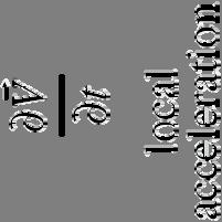
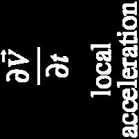
21 5-3 Motion of a Fluid Particle (Kinematics) (4) Acceleration Field Consider a fluid particle and Newton's second law, r r F = m a particle particle particle The acceleration of the particle is the time derivative of the particle's velocity. r r a particle = particle However, particle velocity at a point is the same as the fluid r r velocity, Vparticle = V( xparticle ( t), yparticle ( t), zparticle ( t) ) To take the time derivative of, chain rule must be used. r a particle dv r r r r Vdt Vdx Vdy Vdz = t dt x dt y dt z dt dt particle particle particle 5-20

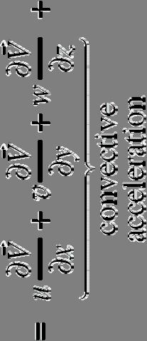
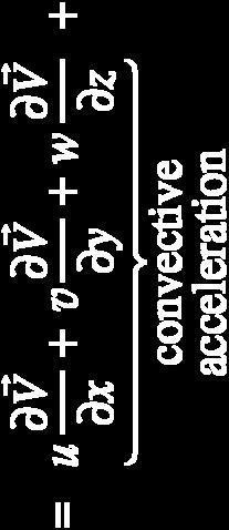
22 5-3 Motion of a Fluid Particle (Kinematics) (5) Since dxparticle dy particle dz particle = u, = v, = w dt dt dt In vector form, the acceleration can be written as r r r r r V V V V aparticle = + u + v + w t x y z 5-21

23 5-3 Motion of a Fluid Particle (Kinematics) (6) Fluid Translation: Acceleration of a Fluid Particle in a Velocity Field: 5-22

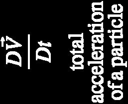
24 5-3 Motion of a Fluid Particle (Kinematics) (7) The total derivative operator d/dt is call the material derivative and is often given special notation, D/Dt. Advective acceleration is nonlinear: source of many phenomenon and primary challenge in solving fluid flow problems. Provides ``transformation'' between Lagrangian and Eulerian frames. Other names for the material derivative include: total, particle, Lagrangian, Eulerian, and substantial derivative. 5-23

25 5-3 Motion of a Fluid Particle (Kinematics) (8) There is a direct analogy between the transformation from Lagrangian to Eulerian descriptions (for differential analysis using infinitesimally small fluid elements) and the transformation from systems to control volumes (for integral analysis using large, finite flow fields). 5-24

26 5-3 Motion of a Fluid Particle (Kinematics) (9) Flow Visualization: Flow visualization is the visual examination of flowfield features. Important for both physical experiments and numerical (CFD) solutions. Numerous methods Streamlines and streamtubes Pathlines Streaklines Timelines Refractive techniques Surface flow techniques 5-25

27 5-3 Motion of a Fluid Particle (Kinematics) (10) Streamlines A Streamline is a curve that is everywhere tangent to the instantaneous local velocity vector. Consider an arc length r r r r dr = dxi + dyj + dzk dr r must be parallel to the local velocity V r = ui r vector + vj r + wk r Geometric arguments results in the equation for a streamline dr dx dy dz = = = V u v w 5-26

28 5-3 Motion of a Fluid Particle (Kinematics) (11) Streamlines NASCAR surface pressure contours and streamlines Airplane surface pressure contours, volume streamlines, and surface streamlines 5-27

29 5-3 Motion of a Fluid Particle (Kinematics) (12) Pathline A Pathline is the actual path traveled by an individual fluid particle over some time period. Same as the fluid particle's material position vector ( xparticle ( t), yparticle ( t), zparticle ( t) ) Particle location at time t: t r = start + r t r x x Vdt start Particle Image Velocimetry (PIV) is a modern experimental technique to measure velocity field over a plane in the flow field. 5-28

30 5-3 Motion of a Fluid Particle (Kinematics) (13) Streakline: A Streakline is the locus of fluid particles that have passed sequentially through a prescribed point in the flow. Easy to generate in experiments: dye in a water flow, or smoke in an airflow. 5-29

31 5-3 Motion of a Fluid Particle (Kinematics) (14) For steady flow, streamlines, pathlines, and streaklines are identical. For unsteady flow, they can be very different. Streamlines are an instantaneous picture of the flow field Pathlines and Streaklines are flow patterns that have a time history associated with them. Streakline: instantaneous snapshot of a timeintegrated flow pattern. Pathline: time-exposed flow path of an individual particle. 5-30

32 5-3 Motion of a Fluid Particle (Kinematics) (15) In fluid mechanics, an element may undergo four fundamental types of motion. a) Translation b) Rotation c) Linear strain d) Shear strain Because fluids are in constant motion, motion and deformation is best described in terms of rates a) velocity: rate of translation b) angular velocity: rate of rotation c) linear strain rate: rate of linear strain d) shear strain rate: rate of shear strain 5-31

33 5-3 Motion of a Fluid Particle (Kinematics) (16) Fluid Translation: Acceleration of a Fluid Particle in a Velocity Field: 5-32

34 5-4 Motion of a Fluid Particle (Kinematics) (17) Fluid Translation: Acceleration of a Fluid Particle in a Velocity Field (Cylindrical): 5-33

35 5-4 Motion of a Fluid Particle (Kinematics) (18) Fluid Rotation: 5-34

36 5-4 Motion of a Fluid Particle (Kinematics) (19) Vorticity and Rotationality: The vorticity vector is defined as the curl of the r r r velocity vector ζ = V Vorticity is equal to twice the angular velocity of a fluid particle. r r Cartesian coordinates ζ = 2ω r w v r u w r v u r ζ = i + j + k y z z x x y Cylindrical coordinates In regions where z = 0, the flow is called irrotational. Elsewhere, the flow is called rotational. ( ru ) r 1 uz uθ r ur uz r θ u r r ζ = er + eθ + e r θ z z r r θ z 5-35

37 5-4 Motion of a Fluid Particle (Kinematics) (20) Vorticity and Rotationality: 5-36

38 5-4 Motion of a Fluid Particle (Kinematics) (21) Comparison of Two Circular Flows: Special case: consider two flows with circular streamlines ur = 0, uθ = ωr 2 r 1 ( ru ) u 1 ( r θ ) r r ω r r ζ = e = 0 e = 2ωe r r θ r r z z z K ur = 0, uθ = r r 1 ( ruθ ) u r r 1 ( K ) r r ζ = e = 0 e = 0e r r θ r r z z z 5-37

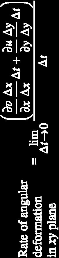
39 5-4 Motion of a Fluid Particle (Kinematics) (22) Fluid Deformation: Angular Deformation 5-38

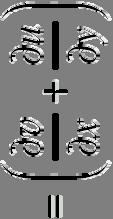
40 5-4 Motion of a Fluid Particle (Kinematics) (23) Shear Strain Rate at a point is defined as half of the rate of decrease of the angle between two initially perpendicular lines that intersect at a point. Shear strain rate can be expressed in Cartesian coordinates as: 1 u v 1 1 xy, w u zx, v ε ε ε w = yz 2 + = + = + y x 2 x z 2 z y 5-39

41 5-4 Motion of a Fluid Particle (Kinematics) (24) We can combine linear strain rate and shear strain rate into one symmetric second-order tensor called the strain-rate tensor. u 1 u v 1 u w + + x 2 y x 2 z x εxx εxy ε xz 1 v u v 1 v w εij = εyx εyy εyz = 2 + x y y 2 + z y εzx εzy ε zz 1 w u 1 w v w x z 2 y z z 5-40

42 5-4 Motion of a Fluid Particle (Kinematics) (25) Fluid Deformation: Linear Deformation 5-41

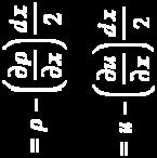
43 5-4 Motion of a Fluid Particle (Kinematics) (26) Linear Strain Rate is defined as the rate of increase in length per unit length. In Cartesian coordinates u xx, v ε = εyy =, ε w zz = x y z Volumetric strain rate in Cartesian coordinates 1 DV u v = ε w xx + εyy + εzz = + + V Dt x y z Since the volume of a fluid element is constant for an incompressible flow, the volumetric strain rate must be zero. 5-42

44 5-5 Momentum Equation (1) Newton s Second Law: 5-43

45 5-5 Momentum Equation (2) Forces Acting on a Fluid Particle: 5-44

46 5-5 Momentum Equation (3) Differential Momentum Equation: or 5-45

47 5-5 Momentum Equation (4) Stress Tensor: σ xx σ xy σ xz p 0 0 τ xx τ xy τ xz σ ij = σ yx σ yy σ yz = 0 p 0 σ zx σ zy σ + τ yx τ yy τ yz zz 0 0 p τ zx τ zy τ zz Viscous (Deviatoric) Stress Tensor 5-46

48 5-5 Momentum Equation (5) Unfortunately, this equation is not very useful 10 unknowns Stress tensor, σ ij : 6 independent components Density ρ Velocity, V : 3 independent components 4 equations (continuity + momentum) 6 more equations required to close problem! 5-47

49 5-5 Momentum Equation (6) First step is to separate σ ij into pressure and viscous stresses σ xx σ xy σ xz p 0 0 τ xx τ xy τ xz σ ij = σ yx σ yy σ yz = 0 p 0 σ zx σ zy σ + τ yx τ yy τ yz zz 0 0 p τ zx τ zy τ zz Situation not yet improved Viscous (Deviatoric) Stress Tensor 6 unknowns in σ ij 6 unknowns in τ ij + 1 in P, which means that we ve added 1! 5-48

50 5-5 Momentum Equation (7) Reduction in the number of variables is achieved by relating shear stress to strainrate tensor. For Newtonian fluid with constant properties Newtonian fluid includes most common fluids: air, other gases, water, gasoline Newtonian closure is analogous to Hooke s Law for elastic solids 5-49

51 5-5 Momentum Equation (8) Substituting Newtonian closure into stress tensor gives Using the definition of ε ij 5-50

52 5-5 Momentum Equation (9) Substituting σ ij into Cauchy s equation gives the Navier-Stokes equations Incompressible NSE written in vector form This results in a closed system of equations! 4 equations (continuity and momentum equations) 4 unknowns (U, V, W, p) 5-51

53 5-5 Momentum Equation (10) Navier-Stokes Equation: In addition to vector form, incompressible N-S equation can be written in several other forms Cartesian coordinates Cylindrical coordinates Tensor notation 5-52

54 5-5 Momentum Equation (11) Newtonian Fluid: Navier-Stokes Equations: 5-53

55 5-5 Momentum Equation (12) Tensor and Vector notation offer a more compact form of the equations. Continuity Tensor notation Vector notation Tensor notation Conservation of Momentum Vector notation Repeated indices are summed over j (x 1 = x, x 2 = y, x 3 = z, U 1 = U, U 2 = V, U 3 = W) 5-54

56 5-5 Momentum Equation (13) Special Case: Euler s Equation 5-55

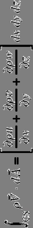
57 5-5 Momentum Equation (14) Alternative method: Body Force Surface Force σ ij = stress tensor Using the divergence theorem to convert area integrals 5-56

58 5-5 Momentum Equation (15) *Recognizing that this holds for any CV, the integral may be dropped This is Cauchy s Equation Can also be derived using infinitesimal CV and Newton s 2nd Law 5-57

59 5-5 Momentum Equation (16) Alternate form of the Cauchy Equation can be derived by introducing Inserting these into Cauchy Equation and rearranging gives 5-58

60 5-6 Computational Fluid Dynamics (1) Some Applications: 5-59

61 5-6 Computational Fluid Dynamics (2) Discretization: 5-60

62 5-7 Exact Solutions of the Navier Stokes Equation (1) Recall Chap 4: Control volume (CV) versions of the laws of conservation of mass and energy Chap 5: CV version of the conservation of momentum CV, or integral, forms of equations are useful for determining overall effects However, we cannot obtain detailed knowledge about the flow field inside the CV motivation for differential analysis 5-61

63 5-7 Exact Solutions of the Navier Stokes Equation (2) Example: incompressible Navier-Stokes equations We will learn: Physical meaning of each term How to derive How to solve 5-62

64 5-7 Exact Solutions of the Navier Stokes Equation (3) For example, how to solve? Step 1 Analytical Fluid Dynamics Setup Problem and geometry, identify all dimensions and parameters List all assumptions, approximations, simplifications, boundary conditions Simplify PDE s Integrate equations Apply I.C. s and B.C. s to solve for constants of integration Verify and plot results 5-63

65 5-7 Exact Solutions of the Navier Stokes Equation (4) Navier-Stokes equations Incompressible NSE written in vector form This results in a closed system of equations! 4 equations (continuity and momentum equations) 4 unknowns (U, V, W, p) 5-64

66 5-7 Exact Solutions of the Navier Stokes Equation (5) Continuity X-momentum Y-momentum Z-momentum 5-65

67 5-7 Exact Solutions of the Navier Stokes Equation (6) There are about 80 known exact solutions to the NSE (Navier- Stokes Equation) The can be classified as: Linear solutions where the convective term is zero Nonlinear solutions where convective term is not zero Solutions can also be classified by type or geometry 1. Couette shear flows 2. Steady duct/pipe flows 3. Unsteady duct/pipe flows 4. Flows with moving boundaries 5. Similarity solutions 6. Asymptotic suction flows 7. Wind-driven Ekman flows 5-66

68 5-7 Exact Solutions of the Navier Stokes Equation (7) No-slip boundary condition: For a fluid in contact with a solid wall, the velocity of the fluid must equal that of the wall 5-67

69 5-7 Exact Solutions of the Navier Stokes Equation (8) Interface boundary condition: When two fluids meet at an interface, the velocity and shear stress must be the same on both sides If surface tension effects are negligible and the surface is nearly flat 5-68

70 5-7 Exact Solutions of the Navier Stokes Equation (9) Interface boundary condition: Degenerate case of the interface BC occurs at the free surface of a liquid. Same conditions hold Since μ air << μ water, As with general interfaces, if surface tension effects are negligible and the surface is nearly flat P water = P air 5-69

71 5-7 Exact Solutions of the Navier Stokes Equation (10) Example exact solution: Fully Developed Couette Flow For the given geometry and BC s, calculate the velocity and pressure fields, and estimate the shear force per unit area acting on the bottom plate Step 1: Geometry, dimensions, and properties 5-70

72 5-7 Exact Solutions of the Navier Stokes Equation (11) Step 2: Assumptions and BC s Assumptions 1. Plates are infinite in x and z 2. Flow is steady, / t = 0 3. Parallel flow, V=0 4. Incompressible, Newtonian, laminar, constant properties 5. No pressure gradient 6. 2D, W=0, / z = 0 7. Gravity acts in the -z direction, Boundary conditions 1. Bottom plate (y=0) : u=0, v=0, w=0 2. Top plate (y=h) : u=v, v=0, w=0 5-71

73 5-7 Exact Solutions of the Navier Stokes Equation (12) Step 3: Simplify Continuity 3 6 Note: these numbers refer to the assumptions on the previous slide X-momentum This means the flow is fully developed or not changing in the direction of flow 2 Cont Cont

74 5-7 Exact Solutions of the Navier Stokes Equation (13) Step 3: Simplify, cont. Y-momentum 2, , Z-momentum 2,

75 5-7 Exact Solutions of the Navier Stokes Equation (14) Step 4: Integrate X-momentum integrate integrate Z-momentum integrate 5-74

76 5-7 Exact Solutions of the Navier Stokes Equation (15) Step 5: Apply BC s y=0, u=0=c 1 (0) + C 2 C 2 = 0 y=h, u=v=c 1 h C 1 = V/h This gives For pressure, no explicit BC, therefore C 3 can remain an arbitrary constant (recall only P appears in NSE). Let p = p 0 at z = 0 (C 3 renamed p 0 ) 1. Hydrostatic pressure 2. Pressure acts independently of flow 5-75

77 5-7 Exact Solutions of the Navier Stokes Equation (16) Step 6: Verify solution by back-substituting into differential equations Given the solution (u,v,w)=(vy/h, 0, 0) Continuity is satisfied = 0 X-momentum is satisfied 5-76

78 5-7 Exact Solutions of the Navier Stokes Equation (17) Finally, calculate shear force on bottom plate Shear force per unit area acting on the wall Note that τ w is equal and opposite to the shear stress acting on the fluid τ yx (Newton s third law). 5-77